SimpleMKL
Alain Rakotomamonjy [email protected]
LITIS EA 4108 Universit´e de Rouen
76800 Saint Etienne du Rouvray, France
Francis R. Bach [email protected]
INRIA - WILLOW Project - Team
Laboratoire d’Informatique de l’Ecole Normale Sup´erieure(CNRS/ENS/INRIA UMR 8548) 45, Rue d’Ulm, 75230 Paris, France
St´ephane Canu [email protected]
LITIS EA 4108 INSA de Rouen
76801 Saint Etienne du Rouvray, France
Yves Grandvalet [email protected]
Idiap Research Institute, Centre du Parc, 1920 Martigny, Switzerland
Heudiasyc, CNRS/Universit´e de Technologie de Compi`egne (UMR 6599), 60205 Compi`egne, France
Editor: Nello Cristianini
Abstract
Multiple kernel learning (MKL) aims at simultaneously learning a kernel and the associ-ated predictor in supervised learning settings. For the support vector machine, an efficient and general multiple kernel learning algorithm, based on semi-infinite linear progamming, has been recently proposed. This approach has opened new perspectives since it makes MKL tractable for large-scale problems, by iteratively using existing support vector ma-chine code. However, it turns out that this iterative algorithm needs numerous iterations for converging towards a reasonable solution. In this paper, we address the MKL prob-lem through a weighted 2-norm regularization formulation with an additional constraint on the weights that encourages sparse kernel combinations. Apart from learning the com-bination, we solve a standard SVM optimization problem, where the kernel is defined as a linear combination of multiple kernels. We propose an algorithm, named SimpleMKL, for solving this MKL problem and provide a new insight on MKL algorithms based on mixed-norm regularization by showing that the two approaches are equivalent. We show how SimpleMKL can be applied beyond binary classification, for problems like regression, clustering (one-class classification) or multiclass classification. Experimental results show that the proposed algorithm converges rapidly and that its efficiency compares favorably to other MKL algorithms. Finally, we illustrate the usefulness of MKL for some regres-sors based on wavelet kernels and on some model selection problems related to multiclass classification problems.
1. Introduction
During the last few years, kernel methods, such as support vector machines (SVM) have proved to be efficient tools for solving learning problems like classification or regression (Sch¨olkopf and Smola, 2001). For such tasks, the performance of the learning algorithm strongly depends on the data representation. In kernel methods, the data representation
is implicitly chosen through the so-called kernel K(x, x0). This kernel actually plays two
roles: it defines the similarity between two examplesxandx0, while defining an appropriate
regularization term for the learning problem. Let{xi, yi}`
i=1be the learning set, wherexi belongs to some input spaceX and yiis the
target value for pattern xi. For kernel algorithms, the solution of the learning problem is
of the form f(x) = ` X i=1 α?iK(x, xi) +b?, (1) whereα?
i and b? are some coefficients to be learned from examples, while K(·,·) is a given
positive definite kernel associated with a reproducing kernel Hilbert space (RKHS)H.
In some situations, a machine learning practitioner may be interested in more flexible models. Recent applications have shown that using multiple kernels instead of a single one can enhance the interpretability of the decision function and improve performances (Lanckriet et al., 2004a). In such cases, a convenient approach is to consider that the kernel
K(x, x0) is actually a convex combination ofbasis kernels:
K(x, x0) = M X m=1 dmKm(x, x0) , withdm ≥0, M X m=1 dm= 1 ,
whereM is the total number of kernels. Each basis kernelKmmay either use the full set of
variables describingx or subsets of variables stemming from different data sources
(Lanck-riet et al., 2004a). Alternatively, the kernels Km can simply be classical kernels (such as
Gaussian kernels) with different parameters. Within this framework, the problem of data
representation through the kernel is then transferred to the choice of weightsdm.
Learning both the coefficientsαi and the weightsdm in a single optimization problem is
known as the multiple kernel learning (MKL) problem. For binary classification, the MKL problem has been introduced by Lanckriet et al. (2004b), resulting in a quadratically con-strained quadratic programming problem that becomes rapidly intractable as the number of learning examples or kernels become large.
What makes this problem difficult is that it is actually a convex but non-smooth min-imization problem. Indeed, Bach et al. (2004a) have shown that the MKL formulation of Lanckriet et al. (2004b) is actually the dual of a SVM problem in which the weight vector
has been regularized according to a mixed (`2, `1)-norm instead of the classical squared
`2-norm. Bach et al. (2004a) have considered a smoothed version of the problem for which
they proposed a SMO-like algorithm that enables to tackle medium-scale problems. Sonnenburg et al. (2006) reformulate the MKL problem of Lanckriet et al. (2004b) as a semi-infinite linear program (SILP). The advantage of the latter formulation is that the algorithm addresses the problem by iteratively solving a classical SVM problem with a single kernel, for which many efficient toolboxes exist (Vishwanathan et al., 2003; Loosli et al.,
2005; Chang and Lin, 2001), and a linear program whose number of constraints increases along with iterations. A very nice feature of this algorithm is that is can be extended to a large class of convex loss functions. For instance, Zien and Ong (2007) have proposed a multiclass MKL algorithm based on similar ideas.
In this paper, we present another formulation of the multiple learning problem. We first depart from the primal formulation proposed by Bach et al. (2004a) and further used by Bach et al. (2004b) and Sonnenburg et al. (2006). Indeed, we replace the mixed-norm
regu-larization by a weighted`2-norm regularization, where the sparsity of the linear combination
of kernels is controlled by a `1-norm constraint on the kernel weights. This new
formula-tion of MKL leads to a smooth and convex optimizaformula-tion problem. By using a variaformula-tional formulation of the mixed-norm regularization, we show that our formulation is equivalent to the ones of Lanckriet et al. (2004b), Bach et al. (2004a) and Sonnenburg et al. (2006).
The main contribution of this paper is to propose an efficient algorithm, named Sim-pleMKL, for solving the MKL problem, through a primal formulation involving a weighted
`2-norm regularization. Indeed, our algorithm is simple, essentially based on a gradient
descent on the SVM objective value. We iteratively determine the combination of kernels by a gradient descent wrapping a standard SVM solver, which is SimpleSVM in our case. Our scheme is similar to the one of Sonnenburg et al. (2006), and both algorithms minimize the same objective function. However, they differ in that we use reduced gradient descent in the primal, whereas Sonnenburg et al.’s SILP relies on cutting planes. We will empirically show that our optimization strategy is more efficient, with new evidences confirming the preliminary results reported in Rakotomamonjy et al. (2007).
Then, extensions of SimpleMKL to other supervised learning problems such as regression SVM, one-class SVM or multiclass SVM problems based on pairwise coupling are proposed. Although it is not the main purpose of the paper, we will also discuss the applicability of our approach to general convex loss functions.
This paper also presents several illustrations of the usefulness of our algorithm. For instance, in addition to the empirical efficiency comparison, we also show, in a SVM regres-sion problem involving wavelet kernels, that automatic learning of the kernels leads to far better performances. Then we depict how our MKL algorithm behaves on some multiclass problems.
The paper is organized as follows. Section 2 presents the functional settings of our MKL problem and its formulation. Details on the algorithm and discussion of convergence and computational complexity are given in Section 3. Extensions of our algorithm to other SVM problems are discussed in Section 4 while experimental results dealing with computa-tional complexity or with comparison with other model selection methods are presented in Section 5.
A SimpleMKL toolbox based on Matlab code is available at http://www.mloss.org.
This toolbox is an extension of our SVM-KM toolbox (Canu et al., 2003). 2. Multiple Kernel Learning Framework
In this section, we present our MKL formulation and derive its dual. In the sequel, i
we omit to specify that summations on iand j go from 1 to`, and that summations onm
go from 1 toM.
2.1 Functional framework
Before entering into the details of the MKL optimization problem, we first present the
functional framework adopted for multiple kernel learning. Assume Km, m = 1, ..., M are
M positive definite kernels on the same input spaceX, each of them being associated with
an RKHSHm endowed with an inner product h·,·im. For anym, letdm be a non-negative
coefficient andH0
m be the Hilbert space derived from Hm as follows:
H0m ={f |f ∈ Hm : kfkHm
dm
<∞} ,
endowed with the inner product
hf, giH0
m =
1
dmhf, gim .
In this paper, we use the convention that x0 = 0 if x = 0 and ∞ otherwise. This means
that, ifdm = 0 then a function f belongs to the Hilbert space H0m only iff = 0∈ Hm. In
such a case, H0
m is restricted to the null element ofHm.
Within this framework,H0
m is a RKHS with kernelK(x, x0) =dm Km(x, x0) since
∀f ∈ H0m ⊆ Hm , f(x) = hf(·), Km(x,·)im
= 1
dmhf(·), dmKm(x,·)im
= hf(·), dmKm(x,·)iH0
m .
Now, if we defineH as the direct sum of the spacesH0
m, i.e., H= M M m=1 H0m ,
then, a classical result on RKHS (Aronszajn, 1950) says thatH is a RKHS of kernel
K(x, x0) =
M
X
m=1
dmKm(x, x0) .
Owing to this simple construction, we have built a RKHSHfor which any function is a
sum of functions belonging toHm. In our framework, MKL aims at determining the set of
coefficients {dm} within the learning process of the decision function. The multiple kernel
learning problem can thus be envisioned as learning a predictor belonging to an adaptive hypothesis space endowed with an adaptive inner product. The forthcoming sections explain how we solve this problem.
2.2 Multiple kernel learning primal problem
In the SVM methodology, the decision function is of the form given in equation (1),
where the optimal parameters α?
i and b? are obtained by solving the dual of the following
optimization problem: min f,b,ξ 1 2kfk 2 H+C X i ξi s.t. yi(f(xi) +b)≥1−ξi ∀i ξi≥0 ∀i .
In the MKL framework, one looks for a decision function of the form f(x) +b =
P
mfm(x) +b, where each function fm belongs to a different RKHS Hm associated with
a kernel Km. According to the above functional framework and inspired by the multiple
smoothing splines framework of Wahba (1990, chap. 10), we propose to address the MKL SVM problem by solving the following convex problem (see proof in appendix), which we will be referred to as the primal MKL problem:
min {fm},b,ξ,d 1 2 X m 1 dm kfmk2Hm+CX i ξi s.t. yi X m fm(xi) +yib≥1−ξi ∀i ξi ≥0 ∀i X m dm= 1 , dm≥0 ∀m , (2)
where eachdm controls the squared norm of fm in the objective function.
The smallerdmis, the smootherfm (as measured bykfmkHm) should be. Whendm = 0,
kfmkHm has also to be equal to zero to yield a finite objective value. The`1-norm constraint
on the vectordis a sparsity constraint that will force somedmto be zero, thus encouraging
sparse basis kernel expansions.
2.3 Connections with mixed-norm regularization formulation of MKL
The MKL formulation introduced by Bach et al. (2004a) and further developed by Son-nenburg et al. (2006) consists in solving an optimization problem expressed in a functional form as min {f},b,ξ 1 2 Ã X m kfmkHm !2 +CX i ξi s.t. yi X m fm(xi) +yib≥1−ξi ∀i ξi≥0 ∀i. (3)
Note that the objective function of this problem is not smooth sincekfmkHm is not
differen-tiable atfm = 0. However, what makes this formulation interesting is that the mixed-norm
penalization off =Pmfm is a soft-thresholding penalizer that leads to a sparse solution,
for which the algorithm performs kernel selection (Bach, 2008). We have stated in the previous section that our problem should also lead to sparse solutions. In the following, we show that the formulations (2) and (3) are equivalent.
For this purpose, we simply show that the variational formulation of the mixed-norm regularization is equal to the weighted 2-norm regularization, (which is a particular case of a more general equivalence proposed by Micchelli and Pontil (2005)) i.e., by Cauchy-Schwartz
inequality, for any vectordon the simplex:
à X m kfmkHm !2 = à X m kfmkHm d1m/2 d1m/2 !2 6 à X m kfmk2Hm dm ! à X m dm ! 6 X m kfmk2Hm dm ,
where equality is met whend1m/2 is proportional to kfmkHm/d1m/2, that is:
dm= XkfmkHm q kfqkHq , (4) which leads to min dm≥0,Pmdm=1 X m kfmk2Hm dm = Ã X m kfmkHm !2 . (5)
Hence, owing to this variational formulation, the non-smooth mixed-norm objective function of problem (3) has been turned into a smooth objective function in problem (2). Although the number of variables has increased, we will see that this problem can be solved more efficiently.
2.4 The MKL dual problem
The dual problem is a key point for deriving MKL algorithms and for studying their convergence properties. Since our primal problem (2) is equivalent to the one of Bach et al. (2004a), they lead to the same dual. However, our primal formulation being convex and differentiable, it provides a simple derivation of the dual, that does not use conic duality.
The Lagrangian of problem (2) is
L = 1 2 X m 1 dmkfmk 2 Hm+C X i ξi+ X i αi à 1−ξi−yi X m fm(xi)−yib ! −X i νiξi +λ à X m dm−1 ! −X m ηmdm , (6)
where αi and νi are the Lagrange multipliers of the constraints related to the usual SVM
the gradient of the Lagrangian with respect to the primal variables, we get the following (a) 1 dmfm(·) = X i αiyiKm(·, xi) , ∀m (b) X i αiyi = 0 (c) C−αi−νi = 0 , ∀i (d) − 1 2 kfmk2Hm d2 m +λ−ηm = 0 , ∀m . (7)
We note again here thatfm(·) has to go to 0 if the coefficientdm vanishes. Plugging these
optimality conditions in the Lagrangian gives the dual problem max αi,λ X i αi−λ s.t. X i αiyi= 0 0≤αi ≤C ∀i 1 2 X i,j αiαjyiyjKm(xi, xj)≤λ , ∀m . (8)
This dual problem1 is difficult to optimize due to the last constraint. This constraint
may be moved to the objective function, but then, the latter becomes non-differentiable causing new difficulties (Bach et al., 2004a). Hence, in the forthcoming section, we propose an approach based on the minimization of the primal. In this framework, we benefit from differentiability which allows for an efficient derivation of an approximate primal solution, whose accuracy will be monitored by the duality gap.
3. Algorithm for solving the MKL primal problem
One possible approach for solving problem (2) is to use the alternate optimization algo-rithm applied by Grandvalet and Canu (1999, 2003) in another context. In the first step,
problem (2) is optimized with respect to fm, b and ξ, with d fixed. Then, in the second
step, the weight vectordis updated to decrease the objective function of problem (2), with
fm,band ξ being fixed. In Section 2.3, we showed that the second step can be carried out
in closed form. However, this approach lacks convergence guarantees and may lead to
nu-merical problems, in particular when some elements ofdapproach zero (Grandvalet, 1998).
Note that these numerical problems can be handled by introducing a perturbed version of the alternate algorithm as shown by Argyriou et al. (2008).
Instead of using an alternate optimization algorithm, we prefer to consider here the following constrained optimization problem:
min d J(d) such that M X m=1 dm= 1, dm≥0 , (9)
1. Note that Bach et al. (2004a) formulation differs slightly, in that the kernels are weighted by some pre-defined coefficients that were not considered here.
where J(d) = min {f},b,ξ 1 2 X m 1 dm kfmk2Hm+CX i ξi ∀i s.t. yi X m fm(xi) +yib≥1−ξi ξi≥0 ∀i . (10)
We show below how to solve problem (9) on the simplex by a simple gradient method. We
will first note that the objective functionJ(d) is actually an optimal SVM objective value.
We will then discuss the existence and computation of the gradient of J(·), which is at the
core of the proposed approach.
3.1 Computing the optimal SVM value and its derivatives
The Lagrangian of problem (10) is identical to the first line of equation (6). By setting to zero the derivatives of this Lagrangian according to the primal variables, we get conditions (7) (a) to (c), from which we derive the associated dual problem
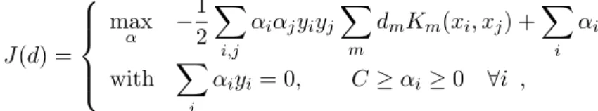
max α − 1 2 X i,j αiαjyiyjX m dmKm(xi, xj) +X i αi with X i αiyi= 0 C≥αi≥0 ∀i , (11)
which is identified as the standard SVM dual formulation using the combined kernel
K(xi, xj) =
P
mdmKm(xi, xj). Function J(d) is defined as the optimal objective value
of problem (10). Because of strong duality, J(d) is also the objective value of the dual
problem: J(d) =−1 2 X i,j α?iα?jyiyj X m dmKm(xi, xj) + X i α?i , (12)
whereα? maximizes (11). Note that the objective valueJ(d) can be obtained by any SVM
algorithm. Our method can thus take advantage of any progress in single kernel algorithms. In particular, if the SVM algorithm we use is able to handle large-scale problems, so will our MKL algorithm. Thus, the overall complexity of SimpleMKL is tied to the one of the single kernel SVM algorithm.
From now on, we assume that each Gram matrix (Km(xi, xj))i,j is positive definite,
with all eigenvalues greater than some η > 0 (to enforce this property, a small ridge may
be added to the diagonal of the Gram matrices). This implies that, for any admissible
value of d, the dual problem is strictly concave with convexity parameter η (Lemar´echal
and Sagastizabal, 1997). In turn, this strict concavity property ensures thatα? is unique,
a characteristic that eases the analysis of the differentiability of J(·).
Existence and computation of derivatives of optimal value functions such as J(·) have
been largely discussed in the literature. For our purpose, the appropriate reference is Theorem 4.1 in Bonnans and Shapiro (1998), which has already been applied by Chapelle et al. (2002) for tuning squared-hinge loss SVM. This theorem is reproduced in the appendix
the unicity of α?, and by the differentiability of the objective function that gives J(d).
Furthermore, the derivatives of J(d) can be computed as if α? were not to depend on d.
Thus, by simple differentiation of the dual function (11) with respect todm, we have:
∂J ∂dm =− 1 2 X i,j α?iα?jyiyjKm(xi, xj) ∀m . (13)
We will see in the sequel that the applicability of this theorem can be extended to other
SVM problems. Note that complexity of the gradient computation is of the order ofm·n2
SV,
withnSV being the number of support vectors for the currentd.
3.2 Reduced gradient algorithm
The optimization problem we have to deal with in (9) is a non-linear objective function with constraints over the simplex. With our positivity assumption on the kernel matrices,
J(·) is convex and differentiable with Lipschitz gradient (Lemar´echal and Sagastizabal,
1997). The approach we use for solving this problem is a reduced gradient method, which converges for such functions (Luenberger, 1984).
Once the gradient ofJ(d) is computed,dis updated by using a descent direction ensuring
that the equality constraint and the non-negativity constraints on d are satisfied. We
handle the equality constraint by computing the reduced gradient (Luenberger, 1984, Chap.
11). Let dµ be a non-zero entry of d, the reduced gradient of J(d), denoted ∇redJ, has
components: [∇redJ]m= ∂d∂J m − ∂J ∂dµ ∀m6=µ , and [∇redJ]µ= X m6=µ µ ∂J ∂dµ− ∂J ∂dm ¶ .
We chose µ to be the index of the largest component of vector d, for better numerical
stability (Bonnans, 2006).
The positivity constraints have also to be taken into account in the descent direction.
Since we want to minimizeJ(·),−∇redJ is a descent direction. However, if there is an index
m such that dm = 0 and [∇redJ]m > 0, using this direction would violate the positivity
constraint for dm. Hence, the descent direction for that component is set to 0. This gives
the descent direction for updating das
Dm = 0 ifdm= 0 and ∂dm∂J −∂dµ∂J >0 − ∂J ∂dm + ∂J ∂dµ ifdm>0 and m6=µ X g6=µ,dν>0 µ ∂J ∂dν − ∂J ∂dµ ¶ form=µ . (14)
The usual updating scheme isd←d+γD , whereγ is the step size. Here, as detailed in
Algorithm 1, we go one step beyond: once a descent directionDhas been computed, we first
look for the maximal admissible step size in that direction and check whether the objective value decreases or not. The maximal admissible step size corresponds to a component, say
dν, set to zero. If the objective value decreases,dis updated, we setDν = 0 and normalizeD
Algorithm 1 SimpleMKL algorithm
set dm = M1 form= 1, . . . , M
while stopping criterion not met do
computeJ(d) by using an SVM solver withK =PmdmKm
compute ∂d∂Jm form= 1, . . . , M and descent directionD (14). setµ= argmax
m dm,J
†= 0,d†=d,D†=D whileJ†< J(d) do{descent direction update}
d=d†,D=D† ν = argmin {m|Dm<0} −dm/Dm,γmax=−dν/Dν d†=d+γ maxD,D†µ=Dµ−Dν,D†ν = 0
computeJ† by using an SVM solver with K=P
md†mKm
end while
line search alongDforγ ∈[0, γmax]{calls an SVM solver for eachγ trial value}
d←d+γD end while
stops decreasing. At this point, we look for the optimal step sizeγ, which is determined by
using a one-dimensional line search, with proper stopping criterion, such as Armijo’s rule, to ensure global convergence.
In this algorithm, computing the descent direction and the line search are based on the
evaluation of the objective function J(·), which requires solving an SVM problem. This
may seem very costly but, for small variations of d, learning is very fast when the SVM
solver is initialized with the previous values of α? (DeCoste and Wagstaff., 2000). Note
that the gradient of the cost function is not computed after each update of the weight
vectord. Instead, we take advantage of an easily updated descent direction as long as the
objective value decreases. We will see in the numerical experiments that this approach saves a substantial amount of computation time compared to the usual update scheme
where the descent direction is recomputed after each update of d. Note that we have also
investigated gradient projection algorithms (Bertsekas, 1999, Chap 2.3), but this turned out to be slightly less efficient than the proposed approach, and we will not report these results. The algorithm is terminated when a stopping criterion is met. This stopping criterion
can be either based on the duality gap, the KKT conditions, the variation of d between
two consecutive steps or, even more simply, on a maximal number of iterations. Our implementation, based on the duality gap, is detailed in the forthcoming section.
3.3 Optimality conditions
In a convex constrained optimization algorithm such as the one we are considering, we have the opportunity to check for proper optimality conditions such as the KKT conditions or the duality gap (the difference between primal and dual objective values), which should be zero at the optimum. From the primal and dual objectives provided respectively in (2) and (8), the MKL duality gap is
DualGap =J(d?)−X i α?i +1 2maxm X i,j α?iα?jyiyjKm(xi, xj) , , whered? and {α?
i}are optimal primal and dual variables, andJ(d?) depends implicitly on
optimal primal variables {f?
m}, b? and {ξi?}. If J(d?) has been obtained through the dual
problem (11), then this MKL duality gap can also be computed from the single kernel SVM
algorithm duality gap DGSVM. Indeed, equation (12) holds only when the single kernel
SVM algorithm returns an exact solution withDGSVM= 0. Otherwise, we have
DGSVM=J(d?) +12 X i,j α?iαj?yiyj X m d?mKm(xi, xj)− X i α?i
then the MKL duality gap becomes
DualGap =DGSVM−1 2 X i,j α?iα?jyiyjX m d?mKm(xi, xj) +1 2maxm X i,j α?iα?jyiyjKm(xi, xj) .
Hence, it can be obtained with a small additional computational cost compared to the SVM duality gap.
In iterative procedures, it is common to stop the algorithm when the optimality
condi-tions are respected up to a tolerance thresholdε. Obviously, SimpleMKL has no impact on
DGSVM, hence, one may assume, as we did here, thatDGSVM needs not to be monitored.
Consequently, we terminate the algorithm when max m X i,j α?iα?jyiyjKm(xi, xj)− X i,j α?iα?jyiyj X m d?mKm(xi, xj)≤ε . (15)
For some of the other MKL algorithms that will be presented in Section 4, the dual function may be more difficult to derive. Hence, it may be easier to rely on approximate KKT conditions as a stopping criterion. For the general MKL problem (9), the first order optimality conditions are obtained through the KKT conditions:
∂J
∂dm +λ−ηm = 0 ∀m ηm·dm = 0 ∀m ,
whereλand{ηm}are respectively the Lagrange multipliers for the equality and inequality
constraints of (9). These KKT conditions imply
∂J
∂dm = −λ ifdm>0 ∂J
∂dm ≥ −λ ifdm= 0 .
However, as Algorithm 1 is not based on the Lagrangian formulation of problem (9),λ
is not computed. Hence, we derive approximate necessary optimality conditions to be used
for termination criterion. Let’s define dJmin anddJmax as
dJmin= min {dm|dm>0}
∂J
∂dm and dJmax={dm|dm>max 0} ∂J ∂dm ,
then, the necessary optimality conditions are approximated by the following termination conditions:
|dJmin−dJmax| ≤ε and ∂d∂J m
≥dJmax ifdm = 0
In other words, we are considered at the optimum when the gradient components for all
positive dm lie in a ε-tube and when all gradient components for vanishingdm are outside
this tube. Note that these approximate necessary optimality conditions are available right
away for any differentiable objective function J(d).
3.4 Cutting Planes, Steepest Descent and Computational Complexity
As we stated in the introduction, several algorithms have been proposed for solving the original MKL problem defined by Lanckriet et al. (2004b). All these algorithms are based on equivalent formulations of the same dual problem; they all aim at providing a pair of optimal vectors (d, α).
In this subsection, we contrast SimpleMKL with its closest relative, the SILP algorithm of Sonnenburg et al. (2005, 2006). Indeed, from an implementation point of view, the two algorithms are alike, since they are wrapping a standard single kernel SVM algorithm. This feature makes both algorithms very easy to implement. They, however, differ in
computational efficiency, because the kernel weights dm are optimized in quite different
ways, as detailed below.
Let us first recall that our differentiable function J(d) is defined as:
J(d) = max α − 1 2 X i,j αiαjyiyjX m dmKm(xi, xj) +X i αi with X i αiyi= 0, C≥αi ≥0 ∀i ,
and both algorithms aim at minimizing this differentiable function. However, using a SILP approach in this case, does not take advantage of the smoothness of the objective function.
The SILP algorithm of Sonnenburg et al. (2006) is acutting planemethod to minimizeJ
with respect tod. For each value ofd, the bestαis found and leads to an affine lower bound
on J(d). The number of lower bounding affine functions increases as more (d, α) pairs are
computed, and the next candidate vectordis the minimizer of the current lower bound on
J(d), that is, the maximum over all the affine functions. Cutting planes method do converge
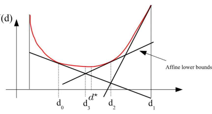
but they are known for their instability, notably when the number of lower-bounding affine functions is small: the approximation of the objective function is then loose and the iterates may oscillate (Bonnans et al., 2003). Our steepest descent approach, with the proposed line search, does not suffer from instability since we have a differentiable function to minimize. Figure 1 illustrates the behaviour of both algorithms in a simple case, with oscillations for cutting planes and direct convergence for gradient descent.
Section 5 evaluates how these oscillations impact on the computational time of the SILP algorithm on several examples. These experiments show that our algorithm needs less costly gradient computations. Conversely, the line search in the gradient base approach requires more SVM retrainings in the process of querying the objective function. However,
Figure 1: Illustrating three iterations of the SILP algorithm and a gradient descent algo-rithm for a one-dimensional problem. This dimensionality is not representative of the MKL framework, but our aim is to illustrate the typical oscillations of cutting planes around the optimal solution (with iteratesd0 tod3). Note that computing an affine lower bound at a given d requires a gradient computation. Provided the step size is chosen correctly, gradient descent converges directly towards the optimal solution without overshooting (fromd0 tod?).
the computation time per SVM training is considerably reduced, since the gradient based
approach produces estimates ofdon a smooth trajectory, so that the previous SVM solution
provides a good guess for the current SVM training. In SILP, with the oscillatory subsequent
approximations ofd?, the benefit of warm-start training severely decreases.
3.5 Convergence Analysis
In this paragraph, we briefly discuss the convergence of the algorithm we propose. We first suppose that problem (10) is always exactly solved, which means that the duality gap of such problem is 0. With such conditions, the gradient computation in (13) is exact and thus our algorithm performs reduced gradient descent on a continuously differentiable function
J(·) (remember that we have assumed that the kernel matrices are positive definite) defined
on the simplex {d|Pmdm = 1, dm ≥ 0}, which does converge to the global minimum of
J (Luenberger, 1984).
However, in practice, problem (10) is not solved exactly since most SVM algorithms
will stop when the duality gap is smaller than a given ε. In this case, the convergence of
our projected gradient method is no more guaranteed by standard arguments. Indeed, the
output of the approximately solved SVM leads only to an ε-subgradient (Bonnans et al.,
2003; Bach et al., 2004a). This situation is more difficult to analyze and we plan to address it thoroughly in future work (see for instance D’Aspremont (2008) for an example of such analysis in a similar context).
4. Extensions
In this section, we discuss how the proposed algorithm can be simply extended to other SVM algorithms such as SVM regression, one-class SVM or pairwise multiclass SVM algo-rithms. More generally, we will discuss other loss functions that can be used within our MKL algorithms.
4.1 Extensions to other SVM Algorithms
The algorithm we described in the previous section focuses on binary classification SVMs, but it is worth noting that our MKL algorithm can be extended to other SVM
algorithms with only little changes. For SVM regression with theε-insensitive loss, or
clus-tering with the one-class soft margin loss, the problem only changes in the definition of the
objective function J(d) in (10).
For SVM regression (Vapnik et al., 1997; Sch¨olkopf and Smola, 2001), we have
J(d) = min fm,b,ξi 1 2 X m 1 dmkfmk 2 Hm+C X i (ξi+ξ∗i) s.t. yi− X m fm(xi)−b≤ε+ξi ∀i X m fm(xi) +b−yi≤ε+ξi∗ ∀i ξi ≥0, ξi∗≤0 ∀i , (16)
and for one-class SVMs (Sch¨olkopf and Smola, 2001), we have:
J(d) = min fm,b,ξi 1 2 X m 1 dmkfmk 2 Hm+ 1 ν` X i ξi−b s.t. X m fm(xi)≥b−ξi ξi ≥0 . (17)
Again,J(d) can be defined according to the dual functions of these two optimization
prob-lems, which are respectively
J(d) = max α,β X i (βi−αi)yi−ε X i (βi+αi)−12 X i,j (βi−αi)(βj−αj) X m dmKm(xi, xj) with X i (βi−αi) = 0 0≤αi , βi ≤C, ∀i , (18) and J(d) = max α − 1 2 X i,j αiαjX m dmKm(xi, xj) with 0≤αi ≤ 1 ν` ∀i X i αi = 1 , (19)
where{αi} and {βi} are Lagrange multipliers.
Then, as long as J(d) is differentiable, a property strictly related to the strict concavity
of its dual function, our descent algorithm can still be applied. The main effort for the
extension of our algorithm is the evaluation ofJ(d) and the computation of its derivatives.
Like for binary classification SVM,J(d) can be computed by means of efficient off-the-shelf
SVM solvers and the gradient of J(d) is easily obtained through the dual problems. For
SVM regression, we have: ∂J ∂dm =− 1 2 X i,j (βi?−α?i)(βj?−α?j)Km(xi, xj) ∀m , (20)
and for one-class SVM, we have:
∂J ∂dm =− 1 2 X i,j α?iαj?Km(xi, xj) ∀m , (21) where α?
i and β?i are the optimal values of the Lagrange multipliers. These examples
illustrate that extending SimpleMKL to other SVM problems is rather straighforward. This
observation is valid for other SVM algorithms (based for instance on the ν parameter, a
squared hinge loss or squared-ε tube) that we do not detail here. Again, our algorithm
can be used providedJ(d) is differentiable, by plugging in the algorithm the function that
evaluates the objective value J(d) and its gradient. Of course, the duality gap may be
considered as a stopping criterion if it can be computed.
4.2 Multiclass Multiple Kernel Learning
With SVMs, multiclass problems are customarily solved by combining several binary
classifiers. The well-known one-against-all and one-against-one approaches are the two
most common ways for building a multiclass decision function based on pairwise decision functions. Multiclass SVM may also be defined right away as the solution of a global optimization problem (Weston and Watkins, 1999; Crammer and Singer, 2001), that may also be addressed with structured-output SVM (Tsochantaridis et al., 2005). Very recently, an MKL algorithm based on structured-output SVM has been proposed by Zien and Ong (2007). This work extends the work of Sonnenburg et al. (2006) to multiclass problems, with an MKL implementation still based on a QCQP or SILP approach.
Several works have compared the performance of multiclass SVM algorithms (Duan and Keerthi, 2005; Hsu and Lin, 2002; Rifkin and Klautau, 2004). In this subsection, we do not deal with this aspect; we explain how SimpleMKL can be extended to pairwise SVM multiclass implementations. The problem of applying our algorithm to structured-output SVM will be briefly discussed later.
Suppose we have a multiclass problem with P classes. For a one-against-all multiclass
SVM, we need to trainP binary SVM classifiers, where thep-th classifier is trained by
con-sidering all examples of classpas positive examples while all other examples are considered
negative. For aone-against-one multiclass problem,P(P−1)/2 binary SVM classifiers are
built from all pairs of distinct classes. Our multiclass MKL extension of SimpleMKL differs
for the combination of kernels thatjointly optimizes all the pairwise decision functions, the
objective function we want to optimize according to the kernel weights{dm} is:
J(d) =X
p∈P
Jp(d) ,
whereP is the set of all pairs to be considered, andJp(d) is the binary SVM objective value
for the classification problem pertaining to pairp.
Once the new objective function is defined, the lines of Algorithm 1 still apply. The
gradient of J(d) is still very simple to obtain, since owing to linearity, we have:
∂J ∂dm =− 1 2 X p∈P X i,j αi,p? α?j,pyiyjKm(xi, xj) ∀m , (22)
where αj,p is the Lagrange multiplier of the j-th example involved in the p-th decision
function. Note that those Lagrange multipliers can be obtained independently for each
pair.
The approach described above aims at finding the combination of kernels that jointly
optimizes all binary classification problems: this one set of features should maximize the sum of margins. Another possible and straightforward approach consists in running inde-pendently SimpleMKL for each classification task. However, this choice is likely to result in as many combinations of kernels as there are binary classifiers.
4.3 Other loss functions
Multiple kernel learning has been of great interest and since the seminal work of Lanck-riet et al. (2004b), several works on this topic have flourished. For instance, multiple kernel learning has been transposed to least-square fitting and logistic regression (Bach et al., 2004b). Independently, several authors have applied mixed-norm regularization, such as the additive spline regression model of Grandvalet and Canu (1999). This type of
regular-ization, which is now known as the group lasso, may be seen as a linear version of multiple
kernel learning (Bach, 2008). Several algorithms have been proposed for solving the group lasso problem. Some of them are based on projected gradient or on coordinate descent algorithm. However, they all consider the non-smooth version of the problem.
We previously mentioned that Zien and Ong (2007) have proposed an MKL algorithm based on structured-output SVMs. For such problem, the loss function, which differs from the usual SVM hinge loss, leads to an algorithm based on cutting planes instead of the usual QP approach.
Provided the gradient of the objective value can be obtained, our algorithm can be applied to group lasso and structured-output SVMs. The key point is whether the theorem of Bonnans et al. (2003) can be applied or not. Although we have not deeply investigated this point, we think that many problems comply with this requirement, but we leave these developments for future work.
4.4 Approximate regularization path
SimpleMKL requires the setting of the usual SVM hyperparameter C, which usually
is to compute the so-called regularization path, which describes the set of solutions as C
varies from 0 to∞.
Exact path following techniques have been derived for some specific problems like SVMs or the lasso (Hastie et al., 2004; Efron et al., 2004). Besides, regularization paths can be sampled by predictor-corrector methods (Rosset, 2004; Bach et al., 2004b).
For model selection purposes, an approximation of the regularization path may be suf-ficient. This approach has been applied for instance by Koh et al. (2007) in regularized logistic regression.
Here, we compute an approximate regularization path based on a warm-start technique.
Suppose, that for a given value ofC, we have computed the optimal (d?, α?) pair; the idea
of a warm-start is to use this solution for initializing another MKL problem with a different
value of C. In our case, we iteratively compute the solutions for decreasing values of C
(note thatα? has to be modified to be a feasible initialization of the more constrained SVM
problem).
5. Numerical experiments
In this experimental section, we essentially aim at illustrating three points. The first point is to show that our gradient descent algorithm is efficient. This is achieved by binary classification experiments, where SimpleMKL is compared to the SILP approach of Sonnen-burg et al. (2006). Then, we illustrate the usefulness of a multiple kernel learning approach in the context of regression. The examples we use are based on wavelet-based regression in which the multiple kernel learning framework naturally fits. The final experiment aims at evaluating the multiple kernel approach in a model selection problem for some multiclass problems.
5.1 Computation time
The aim of this first set of experiments is to assess the running times of SimpleMKL. 2
First, we compare with SILP regarding the time required for computing a single solution
of MKL with a givenC hyperparameter. Then, we compute an approximate regularization
path by varying C values. We finally provide hints on the expected complexity of
Sim-pleMKL, by measuring the growth of running time as the number of examples or kernels increases.
5.1.1 Time needed for reaching a single solution
In this first benchmark, we put SimpleMKL and SILP side by side, for a fixed value
of the hyperparameter C (C = 100). This procedure, which does not take into account a
proper model selection procedure, is not representative of the typical use of SVMs. It is however relevant for the purpose of comparing algorithmic issues.
The evaluation is made on five datasets from the UCI repository: Liver, Wpbc,
Iono-sphere,Pima,Sonar (Blake and Merz, 1998). The candidate kernels are:
• Gaussian kernels with 10 different bandwidthsσ, on all variables and on each single variable;
• polynomial kernels of degree 1 to 3, again on all and each single variable.
All kernel matrices have been normalized to unit trace, and are precomputed prior to running the algorithms.
Both SimpleMKL and SILP wrap an SVM dual solver based on SimpleSVM, an active constraints method written in Matlab (Canu et al., 2003). The descent procedure of Sim-pleMKL is also implemented in Matlab, whereas the linear programming involved in SILP is implemented in the publicly available toolbox LPSOLVE (Berkelaar et al., 2004).
For a fair comparison, we use the same stopping criterion for both algorithms. They
halt when, either the duality gap is lower than 0.01, or the number of iterations exceeds
2000. Quantitatively, the displayed results differ from the preliminary version of this work, where the stopping criterion was based on the stabilization of the weights, but they are qualitatively similar (Rakotomamonjy et al., 2007).
For each dataset, the algorithms were run 20 times with different train and test sets (70% of the examples for training and 30% for testing). Training examples were normalized to zero mean and unit variance.
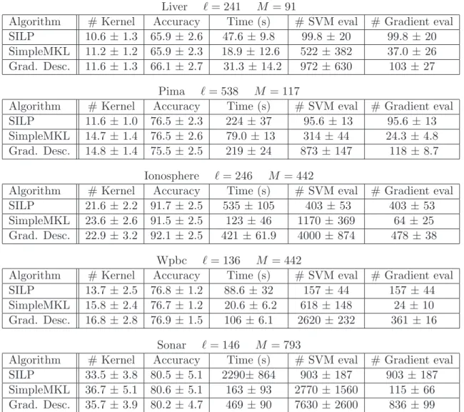
In Table 1, we report different performance measures: accuracy, number of selected kernels and running time. As the latter is mainly spent in querying the SVM solver and in
computing the gradient of J with respect tod, the number of calls to these two routines is
also reported.
Both algorithms are nearly identical in performance accuracy. Their number of selected kernels are of same magnitude, although SimpleMKL tends to select 10 to 20% more ker-nels. As both algorithms address the same convex optimization problem, with convergent methods starting from the same initialization, the observed differences are only due to the inaccuracy of the solution when the stopping criterion is met. Hence, the trajectories chosen by each algorithm for reaching the solution, detailed in Section 3.4, explain the differences
in the number of selected kernels. The updates of dm based on the descent algorithm of
SimpleMKL are rather conservative (small steps departing from 1/M for all dm), whereas
the oscillations of cutting planes are likely to favor extreme solutions, hitting the edges of the simplex.
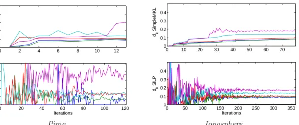
This explanation is corroborated by Figure 2, which compares the behavior of the dm
coefficients through time. The instability of SILP is clearly visible, with very high oscilla-tions in the first iteraoscilla-tions and a noticeable residual noise in the long run. In comparison, the trajectories for SimpleSVM are much smoother.
If we now look at the overall difference in computation time reported in Table 1, clearly, on all data sets, SimpleSVM is faster than SILP, with an average gain factor of about 5. Furthermore, the larger the number of kernels is, the larger the speed gain we achieve. Looking at the last column of Table 1, we see that the main reason for improvement is that SimpleMKL converges in fewer iterations (that is, gradient computations). It may seem surprising that this gain is not conterbalanced by the fact that SimpleMKL requires many more calls to the SVM solver (on average, about 4 times). As we stated in Section 3.4, when the number of kernels is large, computing the gradient may be expensive compared to SVM retraining with warm-start techniques.
Table 1: Average performance measures for the two MKL algorithms and a plain gradient descent algorithm.
Liver `= 241 M = 91
Algorithm # Kernel Accuracy Time (s) # SVM eval # Gradient eval SILP 10.6 ±1.3 65.9 ±2.6 47.6 ±9.8 99.8 ±20 99.8±20 SimpleMKL 11.2 ±1.2 65.9 ±2.3 18.9±12.6 522± 382 37.0±26 Grad. Desc. 11.6 ±1.3 66.1 ±2.7 31.3 ±14.2 972± 630 103±27
Pima `= 538 M = 117
Algorithm # Kernel Accuracy Time (s) # SVM eval # Gradient eval SILP 11.6 ±1.0 76.5 ±2.3 224±37 95.6 ±13 95.6±13 SimpleMKL 14.7 ±1.4 76.5 ±2.6 79.0 ±13 314±44 24.3 ±4.8 Grad. Desc. 14.8 ±1.4 75.5 ±2.5 219±24 873± 147 118±8.7
Ionosphere `= 246 M = 442
Algorithm # Kernel Accuracy Time (s) # SVM eval # Gradient eval SILP 21.6 ±2.2 91.7 ±2.5 535±105 403±53 403±53 SimpleMKL 23.6 ±2.6 91.5 ±2.5 123±46 1170 ±369 64± 25 Grad. Desc. 22.9 ±3.2 92.1 ±2.5 421±61.9 4000 ±874 478±38
Wpbc `= 136 M = 442
Algorithm # Kernel Accuracy Time (s) # SVM eval # Gradient eval SILP 13.7 ±2.5 76.8 ±1.2 88.6 ±32 157±44 157±44 SimpleMKL 15.8 ±2.4 76.7 ±1.2 20.6± 6.2 618± 148 24± 10 Grad. Desc. 16.8 ±2.8 76.9 ±1.5 106± 6.1 2620 ±232 361±16
Sonar `= 146 M = 793
Algorithm # Kernel Accuracy Time (s) # SVM eval # Gradient eval SILP 33.5 ±3.8 80.5 ±5.1 2290±864 903± 187 903±187 SimpleMKL 36.7 ±5.1 80.6 ±5.1 163±93 2770± 1560 115±66 Grad. Desc. 35.7 ±3.9 80.2 ±4.7 469±90 7630± 2600 836±99
0 2 4 6 8 10 12 0 0.1 0.2 0.3 0.4 dk SimpleMKL 0 20 40 60 80 100 120 0 0.1 0.2 0.3 0.4 Iterations dk SILP 0 10 20 30 40 50 60 70 0 0.1 0.2 0.3 0.4 dk SimpleMKL 0 50 100 150 200 250 300 350 0 0.1 0.2 0.3 0.4 Iterations dk SILP Pima Ionosphere
Figure 2: Evolution of the five largest weightsdmfor SimpleMKL and SILP; left row: Pima; right row: Ionosphere.
To understand why, with this large number of calls to the SVM solver, SimpleMKL is still much faster than SILP, we have to look back at Figure 2. On the one hand, the large
variations in subsequentsdm values for SILP, entail that subsequent SVM problems are not
likely to have similar solutions: a warm-start call to the SVM solver does not help much.
On the other hand, with the smooth trajectories ofdm in SimpleMKL, the previous SVM
solution is often a good guess for the current problem: a warm-start call to the SVM solver results in much less computation than a call from scratch.
Table 1 also shows the results obtained when replacing the update scheme described
in Algorithm 1 by a usual reduced gradient update, which, at each iteration, modifies d
by computing the optimal step size on the descent direction D (14). The training of this
variant is considerably slower than SimpleMKL and is only slightly better than SILP. We see that the gradient descent updates require many more calls to the SVM solver and a number of gradient computations comparable with SILP. Note that, compared to SILP, the numerous additional calls to the SVM solver have not a drastic effect on running time. The gradient updates are stable, so that they can benefit from warm-start contrary to SILP.
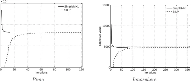
To end this first series of experiments, Figure 3 depicts the evolution of the objective function for the data sets that were used in Figure 2. Besides the fact that SILP needs more iterations for achieving a good approximation of the final solution, it is worth noting that the objective values rapidly reach their steady state while still being far from convergence,
whendm values are far from being settled. Thus, monitoring objective values is not suitable
to assess convergence.
5.1.2 Time needed for getting an approximate regularization path
In practice, the optimal value of Cis unknown, and one has to solve several SVM
prob-lems, spanning a wide range ofCvalues, before choosing a solution according to some model
0 20 40 60 80 100 120 2 2.5 3 3.5x 10 4 Objective value Iterations SimpleMKL SILP 0 50 100 150 200 250 300 350 0 5000 10000 15000 Objective value Iterations SimpleMKL SILP Pima Ionosphere
Figure 3: Evolution of the objective values for SimpleSVM and SILP; left row: Pima; right row: Ionosphere.
of the running times of SimpleMKL and SILP, in a series of experiments that include the
search for a sensible value ofC.
In this new benchmark, we use the same data sets as in the previous experiments, with the same kernel settings. The task is only changed in the respect that we now evaluate the running times needed by both algorithms to compute an approximate regularization path. For both algorithms, we use a simple warm-start technique, which consists in using the
optimal solutions {d?
m}and {α?i} obtained for a given C to initialize a new MKL problem
withC+ ∆C(DeCoste and Wagstaff., 2000). As described in Section 4.4, we start from the
largest C and then approximate the regularization path by decreasing its value. The set of
C values is obtained by evenly sampling the interval [0.01,1000] on a logarithmic scale.
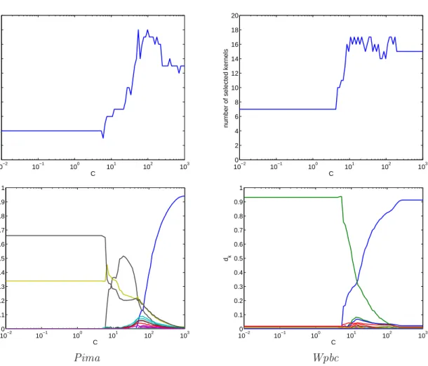
Figure 4 shows the variations of the number of selected kernels and the values ofdalong
the regularization path for the Pima and Wpbc datasets. The number of kernels is not a
monotone function ofC: for small values ofC, the number of kernels is somewhat constant,
then, it rises rapidly. There is a small overshooth before reaching a plateau corresponding
to very high values ofC. This trend is similar for the number of leading terms in the kernel
weight vectord. Both phenomenon were observed consistently over the datasets we used.
Table 2 displays the average computation time (over 10 runs) required for building the approximate regularization path. As previously, SimpleMKL is more efficient than SILP, with a gain factor increasing with the number of kernels in the combination. The range
of gain factors, from 5.9 to 23, is even more impressive than in the previous benchmark.
SimpleMKL benefits from the continuity of solutions along the regularization path, whereas SILP does not take advantage of warm starts. Even provided with a good initialization, it needs many cutting planes to stabilize.
100−2 10−1 100 101 102 103 2 4 6 8 10 12 14 16 18 20 C
number of selected kernels
100−2 10−1 100 101 102 103 2 4 6 8 10 12 14 16 18 20 C
number of selected kernels
10−2 10−1 100 101 102 103 0 0.1 0.2 0.3 0.4 0.5 0.6 0.7 0.8 0.9 1 C dk 10−2 10−1 100 101 102 103 0 0.1 0.2 0.3 0.4 0.5 0.6 0.7 0.8 0.9 1 C dk Pima Wpbc
Figure 4: Regularization paths for dm and the number of selected kernels versus C; left row: Pima; right row: Wpbc.
Table 2: Average computation time (in seconds) for getting an approximate regularization path. For the Sonar data set, SILP was extremely slow, so that regularization path was computed only once.
Dataset SimpleMKL SILP Ratio Liver 148±37 875±125 5.9 Pima 1030±195 6070 ±1430 5.9 Ionosphere 1290±927 8840 ±1850 6.8
Wpbc 88 ±16 2040 ±544 23
5.1.3 More on SimpleMKL running times
Here, we provide an empirical assessment of the expected complexity of SimpleMKL on different data sets from the UCI repository. We first look at the situation where kernel matrices can be pre-computed and stored in memory, before reporting experiments where the memory are too high, leading to repeated kernel evaluations.
In a first set of experiments, we use Gaussian kernels, computed on random subsets of variables and with random width. These kernels are precomputed and stored in memory, and we report the average CPU running times obtained from 20 runs differing in the random draw of training examples. The stopping criterion is the same as in the previous section: a
relative duality gap less thanε= 0.01.
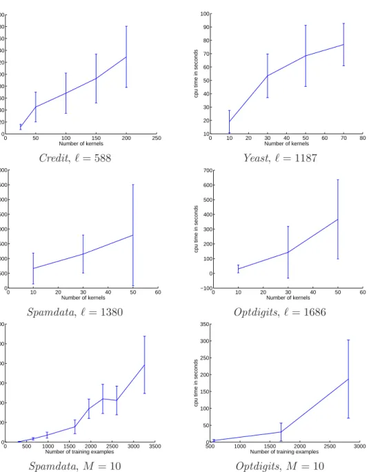
The first two rows of Figure 5 depicts the growth of computation time as the num-ber of kernel increases. We observe a nearly linear trend for the four learning problems. This growth rate could be expected considering the linear convergence property of gradient techniques, but the absence of overhead is valuable.
The last row of Figure 5 depicts the growth of computation time as the number of examples increases. Here, the number of kernels is set to 10. In these plots, the observed trend is clearly superlinear. Again, this trend could be expected, considering that SVM expected training times are superlinear in the number of training examples. As we already mentioned, the complexity of SimpleMKL is tightly linked to the one of SVM training (for some examples of single kernel SVM running time, one can refer to the work of Loosli and Canu (2007)).
When all the kernels used for MKL cannot be stored in memory, one can resort to a decomposition method. Table 3 reports the average computation times, over 10 runs, in this more difficult situation. The large-scale SVM scheme of Joachims (1999) has been imple-mented, with basis kernels recomputed whenever needed. This approach is computationally expensive but goes with no memory limit. For these experiments, the stopping criterion is
based on the variation of the weightsdm. As shown in Figure 2, the kernel weights rapidly
reach a steady state and many iterations are spent for fine tuning the weight and reach the duality gap tolerance. Here, we trade the optimality guarantees provided by the duality gap for substantial computational time savings. The algorithm terminates when the kernel
weights variation is lower than 0.001.
Results reported in Table 3 just aim at showing that medium and large-scale situations can be handled by SimpleMKL. Note that Sonnenburg et al. (2006) have run a modified version of their SILP algorithm on a larger scale datasets. However, for such experiments, they have taken advantage of some specific feature map properties. And, as they stated, for general cases where kernel matrices are dense, they have to rely on the SILP algorithm we used in this section for efficiency comparison .
5.2 Multiple kernel regression examples
Several research papers have already claimed that using multiple kernel learning can lead to better generalization performances in some classification problems (Lanckriet et al., 2004a; Zien and Ong, 2007; Harchaoui and Bach, 2007). This next experiment aims at illustrating this point but in the context of regression. The problem we deal with is a classical univariate regression problem where the design points are irregular (D’Amato et al.,
0 50 100 150 200 250 0 20 40 60 80 100 120 140 160 180 200 Number of kernels
cpu time in seconds
0 10 20 30 40 50 60 70 80 10 20 30 40 50 60 70 80 90 100 Number of kernels
cpu time in seconds
Credit,`= 588 Yeast,`= 1187 0 10 20 30 40 50 60 0 500 1000 1500 2000 2500 3000 3500 4000 Number of kernels
cpu time in seconds
0 10 20 30 40 50 60 −100 0 100 200 300 400 500 600 700 Number of kernels
cpu time in seconds
Spamdata,`= 1380 Optdigits,`= 1686 0 500 1000 1500 2000 2500 3000 3500 0 100 200 300 400 500 600
Number of training examples
cpu time in seconds
500 1000 1500 2000 2500 3000 0 50 100 150 200 250 300 350
Number of training examples
cpu time in seconds
Spamdata,M = 10 Optdigits,M = 10
Figure 5: SimpleMKL average computation times for different datasets; top two rows: num-ber of training examples fixed, numnum-ber of kernels varying; bottom row: numnum-ber of training examples varying, number of kernels fixed.
Table 3: Average computation time needed by SimpleSVM using decomposition methods. Dataset Nb Examples # Kernel Accuracy (%) Time (s)
Yeast 1335 22 77.25 1130
2006). Furthermore, according to equation (16), we look for the regression function f(x) as a linear combination of functions each belonging to a wavelet based reproducing kernel Hilbert space.
The algorithm we use is a classical SVM regression algorithm with multiple kernels where each kernel is built from a set of wavelets. These kernels have been obtained according to the expression: K(x, x0) =X j X s 1 2jψj,s(x)ψj,s(x0)
where ψ(·) is a mother wavelet and j,s are respectively the dilation and translation
pa-rameters of the waveletψj,s(·). The theoretical details on how such kernels can been built
are available in D’Amato et al. (2006); Rakotomamonjy and Canu (2005); Rakotomamonjy et al. (2005).
Our hope when using multiple kernel learning in this context is to capture the multiscale structure of the target function. Hence, each kernel involved in the combination should be weighted accordingly to its correlation to the target function. Furthermore, such a kernel has to be built according to the multiscale structure we wish to capture. In this experiment, we have used three different choices of multiple kernels setting. Suppose we have a set of wavelets with j∈[jmin, jmax] and s∈∈[smin, smax].
First of all, we have build a single kernel from all the wavelets according to the above equation. Then we have created kernels from all wavelets of a given scale (dilation)
KDil,J(x, x0) = smaxX
s=smin
1
2jψJ,s(x)ψJ,s(x0) ∀J ∈[jmin, jmax]
and lastly, we have a set of kernels, where each kernel is built from wavelets located at a given scale and given time-location:
KDil−T rans,J,S(x, x0) = X s=S 1 2jψJ,s(x)ψJ,s(x 0) ∀J ∈[j min, jmax]
where S is a given set of translation parameter. These sets are built by splitting the full
translation parameters index in contiguous and non-overlapping index. The mother wavelet
we used is a Symmlet Daubechies wavelet with 6 vanishing moments. The resolution levels
of the wavelet goes from jmin =−3 to jmin = 6. According to these settings, we have 10
dilation kernels and 48 dilation-translation kernels.
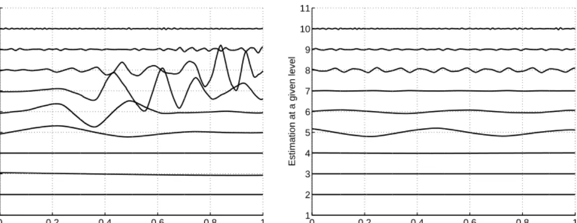
We applied this MKL SVM regression algorithm to simulated datasets which are well-known functions in the wavelet literature (Antoniadis and Fan, 2001). Each signal length is 512 and a Gaussian independent random has been added to each signal so that the signal to noise ratio is equal to 5. Examples of the true signals and their noisy versions are displayed
in Figure 6. Note that the LinChirp and Wave signals present some multiscale features
that should suit well to an MKL approach.
Performance of the different multiple kernel settings have been compared according to the following experimental setting. For each training signal, we have estimated the
regularization parameterCof the MKL SVM regression by means of a validation procedure.
0 0.2 0.4 0.6 0.8 1 −1 −0.5 0 0.5 1 LinChirp 0 0.2 0.4 0.6 0.8 1 −2 −1 0 1 2 x 0 0.2 0.4 0.6 0.8 1 0.2 0.4 0.6 0.8 1 Wave 0 0.2 0.4 0.6 0.8 1 0 0.5 1 x 0 0.2 0.4 0.6 0.8 1 0.2 0.4 0.6 0.8 1 Blocks 0 0.2 0.4 0.6 0.8 1 0 0.2 0.4 0.6 0.8 x 0 0.2 0.4 0.6 0.8 1 0.2 0.4 0.6 0.8 1 Spikes 0 0.2 0.4 0.6 0.8 1 0 0.5 1 x
Figure 6: Examples of signals to approximate in the regression problem. (top-left) LinChirp. (top-right) Wave. (bottom-left) Blocks. (bottom-right) Spikes. For each figure, the top plot depicts the true signal while the bottom one presents an example of their randomly sampled noisy versions.
means of an approximate regularization path as described in Section 4.4, we learn different
regression functions for 20 samples ofClogarithmically sampled on the interval [0.01,1000].
This is performed for 5 random draws of the learning and validation sets. TheCvalue that
gives the lowest average normalized mean-square error is considered as the optimal one.
Finally, we use all the samples of the training signal and the optimal C value to train an
MKL SVM regression. The quality of the resulting regression function is then evaluated
with respect to 1000 samples of the true signal. For all the simulations theεhas been fixed
to 0.1.
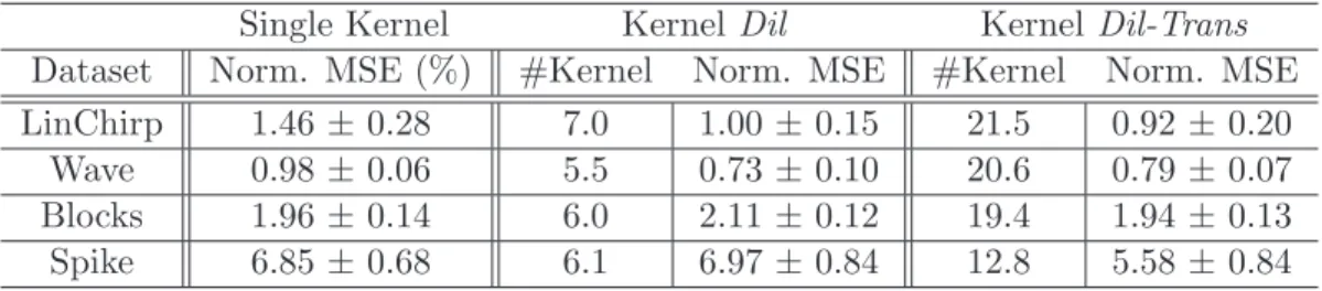
Table 4 summarizes the generalization performances achieved by the three different ker-nel settings. As expected, using a multiple kerker-nel learning setting outperforms the single kernel setting especially when the target function presents multiscale structure. This is