Predictive Performance Of Machine Learning Algorithms For Ore Reserve Estimation In Sparse And Imprecise Data

FOR ORE RESERVE ESTIMATION IN SPARSE AND IMPRECISE DATA

A THESIS

Presented to the Faculty

of the University of Alaska Fairbanks in Partial Fulfillment of the Requirements

for the Degree of

DOCTOR OF PHILOSOPHY

By

Sridhar Dutta, M. Tech

Fairbanks, Alaska August 2006

UMI Number: 3229733

INFORMATION TO USERS

The quality of this reproduction is dependent upon the quality of the copy

submitted. Broken or indistinct print, colored or poor quality illustrations and

photographs, print bleed-through, substandard margins, and improper

alignment can adversely affect reproduction.

In the unlikely event that the author did not send a complete manuscript

and there are missing pages, these will be noted. Also, if unauthorized

copyright material had to be removed, a note will indicate the deletion.

®

UMI

UMI Microform 3229733

Copyright 2006 by ProQuest Information and Learning Company.

All rights reserved. This microform edition is protected against

unauthorized copying under Title 17, United States Code.

ProQuest Information and Learning Company

300 North Zeeb Road

P.O. Box 1346

Ann Arbor, Ml 48106-1346

FOR ORE RESERVE ESTIMATION IN SPARSE AND IMPRECISE DATA RECOMMEND: APPROVED: By Sridhar Dutta W\A k ir i-li'T 'Z L

Advisory Committee Chair

ck

cl

ment C har, Mining & (

Department C har, Mining & Geological Engineering

Dean, College of Engineering and Mines

Dean of Graduate School

ABSTRACT

Traditional geostatistical estimation techniques have been used predominantly in the mining industry for the purpose o f ore reserve estimation. Determination o f mineral reserve has always posed considerable challenge to mining engineers due to geological complexities that are generally associated with the phenomenon o f ore body formation. Considerable research over the years has resulted in the development o f a number of state-of-the-art methods for the task of predictive spatial mapping such as ore reserve estimation. Recent advances in the use of the machine learning algorithms (MLA) have provided a new approach to solve the age-old problem. Therefore, this thesis is focused on the use of two MLA, viz. the neural network (NN) and support vector machine (SVM), for the purpose o f ore reserve estimation. Application o f the MLA have been elaborated with two complex drill hole datasets. The first dataset is a placer gold drill hole data characterized by high degree o f spatial variability, sparseness and noise while the second dataset is obtained from a continuous lode deposit.

The application and success o f the models developed using these MLA for the purpose of ore reserve estimation depends to a large extent on the data subsets on which they are trained and subsequently on the selection o f the appropriate model parameters. The model data subsets obtained by random data division are not desirable in sparse data conditions as it usually results in statistically dissimilar subsets, thereby reducing their applicability. Therefore, an ideal technique for data subdivision has been suggested in the thesis. Additionally, issues pertaining to the optimum model development have also been discussed.

To investigate the accuracy and the applicability o f the MLA for ore reserve estimation, their generalization ability was compared with the geostatistical ordinary kriging (OK) method. The analysis o f Mean Square Error (MSE), Mean Absolute Error (MAE), Mean Error (ME) and the coefficient o f determination (R ) as the indices of the model performance indicated that they may significantly improve the predictive ability and thereby reduce the inherent risk in ore reserve estimation.

Signature Page...i

Title Page...ii

Abstract...iii

Table of Contents...iv

List of Figure... viii

List of Tables... xii

List of Appendices...xv

Acknowledgement... xvi

Chapter 1 INTRODUCTION... 1

1.1 Ore Reserve Estimation... 1

1.2 Statement of Ore Reserve Estimation Problem... 3

1.3 Literature Review... 6

1.4 Scope of the Study... 11

Chapter 2 THEORY OF GENETIC ALGORITHMS AND KOHONEN NETWORK... 14

2.1 Genetic algorithms for data division... 14

2.2 Self Organizing Map and Data Division... 20

Chapter 3 THEORY OF SUPPORT VECTOR MACHINES... 23

3.1 Basics of Supervised Learning from Data... 23

3.2 Support Vector Machines in Regression... 25

3.2.1 Statistical Learning Theory... 26

3.2.2 Support Vector Regression...27

V

C hapter 4 ADDRESSING TH E SPARSE DATA ISSUE IN N O M E... 33

4.1 Placer Gold in Nome... 33

4.1.1 The History o f Offshore Exploration... 36

4.1.2 Problem o f Gold Reserve Estimation... 37

4.1.3 Sparse Data Problem... 38

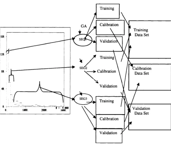
4.1.4 Data Segmentation for Data Division... 49

4.1.4.1 Data Segmentation and GA for Data Division...50

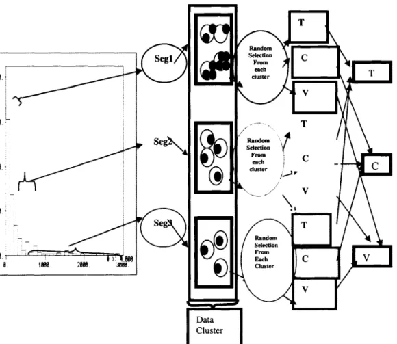
4.1.4.2 Data Segmentation and Kohonen Network for Data Division... 60

C hapter 5 NOME GOLD RESERVE ESTIM ATION USING ORIGINAL FISH B L O C K S ... 64

5.1 Geostatistical Modeling... 66

5.1.1 Ordinary Kriging for Ore Grade Estimation...66

5.1.2 OK Nome Ore Grade Estimation Results Using OK... 68

5.2 Neural Network Modeling...70

5.2.1 Neural Network for Ore Grade Estimation...70

5.2.2 Optimization of Neural Network Training...73

5.2.2.1 Local Learning Algorithms... 74

5.2.2.1.1 Standard Backpropagation Algorithm with Gradient Descent (SBP)...75

5.2.2.1.2 Backpropagation with Momentum (MBP)...76

5.2.2.1.3 Levenberg -Marquardt Algorithm (LMBP)... 76

5.2.2.2 Model Generalization...77

5.2.2.2.1 Quick Stop Training...77

5.2.2.3 Model Performance Measurement...79 Page

5.2.3 NN Nome Ore Grade Estimation Results...80

5.2.3.1 Performance o f Optimization Algorithms...81

5.3 Support Vector Machine Modeling... 91

5.3.1 SVM for Ore Grade Estim ation...91

5.3.2 SVM Nome Ore Grade Estimation Results...93

5.4 Grade Forecasting and Reserve Estimation... 100

Chapter 6 COMPARATIVE ANALYSIS OF THE ESTIMATION TECNIQUES IN A LODE DEPOSIT...106

6.1 Description o f the Study Area... 106

6.2 Model Development and Analysis of the Data...108

6.3 Results and Discussion...114

Chapter 7 NOME GOLD RESERVE ESTIMATION USING ARTIFICIAL BLOCKS...118

7.1 Clustering Algorithms...118

7.1.1 K-Means Algorithm...119

7.1.2 Fuzzy C-Means Algorithm...120

7.2 Results and Discussion...121

7.2.1 Gold Reserve Estimation...132

Chapter 8 SUMMARY AND CONCLUSIONS...136

8.1 Summary... 136

REFERENCES...142 APPENDICES...150

vii

Page

Figure 2-1: Principal stages of genetic algorithms...16

Figure 2-2: Genetic algorithms for data division...19

Figure 3-1: Dependence of VC confidence on the VC dimension...27

Figure 3-2: Bound on the test error derived in SLT...27

Figure 3-3: £ insensitivity loss function...28

Figure 3-4: Architecture of regression machine constructed by the SVM... 31

Figure 4-1: Location of the Nome area... 34

Figure 4-2: Offshore placer Gold deposit... 35

Figure 4-3: Location of drill holes in Coho block...40

Figure 4-4: Location of drill holes in Halibut block... 40

Figure 4-5: Location of drill holes in Herring block... 40

Figure 4-6: Location of drill holes in Humpy block... 40

Figure 4-7: Location of drill holes in King block... 40

Figure 4-8: Location of drill holes in Pink block... 40

Figure 4-9: Location of drill holes in Red block... 41

Figure 4-10: Location of drill holes in Silver block... 41

Figure 4-11 Location of drill holes in Tomcod block...41

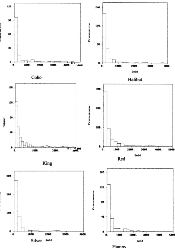
Figure 4-12: Histogram plot of Nome Gold data (various fish blocks)... 42

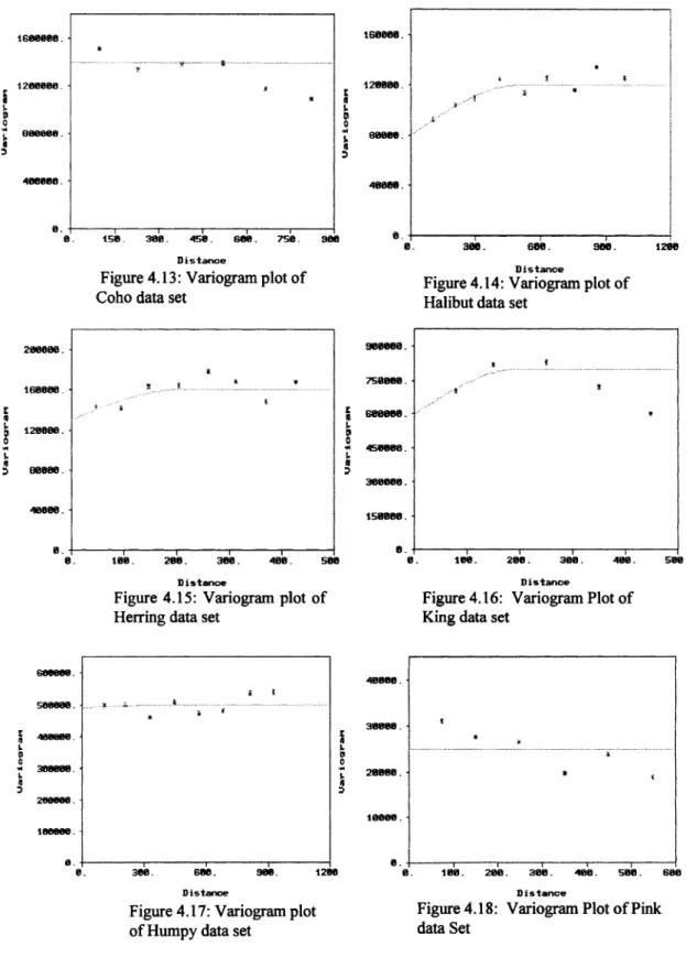
Figure 4-13: Variogram plot of Coho data set...44

Figure 4-14: Variogram plot of Halibut data set... 44

Figure 4-15: Variogram plot of Herring data set...44

Figure 4-16: Variogram plot of King data set... 44

Figure 4-17: Variogram plot of Humpy data set... 44

Figure 4-18: Variogram plot of Pink data set...44

Figure 4-19: Variogram plot of Red data set... 45

Figure 4-20: Variogram plot of Silver data set...45

Figure 4-21: Variogram plot of Tomcod data set... 45

Figure 4-22: Data segmentation and genetic algorithm for data division...53

ix

Figure 4-24: Histogram plot of Halibut data set... 56

Figure 4-25: Histogram plot o f Herring data set... 57

Figure 4-26: Histogram plot o f Humpy data set...57

Figure 4-27: Histogram plot o f King data set...58

Figure 4-28: Histogram plot of Pink data set...58

Figure 4-29: Histogram plot o f Red data set...59

Figure 4-30: Histogram plot of Silver data set...59

Figure 4-31: Histogram plot of Tomcod data set... 59

Figure 4-32: Data segmentation and kohonen network for data division...61

Figure 5-1: Neural network architecture...71

Figure 5-2: A typical profile of training and calibration error of NN model... 79

Figure 5-3a Network learning with various learning algorithms (King data) (y=4, a= .4 )... 83

Figure 5-3b Network learning with various learning algorithms (King data) (y=.4, a = 2 )...83

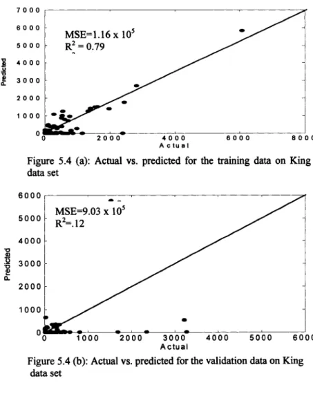
Figure 5-4a Actual vs. predicted for the training data on King data s e t...86

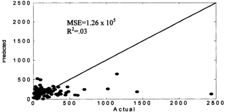
Figure 5-4b Actual vs. predicted for the validation data on King data s e t...86

Figure 5-5: Actual vs. predicted for the validation data of Coho block...88

Figure 5-6: Actual vs. predicted for the validation data of Halibut block... 88

Figure 5-7: Actual vs. predicted for the validation data of Herring block... 88

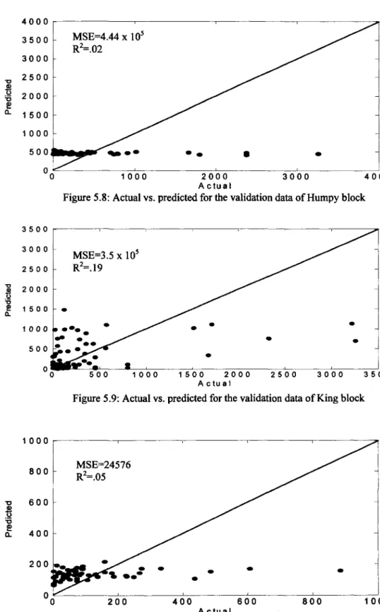
Figure 5-8: Actual vs. predicted for the validation data of Humpy block... 89

Figure 5-9: Actual vs. predicted for the validation data of King block... 89

Figure 5-10: Actual vs. predicted for the validation data of Pink block... 89

Figure 5-11: Actual vs. predicted for the validation data of Red block... 90

Figure 5-12: Actual vs. predicted for the validation data of Silver block... 90

Figure 5-13: Actual vs. predicted for the validation data of Tomcod block... 90

Figure 5-14: Effect of cost and kernel width variation on error (Pink)... 94

Figure 5-15: Effect of cost and kernel width variation on error (Red)... 94

Figure 5-16: Effect of cost and kernel width variation on error (Halibut)... 95

Figure 5-17: Effect of cost and kernel width variation on error (Herring)... 95 Page

Figure 5-18: Effect of cost and kernel width variation on error (Humpy)... 95

Figure 5-19: Effect of cost and kernel width variation on error (King)...95

Figure 5-20: Effect of cost and kernel width variation on error (Silver)... 96

Figure 5-21: Effect of cost and kernel width variation on error (Tomcod)... 96

Figure 5-22: Effect of cost and kernel width variation on error (Coho)... 96

Figure 5-23: Scatter plot for actual vs. predicted grade (Herring)...97

Figure 5-24: Scatter plot for actual vs. predicted grade (Halibut)... 97

Figure 5-25: Scatter plot for actual vs. predicted grade (Humpy)... 98

Figure 5-26: Scatter plot for actual vs. predicted grade (King)... 98

Figure 5-27: Scatter plot for actual vs. predicted grade (Pink)... 98

Figure 5-28: Scatter plot for actual vs. predicted grade (Red)... 99

Figure 5-29: Scatter plot for actual vs. predicted grade (Silver)...99

Figure 5-30: Scatter plot for actual vs. predicted grade (Tomcod)...99

Figure 5-31: Scatter plot for actual vs. predicted grade (Coho)...100

Figure 5-32: Polygonal regions formed within the Humpy block... 102

Figure 5-33: Contour plot for the predicted gold reserve (Coho)...103

Figure 5-34: Contour plot for the predicted gold reserve (Halibut)... 103

Figure 5-35: Contour plot for the predicted gold reserve (Humpy)... 103

Figure 5-36: Contour plot for the predicted gold reserve (Herring)...104

Figure 5-37: Contour plot for the predicted gold reserve (King)... 104

Figure 5-38: Contour plot for the predicted gold reserve (Pink)... 104

Figure 5-39: Contour plot for the predicted gold reserve (Red)... 105

Figure 5-40: Contour plot for the predicted gold reserve (Silver)...105

Figure 5-41: Contour plot for the predicted gold reserve (Tomcod)...105

Figure 6-1: Location of the Greens Creek Mine, Alaska... 107

Figure 6-2: Histogram plot for the Silver values... 108

Figure 6-3 Snapshot of the semi-variogram modeling on the variable Silver... 109

Figure 6-4: Ward net architecture for the NN modeling...112

Figure 6-5: Effect of the cost and kernel width on the error for silver values... 113

Figure 6-6: Variation of error with epsilon e for the variable Silver... 114

Figure 6-7: True vs. predicted (SVM)... 116 Page

xi

Figure 6-8: True vs. predicted (NN)... 116

Figure 6-9: True vs. predicted (OK)... 116

Figure 6-10: Error distribution for the Silver values (OK)... 117

Figure 6-11: Error distribution for the Silver values (NN)... 117

Figure 6-12: Error distribution for the Silver values (SVM)...117

Figure 7-1: Map showing clustered dataset using K-means algorithm... 123

Figure 7-2: Map showing clustered dataset using FCM algorithm... 124

Figure 7-3 Partitioning of the dataset in clusters using K-means and FC M ... 125

Figure 7-4: Variation of performance statistics among clusters (K-means)... 126

Figure 7-5: Variation o f performance statistics among clusters (FCM)...127

Figure 7-6: Variation in R2 for the clusters created using the K-means and FCM 128 Figure 7-7: Map showing the location of the optimal number of clusters... 129

Figure 7-8: Predicted vs. observed gold grades for the clusters by FCM... 131

Figure 7-9: Predicted gold grade (in mg/ cu.m) in cluster # 1 ... 132

Figure 7-10: Predicted gold grade (in mg/ cu.m) in cluster # 2... 132

Figure 7-11: Predicted gold grade (in mg/ cu.m) in cluster # 3... 133

Figure 7-12: Predicted gold grade (in mg/ cu.m) in cluster # 4 ... 133

Figure 7-13: Predicted gold grade (in mg/ cu.m) in cluster # 5 ... 134 Figure 7-14: Map showing zones of varying potentiality for a gold mining scenario 135

Page

Table 3-1: Basic models and their error functions...25

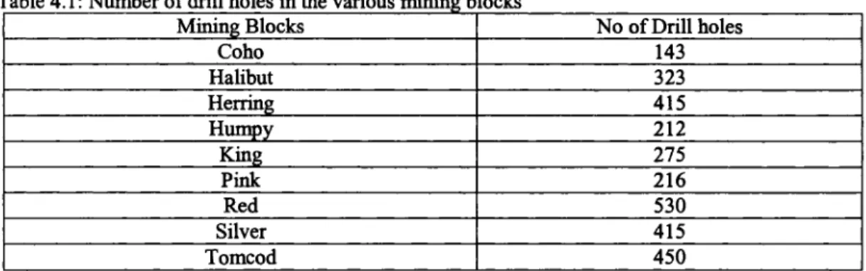
Table 4-1 Number o f drill holes in various mining blocks... 39

Table 4-2: Summary statistics o f the Nome gold datasets... 41

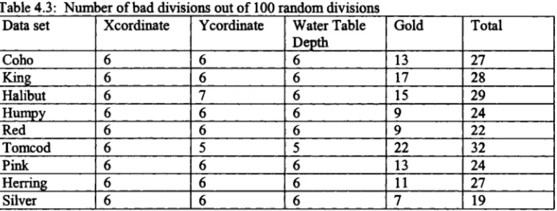
Table 4-3: Number o f bad divisions out of 100 random divisions... 48

Table 4-4: Statistical summary o f one o f the random division for Coho data set...49

Table 4-5: Statistical summary o f one o f the random division for Halibut data set... 49

Table 4-6 Statistical summary o f one o f the random division for Herring data set... 49

Table 4-7: Statistical summary o f one o f the random division for Humpy data set... 49

Table 4-8: Statistical summary o f one o f the random division for King data set...49

Table 4-9: Statistical summary o f one of the random division for Pink data set...50

Table 4-10: Statistical summary o f one o f the random division for Red data set...50

Table 4-11 Statistical summary o f one o f the random division for Silver data set.. .50

Table 4-12: Statistical summary o f one o f the random division for Tomcod data set...50

Table 4-13: Data division in King data set without data segmentation...51

(a) Genetic algorithm Table 4-13: Data division in King data set without data segmentation...52

(b) Kohonen network Table 4-14: Statistical summary o f data division using GA (Coho)...53

Table 4-15: Statistical summary o f data division using GA (Halibut)... 53

Table 4-16 Statistical summary o f data division using GA (Herring)...54 Page

xiii

Table 4-18: Statistical summary o f data division using GA (King)... 54

Table 4-19: Statistical summary o f data division using GA (Pink)... 54

Table 4-20: Statistical summary o f data division using GA (Red)... 54

Table 4-21 Statistical summary o f data division using GA (Silver)...55

Table 4-22: Statistical summary o f data division using GA (Tomcod)... 55

Table 4-23: Summary o f the data division using Kohonen network (Coho)...62

Table 4-24: Summary o f the data division using Kohonen network (Halibut)...62

Table 4-25: Summary o f the data division using Kohonen network (Herring)...62

Table 4-26 Summary o f the data division using Kohonen network (Humpy)...62

Table 4-27: Summary o f the data division using Kohonen network (King)... 62

Table 4-28: Summary o f data the division using Kohonen network (Pink)... 63

Table 4-29: Summary o f the data division using Kohonen network (Red)... 63

Table 4-30 Summary o f the data division using Kohonen network (Silver)...63

Table 4-31: Summary o f the data division using Kohonen network (Tomcod)...63

Table 5-1: Example o f drill hole data for King block... 65

Table 5-2: Number o f samples in the validation dataset for the fish blocks...66

Table 5-3: OK estimates for the fish blocks...69

Table 5-4: Number o f neurons for various datasets in NN modeling...82

Table 5-5: Performance o f various local learning algorithms... 84

Table 5-6: Generalization performance o f NN models in fish blocks...87

Table 5-7: Commonly used kernels in SVM...92

Table 5-8: Cost function and Kernel width values for the blocks... 94

Table 5-9: Performance o f SVM models for the various fish blocks...97

Table 5-10: Number o f grids inside the sampling region and in polygonal area 101 Table 5-11: Total reserve estimate for each block (in tones)...102

Table 6-1: Statistical properties o f the Greens Creek model datasets... 110

Table 6.2: Generalization performance o f the models for the variable Silver... 115

Table 6-3: Model performances based on skill values... 115 Page

Table 7-1: Number o f samples in the cluster validation datasets... 130

Table 7.2: Model performance for the optimum clusters (FCM)... 130

Table 7-3: Estimated gold reserves for the cluster b lo ck s...134

Table 7-4: Estimated density gold reserves for the cluster b lo ck s... 135 Page

XV

APPENDIX A MATLAB CODE FOR NEURAL NETWORK MODELING... 150

APPENDIX B R CODE FOR SUPPORT VECTOR MACHINE M ODELING 177

LIST OF APPENDICES

Page

ACKNOWLEDGEMENTS

This research project was funded by the Department o f Interior*s Mineral Management Service through the University o f Alaska Fairbanks’ Marine Mineral Technology Center. Dr. Sukumar Bandopadhyay, Department of Mining and Geological Engineering, University o f Alaska Fairbanks served as the principal investigator o f the project.

I would like to express my deep sense o f gratitude and heart felt thanks to my supervisor Dr. Sukumar Bandopadhyay, for his invaluable guidance, advice, encouragement, constant support and whole hearted cooperation dining the course o f my studies at UAF.

I am also grateful and express my sincere thanks to my committee members Dr. Falk Huettmann, Dr. Debasmita Misra and Dr. Rajive Ganguli for their advice, suggestions, encouragement and feedback on my work.

I specially thank Dr. Biswajit Samanta who without any hesitation always extended his help and offered suggestions whenever and wherever required. It is my pleasure to express gratitude to the staff and faculty members o f the department for their support throughout this period.

I also extend my thanks to all my friends specially Debasish, Niladri, Dinesh, Abhijit, Neil and Pratap for their pleasant company within and outside the department. It is impossible to name all the people who helped me directly or indirectly in the course of this work. Therefore, I humbly extend my words o f gratitude to all the inmates o f the department and to all others, who might think they had been helpful to me in some way or another.

Last but not the least, I sincerely thank my parents, my wife and almighty God for their love, help and support all my life.

1

CHAPTER I INTRODUCTION

1.1 Ore Reserve Estimation

The ore reserve estimation problem, essentially a statistical problem, can be stated simply as the determination o f the value (or quantity) o f the ore in unsampled areas from a set of sample data (usually drill hole samples) Xi, X2, X3, ....X n collected at specific locations within a deposit. During this process it is assumed that the samples used for the inference o f the unknown population or the underlying function responsible for the data are random and independent of each other.

The ore reserve estimation is usually a continuous process that begins during the exploration phase o f a project and in some cases, continues throughout the life of the mine. At the early stage when sampling is conducted in widely spaced drill hole intervals, the estimates are basically global and have low confidence. In spite o f the low confidence this is the first step at which mineral appraisal is carried out, and the objective o f this estimation is to obtain a reasonable approximation o f the grade-tonnage curve within a deposit confined by recognizable geological boundaries or a mineralized envelope. It also clarifies if further drilling is required. In that situation secondary drill holes are drilled at closer spacing to improve reliability. During the planning phase an estimate o f the total recoverable reserves is made for various (i) cut-off grades and (ii) mining unit sizes. In this stage, the grade-tonnage curve is generated for blocks or for mining unit sizes. Based on the quality, quantity and location information o f the ore grade obtained during this stage the subsequent mine operations are planned. Whatever the goal o f reserve estimation, a reliable prediction is prerequisite for successful compilation o f a mining project. Since the accuracy o f grade estimation is one of the key factors for effective

m ining p lanning, design, and grade control, the estimation methodologies have

undergone a great deal o f improvement, keeping pace with the advancement of

technology. There are a number o f methodologies (Dutta et al., 2003; Dutta et al., 2006a; Dutta et al., 2006b; Samanta et al., 2005a, Samanta et al., 2005b) that can be used for the ore reserve estimation. The most common and widely used methods are the traditional geostatistical estimation techniques o f kriging. Typically, the aforesaid criteria of randomness and independence among the samples are rarely observed. The samples are correlated spatially and it is this spatial relationship that is incorporated in the traditional geostatistical estimation procedure. This information is contained in a tool known as the “variogram function” which describes the continuity o f the mineralization within a deposit both graphically and numerically. It can be also used to study the anisotropies, zones of influence and the variability o f the ore grade values in the deposit.

Prior to the application of geostatistics, the ore reserve estimation methods were mostly empirical in nature. They consisted of the block methods (triangular, polygonal, and irregular) and the methods of cross section (vertical, horizontal, inclined). Recent advances in computational fields brought about the methods such as inverse distance weighing (IDW), which weighs the samples inversely with the distance from the point under consideration and combines them linearly.

Apart from the IDW methods, there are a number of kriging variants which are linear estimators. The most common is the ordinary kriging (O K ) method, also known as the best linear unbiased estimator (BLUE). Unlike the other linear estimators the distinguishing feature o f the O K method lies in its ability to produce estimates with

minimum error variance. Even this best linear estimator o f OK, may not however,

perform satisfactorily under conditions of non-linearity. Under such situations, when non­ linearity is present in the data, which is common in the complex phenomenon of ore reserve estimation, efforts should be made towards the use o f non-linear estimators to improve the confidence in the ore reserve estimates.

3

The advent o f modem computers has brought into light several machine learning algorithms that work in a quasi non-linear fashion. These artificial learning algorithms learn the underlying functional relationship inherently present in the data from the samples that are made available to them. The attractiveness o f these non-linear estimators lies in their ability to work in a black box manner. Given sufficient data and appropriate training, they can learn the relationship between the input patterns (such as coordinates) and the output patterns (such as ore grades) in order to generalize and interpolate the ore grades for areas between drill holes. With this approach, no assumptions, such as linearity, are required to be made about any factors or relationships concerning the spatial variations o f ore grade in the vicinity of boreholes.

1.2 Statement of the Ore Reserve Estimation Problem

The scope o f the reserve estimation problem lies in the fact that an absolute or precise determination o f the ore grade is not possible. It has always presented a challenge to mining engineers and geologists responsible for ore grade estimation. Reduction of the uncertainties in mineral appraisal invariably requires a reliable estimate o f tonnage and grade o f a deposit and grade control. Most o f the ore deposits are formed under complex geological structures. The process of mineralization is largely affected by these geological structures which may include, among others, folds, faults, shear zones and joints. These are the potential sources of intrusion by other materials within the main deposits. Mineralization has led to the occurrence of ores in nature with widely varying properties. Generally, most ore deposits exhibit the following behaviors: (i) large variation of physical and chemical composition in both vertical and lateral extents, (ii) variations in deposition and evidence o f structural disturbances, (iii) multiplicity o f ore structures, (iv) variation in thickness and quality in the same structure, and (v) variation in the nature o f the associated formation. As a result, estimation o f ore grade and reserve are difficult for complex ore formations.

Since, an estimate o f the ore grade includes a degree o f uncertainty by the very nature of a deposit, it has led to the continual search for more reliable and robust estimation techniques. Apart from the nature o f the mineralization and the complex geometry of an ore deposit, the choice o f an estimation method is also dependent on the variability of the grade distribution, the characteristics of the ore boundary, the amount of resources available, extent o f samples and the degree to which high grade outliers are present. There are numerous methodologies in use today which operate under fundamentally different concepts. Among the various techniques, the traditional approach has been the use o f geostatistics.

In spite o f the popularity o f geostatistics in mineral appraisal, in recent times, researchers have opted and shown promising results in the field o f predictive mapping using neural networks (Samanta et al., 2005a; Yama and Lineberry, 1999) and support vector machines (Kanevski et al., 2002; Pozdnoukhov, 2005). Since these artificial learning algorithms are trained from the samples that are made available to them, their efficiency o f learning improves with an increase in the sample density. However, it must be realized that the sampling task in geological and mineral exploration is time consuming and expensive, and often the samples are noisy. Frequently, the sampling is done in wide drill-hole intervals, resulting in less representative data. Furthermore, the data are collected in non-optimal or near-optimal environments. As a result, the volume of data collected from drilling and sampling may be inadequate and even inappropriate to model a complex deposit. In such cases, due to the inherent sparseness and noise, ore reserve modeling becomes a challenging task. The reliability o f an ore reserve estimate under such conditions is not only decreased but also has a low level o f confidence. Since it is inherent in the process, efforts should be made to select an estimation method, which will treat the available data prudently and develop the necessary functional relationship needed for ore reserve estimation.

5

Selection o f the estimation method aside, equally important in any modeling task is the validation o f the model performance. One way to validate the model performance is to test the actual ore grade with the predicted ore grade. However, in the context of reserve estimation, it is almost impossible to compare the ‘predicted’ ore grade with the

‘actual’ ore grade. Several other factors during sample collection such as dilution, spillage, possible effects o f stockpiling, possible sorting and concentration processes may hinder accurate comparisons. Therefore, in order to validate the model and its generalization ability several procedures such as bootstrapping, the split sampling method (or holdout method), the cross validation method (K-fold cross validation, leave-one-out cross validation) can be adopted. The basic idea o f these techniques is to keep aside part of the data from the available dataset and not use them in the training process. These models, in general, learn the functional relationship from the training dataset. Thus, when the training is complete, the “partitioned” data will serve as the “new” dataset (known as the validation dataset) to assess the trained model performance. Each o f these procedures has its own merits and demerits. The cross validation and split sampling method have been popular (Samanta et al., 2005b; Dutta et al., 2003; Twarakavi et al., 2006). Since, the predictive performance o f the model depends to a large extent on the quality and the amount o f data on which it is trained, the k-fold cross validation appears to be an appropriate choice when the dataset is sparse (Goutte, 1997). The disadvantage of this method is, however, that the training algorithm has to repeat k times, thus requiring additional computational time. Under such circumstances, the split sampling approach appears to be a better choice. It must be noted that with split sampling the results rely heavily on the distribution o f the ore grade values in the training dataset and in the validation dataset. Since the learning models are built by exploring and capturing similar properties o f the various data subsets, these data subsets should be statistically similar to each other and should reflect the statistical properties o f the entire dataset. The statistical similarity ensures that the comparisons made for the model built on the training dataset and tested on the prediction dataset are logical (Bowden et al., 2002, Yu et al., 2003). Traditionally used practices o f random division o f data might fail to achieve the desired

statistical properties when the data are sparse and heterogenious. Due to the sparseness, limited data points categorized into the data subsets by random division might result in dissimilarity o f the data subsets (Ganguli and Bandopadhyay, 2003). As a consequence, overall model performance will be decreased. Therefore, careful subdivision o f data during model development is essential. Various methodologies should be investigated for proper data subdivision under such a modeling framework.

1.3 Literature Review

Geostatistics has been the most used procedure for the complex phenomenon of ore reserve estimation (Joumel and Huijbregts, 1978; Rendu, 1979; Pan, 1995). In recent times, several researchers have applied NN for ore reserve estimation. A representative application of NN for ore reserve estimation is reviewed below. Several artificial learning algorithms were applied for this purpose. Wu and Zhou, 1993 investigated a multi-layer feed forward neural network approach for copper reserve estimation. Initially, the network was trained with filed assay data at borehole locations and then was used to predict the distribution o f ore grade in the drilling region. The NN results when compared with other traditional models indicated that after appropriate training on a comprehensive set of sample data, the NN could generalize reasonably well in the neighborhood o f the sampling region.

Clarici et al. (1993) used the NN model for analyzing spatial data o f drill hole locations, assay values (ppm) of arsenic, lead, and cadmium. The results when compared with kriging demonstrated the potential of NN as a tool for spatial data analysis. Denby and Burnett (1993) used GEMNET (grade estimation using mapping network) for estimation o f grade in an iron ore deposit. Kapageridis and Denby (1998) presented a NN approach to model the ore grade spatial variability in a large undeveloped copper/gold deposit. They used a radial basis function network (RBFN) for the model development. The results indicated the potential o f NN for ore reserve estimation. Others (Samanta et

7

al., 2004a; Samanta et al., 2004b; Samanta et al., 2005a, Samanta et al., 2006) applied NN for the ore grade estimation o f gold and bauxite deposits. The results in these studies indicated the potential o f NN for the ore reserve estimation.

Dutta et al. (2006a) used a hybrid ensemble network model o f NN and geostatistics to predict the ore grades in a bauxite deposit. Their study was based on the assumption that since kriging and NN capture different aspects o f the spatial variability in the data, the hybrid model would give better estimates. Their study proved correct for the silica content of the bauxite. The alumina content was, however, predicted better with the kriging model. The failure of the hybrid model in the prediction o f alumina was basically attributed to the high error of the individual NN models. For the same ore body, another study was also reported by using a Radial Basis Function (RBF) NN (Dutta et al., 2005d). In this study several important aspects related to RBF network modeling were discussed, including the appropriate division o f the entire dataset into the modeling subsets using Genetic Algorithms (GA). Bowden et al. (2002), Samanta et al. (2004a), Samanta et al. (2004b), Ganguli and Bandopadhyay (2003) describe the importance o f proper data division for development of model data subsets. They used different methodologies such as GA and Kohonen network for appropriate data division. Samanta et al. (2005a) used an ensemble NN model for the prediction of gold grades. The model consisting of multiple networks was constructed by applying the Adaboost algorithm using different training datasets. The purpose was to examine if the use of an ensemble model would provide better performance than the single neural network. There are several advantages of using an ensemble model. First, each neural network in the ensemble model follows more or less the true output mapping function. Conceptually, if one assumes that the output o f an individual neural network o f the ensemble consists o f a true output plus a random error component with zero mean, then the combination o f the outputs from the individual networks results in averaging of the random error components. Hence, it ensures reduction of the estimation error. Second, a single best network might get overfitted, thus, behaving poorly with unseen data. An ensemble of networks might

reduce the overfitting, by combining different networks with different architectures. Third, the input-output relationship represented by a set o f data with a distinct nature might not be captured adequately by a single network. It is possible to train individual networks using data having a nature to that of the entire set o f data, and then combine the outputs of the individual networks to get a final improved ensemble output. Contrary to the information in the published literature (Sharky, 1999). Adaboost did not perform better than a single neural network in the cited application. The authors proposed a plausible reason to be the high noise inherent in the gold data used in the study. Multiple networks using the training data can also be constructed using a bagging or bootstrap aggregating technique (Breiman, 1996). In bagging, each network is independently trained on “n” samples picked randomly, with replacement from the “n” original samples of the training set. Each neural network is thereby trained on different but overlapping subsets of the original training data set, and will, therefore, give different predictions. Final prediction is the average o f all the individual networks o f the ensemble. When the Adaboost algorithm was used in an entirely different study (Dutta and Ganguli, 2005b) to determine the ash content o f the raw coal in real time, the model performed appropriately. Dutta et al. (2003) also used an ensemble network for ore grade estimation. Their study revealed that the ensemble network performed slightly better than a single best neural network. Furthermore, in their application o f an ensemble network for ore grade estimation, they selected the different networks by changing the network architectures and the number o f hidden neurons, while the training data set was identical for each of the networks.

Application o f NN has also been reported in several other mining applications such as in mineral processing plants (Hodouin et al., 1991), geological roof classification (Cardon and Hoogstraten, 1995), longwall stability prediction (Park et al., 1995), identification of failure models for underground openings (Lee and Sterling, 1992) and spatial continuity detection (Clarici et al., 1993). Apart from mining, it has also been applied to other related fields such as characterization o f aquifer properties (Rizzo and

9

Doughetry, 1994), calibration o f on-line analyzers (Yu et al., 2003) and ground water modeling (Rogers and Dowla, 1994), vegetation and land cover mapping (Fitzgerald and Lees, 1996; Foody, 1997), land degradation (Mann and Benwell, 1996), geological mapping (An et al., 1995), and classifying remote sensing data (Miller et al, 1995). Dutta et al. (2005c) used a multilayer feed forward NN and RBF neural network to predict the radioactivity levels at a given test site in Germany. In most o f these studies it was not evident if these techniques provided a better estimated value than that o f the geostatistical technique. In most o f these studies it was revealed that neither the neural network nor the geostatistics proved superior to the other. The efficiency of the two techniques varied from one application to another.

Apart from NN, one more machine learning algorithm which is gaining popularity in the field o f predictive mapping in several benchmark problems is the support vector machines (SVM). Although relatively new, this method is getting widespread acceptance because o f its robust mathematical background (Kecman, 2000; Kecman, 2004; Smola and Scholkopf, 1998; Smola and Scholkopf, 2004). Also known as support vector regression (SVR), the method is based on statistical learning theory (SLT) and performs structural risk minimization (SRM). There are relatively few applications of SVM to mining reported in the published literature. This research is perhaps the first application of SVR for ore reserve estimation.

Mukheijee et al. (1997) have shown the remarkable predictive capability of the SVM algorithm. Their study revealed that SVM performs better than NN, RBF and local polynomial techniques when applied to a database o f chaotic time series. Pozdnoukhov (2005) applied SVM to detect the natural radioactivity levels in a given test site. The data consisted o f X-coordinate (m), Y-coordinate (m) and mean gamma dose rate (nanoSieverts/m). Analysis was performed on the two sets o f data: one with the noise patterns and the other without any noise. The SVM method produced comparatively better results when compared to other techniques. Chang and Lin (2001) describe the

various procedures ideal for the development o f the SVM model. Cherkassy and Ma (2002) in their study investigate the various practical aspects in the selection of the SVM parameters in the SVM regression.

Kanevski et al. (2002) and Pozdnoukhov et al. (2002) also demonstrated SVM application to spatial data analysis in the presence o f some priori knowledge. Twarakavi et al. (2006) applied SVM to predict the arsenic concentrations in the bedrock derived stream sediments using the gold concentration distribution present within the sediments. Their study was based on the hypothesis that arsenic displays a consistent correlation with gold, which is typical for gold deposits in general. Their study showed improved predictions compared with an earlier study in which NN was used for the same purpose (Misra et al., 2005). Twarakavi et al. (2006) also applied SVM to develop an optimal ground water quality monitoring network for a watershed. The water quality indicator considered in their study was the nitrate concentrations in the watershed. The long-term nitrate concentrations were modeled as a function o f the land use distribution, recharge potential and the spatial co-ordinates. Though the developed model generated relatively large errors compared to other models, its lesser data requirements made it attractive. This is encouraging under the conditions o f limited resources.

The general characteristic of SVM and NN emphasized the fact that they can approximate any multivariate non-linear relation among the variables in a black box manner and that both are robust to noisy data. The added advantage o f the SVM algorithm lies in the fact that it not only tries to reduce the empirical error (the training data error) but also reduces the model complexity. The ability o f the SVM to work with small datasets is extremely useful. SVM may be able to capture the spatial distribution of ore grade more effectively with careful modeling and selection o f SVM parameters. Therefore, the purpose o f the present study is another attempt to investigate the applicability o f machine learning algorithms for ore reserve estimation.

11

1.4 Scope of the Study

A number o f state-of-the-art models are available for predictive spatial mapping. The application o f these tools has been made possible due to recent advances in the computational platforms. The application of these techniques include but are not limited to the method o f geostatistics: the family of kriging estimators (Isaaks and Srivastava, 1989; Samanta et al., 2005a), machine learning algorithms such as Support Vector Machines (SVM); neural networks (NN), (Samanta et al., 2005b, Ganguli and Bandopadhyay, 2003; Dutta et al., 2005a, Yu et al., 2003) and hybrid models (Dutta et al., 2006a, Kanevski et al., 1996). The focus of this study is the application of the machine learning algorithms such as NN and SVM for ore reserve estimation. The working principle o f SVM makes it robust against noisy and extreme value data. At the same time, it can capture the high-dimensional non-linear spatial trends if they exist in the data. This noise and complexity are predominant in the mining domain. While the family o f kriging estimators is popularly used in various fields, their performance depends to a large extent on the presence of good and sufficient data to map the spatial correlation structure. They also work better if there is a linear relationship between the input and the output patterns. However, this is rarely the case in the mining domain. Even though there are a number of kriging variations, such as lognormal kriging and indicator kriging that apply certain specific transformations to capture the nonlinear relationships, they may not be sufficient to capture the broad nature o f spatial nonlinearity. Moreover, earth sciences data are most often characterized by the presence o f noisy patterns, that are also of unknown nature and are usually difficult to discemr. The SVM is effective for modeling using sparse datasets, because it only uses a few data points as features vectors for defining the model. Further, with SVM, there is no need to perform semi-variogram modeling, which is the core o f the geostatistical estimation method. It works like a black box. With semi-variogram modeling, it is preferable to have the data normally distributed, which is usually not the case. This can be avoided while performing SVM modeling. Geostatistical techniques such as ordinary kriging work under the assumption

of stationarity. However, in most deposits this might not be truly observable. Such an assumption is not required with SVM modeling. Also, at times, with geostatistical techniques, the anisotropies may not be evident in a particular direction when the samples are sparse. This may lead to unreliable estimates. Such a situation can be avoided while employing the SVM modeling. It has its own advantages when compared with NN. Although NN models are also a powerful tool to capture the nonlinear spatial relationships that may be present in the data, they are usually difficult to optimize under sparse data settings. O f the various NN alternatives, multilayer feed forward networks (MFFN) have been successfully applied in several fields (Samanta et al., 2005b; Dutta et al., 2005c). Despite their effectiveness, the model selection and estimation process is typically difficult, time consuming and computationally intensive, as it involves solving complex integration and/or optimization o f parameters. Furthermore, they are susceptible to local minima and in the presence of a large number o f local minima, the NN may fail to estimate the global minima. In SVM modeling, however, estimating the unknown parameters only involves optimization of a convex cost function. This can be achieved using standard quadratic programming algorithms (Kecman, 2004). The model constructed depends explicitly on the most “informative” data (the support vectors). From the previous sections it can be very well perceived that the extent to which various methodologies affect the grade estimation is quite variable. Therefore, the scope of this research includes the following objectives:

1) To examine the effect o f the various data divisional approaches on the model performance, since the model datasets have a significant impact on the model generalization ability.

2) To develop a reserve model using machine learning algorithms (the support vector machine approach and the neural network approach) for improved ore grade estimation. Although successfully implemented in other fields (Pozdnoukhov, 2005; Dutta et al., 2005c; Kanevski et al., 2002), there is no known application of SVM to the ore reserve estimation problem. Two case studies have been carried out utilizing the actual drill-hole information. The first dataset is a placer gold drillhole data. The data are

13

very noisy and sparse. The drilling o f holes is not on a regular grid and the hole spacing is often too large to apply geostatistics in order to calculate placer gold reserve accurately. The second dataset is a lode deposit and is continuous in nature.

3) To apply the SVM and NN model on the placer gold dataset and compare the grade estimates with the traditional ordinary kriging method and develop the volume of the reserves for various cut off grades.

4) To develop alternative mining blocks using the placer gold data, by clustering algorithms, and calculate the volume of reserves for various cut off grades.

CHAPTER II

THEORY OF GENETIC ALGORITHMS AND KOHONEN NETWORK

2.1 Genetic Algorithms and Data Division

Genetic algorithms (GA) are a search procedure based on the mechanics of genetics and natural selection. The advantages o f GA in data divisional problem are that GA generates optimal data divisions quickly after examining only a small fraction of the search space in data divisional space. Genetic algorithms combine an artificial survival of the fittest approach with the various genetic operators to form a mechanism from which optimal solutions may eventually be produced for data division.

In nature, organisms evolve as the result o f selective processes, such as mating between individuals, and occasional mutations. Genetic algorithms mimic these same operations and employ several operators that duplicate, recombine, and change the string of a current solution to create a new solution. These operators are known, respectively, as reproduction, crossover and mutation. Reproduction and crossover play the primary roles in an artificial genetic search. Reproduction emphasizes highly fit strings while crossover recombines these selected solutions to generate new, potentially better solutions. Mutation plays a secondary role in producing optimal solution by introducing the occasional original change in a solution. Mutation provides a mechanism to escape from a false local optimal solution through occasional alteration o f the solution. Thus, genetic algorithms are recognized as global learning algorithms. The principle stages of genetic algorithms are shown in Figure 2.1 (Dutta et al., 2006a).

The genetic optimization of a data division is carried out in a manner similar to that described above. A data division is performed by selecting members o f the sample in such a way that the first 50% of the selected samples are put in training set, the next 25%

15

are placed in a calibration set and the remaining 25% into a validation set. In an optimal data division, samples are ordered in such a way that statistical differences between the three subsets are minimized. The methods and procedure for GA data divisions are described in the following sections and illustrated through a simple example in Figure 2.2. The following steps are used for generating data divisions using genetic algorithms:

(a) Generation o f random solutions fo r data division

Random solutions are created by arbitrarily ordering the samples, and splitting the dataset such that the first half is put into the training subset, the next quarter into the calibration subset and the remaining (quarter) into the testing subset. To start the process, a suite (“population”) o f solutions is generated. For example, assume one has eight samples to divide; division should occur so that the first four selected samples fall in the training set, the second two samples fall into the calibration set, and the remaining two samples are placed into a validation set. Random data divisions could be generated in the way shown in Figure 2.2. In this figure it is shown that a population of 20 random solutions could be created by different orderings o f the samples. Note that numbers in the cells indicate the sample number (sample I_D) and the position o f the cells indicate the sample order.

(b) Assessment o f the fitness values

The next step involves assessing the quality o f the generated solutions. The quality o f a solution is determined by its “fitness” value. Fitness value is the criterion upon which a solution can be judged. In the present data divisional application, a criterion was developed which minimized the mean squared deviation as well as variance among the three subsets and the entire data set.

Note that the only intent o f using GA is to ensure that the three subsets are statistically equal, i.e. the constituents of each subset are statistically similar to the corresponding

constituents of the other two subsets. In the GA algorithms all the variables are taken into consideration.

17

(c) Reproduction o f the solutions

The population o f the solutions is then modified to obtain the next “generation” of solutions. This is done in two steps: first by selecting survivors and second by “evolution” of the survivors. Selection of survivors is done by remainder stochastic sampling (Golderg, 1989) with the constraint that solutions with better fitness values have a higher chance o f survival. A particular solution may be selected many times, while another may not be selected at all (Figure 2.2). At this point, the population consists of the “good” quality solutions from the previous populations, sometimes with multiple copies of the same solutions. As a result, average fitness o f the solutions in the population is increased.

(d) Crossover o f the solutions

During the crossover operation, solutions are randomly combined in pairs on a probabilistic basis (Figure 2.2). The individual solutions in a given pair (“parent”) are then modified by the crossing over of features between the solutions. It is important to remember that selected pairs and their respective cross-over points are chosen randomly. Crossover results in the crossed pair having modified characteristics o f the parent solutions. Some o f the modified solutions have superior fitness values, improving their chances o f survival into future generations, whereas some have inferior fitness values, reducing their chances o f survival. Normally, crossover involves swapping blocks of samples. For example, in Figure 2 the crossover point randomly generated for the parent- pair is 4 blocks down in a string o f 8 samples. Crossing over then results in a single solution containing samples in slots one through three o f parent # 1, and samples in slots four through eight of parent #2, while the other solution consists o f samples in slots one through three o f parent #2, and samples in slots 4 through 8 o f parent #1.

(e) Transformation into feasible solutions

Crossover results in infeasible data divisions in the sense that some duplicate samples are found in the solution and some samples are left off. For example, after the crossover, solution #2 (Figure 2.2) contained the duplicate samples three and eight. On the other hand, samples # 1 and 4 are not selected in any o f the slots. Therefore, it is necessary to replace duplicate samples with the left off samples, aiming to do so with minimal disturbance o f the solutions.

(e) Mutation o f the solutions

Mutation is performed on a probabilistic basis, where a sample from one subset is randomly swapped with a member of another subset. For example, a solution may be mutated by randomly swapping samples (3 and 87). The mutation o f the solutions helps to maintain genetic diversity and prevents the system from converging to a false optimum solution.

Rep

rod

uce

d

with

perm

issio

n

of th

e

cop

yrig

ht

ow

ner.

F

urth

er

rep

rod

uctio

n

pro

hib

ited

w

itho

ut

pe

rm

iss

ion

.

T

Low fitted data divisions get omitted

7 | 3 | 1 ! 2 | 4 . 5 | 6 | | 8

Some data divisit ns do not alter A n ew population o f data divisions reproduced and the process starts again

Create Initial Random Data Divisjc

Highly fitted data divisions

1 ! 2 |4 .5 |6 ||~ T 4 | 1 | 3 i2 |8 is [» luce new data division^

slumber o f data divisions ssover

Low fitted data divisions get omitted [ H 20 7 | 4 | 1 | 3 ! 2 | 8 I 5 | 6 □ ■ iE L E ] 3 : : E L 0 T > . E L E ] 1 8 4 1 3 1 I 2 | 7 I s | 6 | | 8 7 | 3 | 1 I 2 8 I s | 6 | | 7 4 1 3 : 2 I 4 : 5 I 6

m

Some data divisions do not alter

20 7 4 1 Crossover operation on new data division

Some da a divisions do not alter

r r . n . n

Some data divisions has to be rearranged far feasible data divisions I

3 I 1 . 2 7 . 5 6

Son e data divisions has to be i earranged for feasible dab divisions

Some data alter after i nutation

3 ‘ H E 1 8 7 | 3 | 1 1 2 | 4 I s | 6 [ | 7 4 | 1 | 3 12 | 8 I s | 6 | 12 <8 ! 5^5 divisions do 7 4 1 3 . 2 5 . 8 6

1

After a number o f iterations best sets o f data divisions are produced

3 ^ l E L H 3 ' . . I Z I 0 H 2 0 - . E L E ]

1 5 4 7 1 3 1 2 1 8 | 6 | | 7 4 | 3 | 1 1 2 | 6 I S | 8 | | 7 4 | 1 | 3 1 2 1 8 1 6 | 5 | 8 1 4 | 2 7 I 1 | 6 . 3 | s |

Optimal Random Data Divisions

Select Best Data Division

2.2 Self Organizing Map and Data Division

The Self-Organizing Map (SOM) was introduced by Teuvo Kohonen. The SOM (also known as the Kohonen feature map) algorithm is one o f the best known artificial neural network algorithms. In contrast to many other neural networks, which require using supervised learning, the SOM allows unsupervised learning. The SOM algorithm employs a technique known as competitive learning. All neurons in the output layer compete with each other in response to a particular input pattern, with only a single output neuron winning the competition to become activated. The winning neuron upon activation excites neighboring neurons, changing their respective weights in the learning process. In SOM, the output neurons are located on a one or two-dimensional lattice. The neurons in the lattice are selectively tuned to various input patterns during training. As a result, the locations of the neurons in the lattice become ordered in such a way that a coordinate system for different input patterns is created over the lattice. The basic idea of SOM is to define a one or two-dimensional map o f output neurons from a higher dimensional input space. Each output neuron carries a reference location of a particular input pattern or group o f similar patterns in the lattice. The output neurons are ordered in such a way that their neighborhood relation is dictated by the topological maps. This means two neurons have more in common if they are located adjacent to each other than if they are some distance apart. Thus the SOM algorithm provides a non-linear clustering mechanism in which similar patterns can be grouped into an output neuron in the lattice.

Learning o f a SOM network involves essentially three major tasks: competition, cooperation, and synaptic weight adaptation. For each input pattern, neurons in the output layer compute their respective distances to the input pattern. The neuron with the minimum distance wins the competition. A topological neighborhood is then defined around the winning neuron, in which neurons cooperate amongst themselves. The winning neuron locates itself in the center o f the topological neighborhood o f excited neurons. The excited neurons in the neighborhood respond by updating their synaptic

21

weights in response to the input pattern, so that they are attracted towards any similar input patterns.

To start the learning process, an algorithm proceeds by initializing the synaptic weights in the network. This is generally done by assigning small values from a random number generator. The basic stages of the SOM learning process is as follows (Lippmann, 1987):

1. One sample vector x is randomly drawn from the input data set and its similarity (distance) to the output neurons is computed, e.g. by using the common Euclidean distance measure:

The best matching neural o f the output layer is found. Wj=weight vector o f neural i in the output layer

2. After the best matching unit has been found, the synaptic weights o f the output neurons are updated. The best matching unit and its topological neighbors are moved closer to the input vector in the input space, i.e. the input vector attracts them. The magnitude of the attraction is governed by the learning rate. As the learning proceeds and new input vectors are given to the map, the learning rate gradually decreases to zero according to the specified learning rate function type. Along with the learning rate, the

neighborhood radius also decreases as time progresses.

The update rule for the reference vector of unit i is the following:

Where, a(t) is a scalar value adaptation with gain 0 < a(t) <1, which depends upon learning rate and neighborhood distance, and where Nc is the search neighborhood

J t i - W c \

mini*-HI)

(2.1)

(

.

)

3. The steps 1 and 2 together constitute a single training step and they are repeated until the training ends. The number of training steps must be fixed prior to training the SOM because the rate o f convergence in the neighborhood function and the learning rate are calculated off o f this value. After the training is over, the map should be topologically ordered.

The intent o f SOM for this study is to use it as a clustering technique to group similar patterns. Since SOM assimilates similar patterns into a group, random selection of the samples from each group for training, calibration and validation will result in each subset o f data acquiring all the larger diversified patterns. Therefore, three subsets of data will be fed, with similar types o f patterns. To cluster the data, all the inputs and output are presented to the network as SOM’s input. The output of SOM is obtained in terms of a number of output groups, and each group contains the winning patterns.

23

CHAPTER III

THEORY OF SUPPORT VECTOR MACHINES

3.1 Basics of Supervised Learning from Data

The process of supervised learning from the data involves the use o f three basic components. They are the random input variable x, the system response variable y and a learning machine that determines the unknown dependency between the higher dimensional input vector x and the system responses y. During the learning phase the learning machine detects the relationship between the input and the output variable from the available data D in the regression task (or finds a decision boundary that separates the data for the classification tasks). The result o f a successful learning process is an “approximating function” fa (x,w) which in the statistical literature is also known as the hypothesis function. This function belongs to a hypothesis space o f function H (fa e H) and approximates the underlying (or true) dependency between the input and the output in case o f regression and the decision boundary in case of classification. It also tries to minimize the associated risk function R (w). Such type of learning is also known as distribution free learning because there is no information available about the underlying joint probability distribution.

The approximating function described in the preceding paragraph is a mathematical structure that can map the inputs x into the output y. It can be a multilayer perceptron, a RBF network, fuzzy model or various other mathematical models. But in this chapter, a limited discussion o f the support vector machines (SVM) is given. A detailed discussion on this subject can be found elsewhere (Kecman, 2002; Kecman, 2004). Unlike the classic statistical inference problems, development o f SVM is generally appropriate for the following contemporary problems:

1) Modem problems are high dimensional. If they were to be solved based on the linear assumptions o f the contemporary techniques it would have resulted in an exponential increase of the number o f terms known as the “curse o f dimensionality.”

2) In most situations, the underlying data generation laws may be far from normal.

3) In most practical situations collection of data is an extremely difficult task. In such sparse settings modeling can be difficult.

4) Because of the first two problems, the maximum likelihood estimator, and consequently the sum o f error square assumption on which the classical techniques are based, are replaced in SVM by a new induction paradigm called the structural risk minimization (SRM) to model the non-Gaussian distributions.

In order to develop a model with a good generalization property two basic constructive approaches (Vapnik, 1995; Vapnik, 1998) must be used:

1. Selection o f an appropriate model structure (number o f hidden layer, number of hidden layer neurons, order of polynomial, number o f rules in the fuzzy logic model) with the estimation error (a.k.a. variance o f the model) fixed, and minimizing the training error (i.e. empirical risk).

2. For the training error (a.k.a. approximation error, empirical risk) fixed (equal to zero or some acceptable level) minimization of the estimation error.

Classical NN implement the first strategy while SVM implement the second approach. The goal o f both the approaches is to match the learning machines capacity, to the training data complexity. The only difference between them is the approach taken for the minimization o f different cost functions. Table 1 tabulates the basic risk functions applied in developing the three statistical models.

25

Table 3.1 Basic models and their error functions M ultilayer Perceptron

(Neural Network)

Regularization Network ( RBF network)

Support Vector Machine

* = X ( 4 " / ( * / . w ))2

i= l

closeness to data

*=1

closeness to data smoothness

R = j ^ L g + Q ( l , h ) i=1

closeness model capacity

In Table 3.1, dj is the desired value, w is the weight vector, X is the regularization parameter, P is the smoothness operator, Lg is the SVM loss function, h is the Vapnik Chervonenkis (VC) dimension and Q is known as the confidence term bounding the capacity o f the learning machine. It could be seen from the table that unlike the classic algorithms such as NN and RBF, the SVM represents a novel learning technique which performs SRM. In general, the working of the SVM ensures that it creates a learning model with a minimized VC dimension. When the VC dimension o f the model is low the expected probability o f error is low as well. This in turn indicates good performance on the previously unseen data, i.e., a good generalization performance. The following sections briefly describe the theory and the methodology involved in the working o f the regression aspect o f support vector machines. A detailed description can be found elsewhere (Kecman, 2000; Kecman, 2004).

3.2 Support Vector Machines in Regression

The support vector machines comprise a set of powerful tools to perform classification and regression tasks. Apart from being systematic and principled, this approach, motivated by Statistical Learning Theory (SLT), has become very popular recently in the machine learning community. The regression aspect o f SVM, known as the support vector regression (SVR) is based on the structural risk minimization (SRM) principle. While performing the regression, the SVR acquires knowledge from the experimental data in order to generalize to the previously unseen data. In general, they