The impact of training data characteristics on ensemble classification of land cover

(1)

The impact of training data characteristics on ensemble

classification of land cover

A thesis submitted in fulfilment of the requirements for the degree of Doctor of Philosophy

Andrew Mellor

BSc (Hons), Aberystwyth University, MSc Applied Science, RMIT University

School of Science

College of Science, Engineering and Health RMIT University

(2)

ii

This dissertation is affectionately dedicated to Violet (age 5 weeks)

(3)

iii

Abstract

Supervised classification of remote sensing imagery has long been recognised as an essential technology for large area land cover mapping. Remote sensing derived land cover and forest classification maps are important sources of information for understanding environmental processes and informing natural resource management decision making. In recent years, the supervised transformation of remote sensing data into thematic products has been advanced through the introduction and development of machine learning classification techniques. Applied to a variety of science and engineering problems over the past twenty years (Lary et al., 2016), machine learning provides greater accuracy and efficiency than traditional parametric classifiers, capable of dealing with large data volumes across complex measurement spaces. The Random forest (RF) classifier in particular, has become popular in the remote sensing community, with a range of commonly cited advantages, including its low parameterisation requirements, excellent classification results and ability to handle noisy observation data and outliers, in a complex measurement space and small training data relative to the study area size.

In the context of large area land cover classification for forest cover, using multisource remote sensing and geospatial data, this research sets out to examine proposed advantages of the RF classifier - insensitivity to training data noise (mislabelling) and handling training data class imbalance. Through margin theory, the research also investigates the utility of ensemble learning – in which multiple base classifiers are combined to reduce generalisation error in classification – as a means of designing more efficient classifiers, improving classification performance, and reducing reference (training and test) data redundancy. The first part of the thesis (chapters 2 and 3) introduces the experimental setting and data used in the research, including a description (in chapter 2) of the sampling framework for the reference data used in classification experiments that follow. Chapter 3 evaluates the performance of the RF classifier applied across 7.2 million hectares of public land study area in Victoria, Australia. This chapter describes an open-source framework for deploying the RF classifier over large areas and processing significant volumes of multi-source remote sensing and ancillary spatial data.

(4)

iv

The second part of this thesis (research chapters 4 through 6) examines the effect of training data characteristics (class imbalance and mislabelling) on the performance of RF, and explores the application of the ensemble margin, as a means of both examining RF classification performance, and informing training data sampling to improve classification accuracy. Results of binary and multiclass experiments described in chapter 4, provide insights into the behaviour of RF, in which training data are not evenly distributed among classes and contain systematically mislabelled instances. Results show that while the error rate of the RF classifier is relatively insensitive to mislabelled training data (in the multiclass experiment, overall 78.3% Kappa with no mislabelled instances to 70.1% with 25% mislabelling in each class), the level of associated confidence falls at a faster rate than overall accuracy with increasing rates of mislabelled training data. This study section also demonstrates that imbalanced training data can be introduced to reduce error in classes that are most difficult to classify.

The relationship between per-class and overall classification performance and the diversity of members in a RF ensemble classifier, is explored through experiments presented in chapter 5. This research examines ways of targeting particular training data samples to induce RF ensemble diversity and improve per-class and overall classification performance and efficiency. Through use of the ensemble margin, this study offers insights into the trade-off between ensemble classification accuracy and diversity. The research shows that boosting diversity among RF ensemble members, by emphasising the contribution of lower margin training instances used in the learning process, is an effective means of improving classification performance, particularly for more difficult or rarer classes, and is a way of reducing information redundancy and improving the efficiency of classification problems.

Research chapter 6 looks at the application of the RF classifier for calculating Landscape Pattern Indices (LPIs) from classification prediction maps, and examines the sensitivity of these indices to training data characteristics and sampling based on the ensemble margin. This research reveals a range of commonly used LPIs to have significant sensitivity to training data mislabelling in RF classification, as well as margin-based training data sampling.

(5)

v

In conclusion, this thesis examines proposed advantages of the popular machine learning classifier, Random forests - the relative insensitivity to training data noise (mislabelling) and its ability to handle class imbalance. This research also explores the utility of the ensemble margin for designing more efficient classifiers, measuring and improving classification performance, and designing ensemble classification systems which use reference data more efficiently and effectively, with less data redundancy. These findings have practical applications and implications for large area land cover classification, for which the generation of high quality reference data is often a time consuming, subjective and expensive exercise.

(6)

vi

Declaration

I certify that except where due acknowledgement has been made, the work is that of the author alone; the work has not been submitted previously, in whole or in part, to qualify for any other academic award; the content of the thesis/project is the result of work which has been carried out since the official commencement date of the approved research program; any editorial work, paid or unpaid, carried out by a third party is acknowledged; and, ethics procedures and guidelines have been followed. I acknowledge the support I have received for my research through the provision of an Australian Government Research Training Program Scholarship.

Andrew Mellor 7 July 2017

(7)

vii

Acknowledgements

I would first like to thank and acknowledge my panel of supervisors Prof. Simon Jones, Dr Andrew Haywood and Assoc. Prof. Chris Bellman for their sage advice and guidance over the course of my PhD. I would also like to thank my examiners and those who peer-reviewed published chapters of this dissertation, for their valuable comments and feedback.

I would particularly like to recognise Dr Andrew Haywood, whose ideas, advice and technical guidance and support have helped shape my research and whose wise counsel has kept me going on this journey. I also owe a great deal to my collaborator and co-author Prof. Samia Boukir for her expertise, passion and interest in my research and for helping bridge our respective research disciplines of computer science and remote sensing.

I would like to extend my gratitude to my RMIT friends and colleagues (past and present) including Assoc. Prof Alex Lechner, Dr Phil Wilkes, Dr Lola Suarez, Dr Mariela Soto-Berelov, Dr Will Woodgate, Laurie Buxton, Tapasya Arya and Dr Elizabeth Clarke. Thanks also to Neil Flood and his colleagues at the University of Queensland and Queensland Government, for their technical support in my research. I would also like to acknowledge the Victorian Department of Environment, Land, Water and Planning for providing me access to spatial data used in this research. I have greatly appreciated the constant support of my friends and family during my long PhD journey and the keen interest they have shown in my research. Thank you Ange for your support. And finally, Sim and Hazel - I could not have done it without you both - thank you for your unwavering love, support and patience.

(8)

viii

List of Figures

Figure 1-1 Random forest classifier training phase, adapted from Parnell et al. (2011) ... 7

Figure 1-2 Random forest classifier classification phase, adapted from (Nguyen et al., 2013) ... 7

Figure 1-3 The number of near-polar orbiting, land imaging civilian satellites operational as of 1 August 1972 to 2013 (Belward and Skøien, 2015). ... 11

Figure 2-1 Location of sampling units (plots) across Victoria's public land Forest Monitoring Program .... 20

Figure 2-2 VFMP sampling units by IBRA Bioregion ... 20

Figure 2-3 Primary components (field plot and aerial photoplot) of the VFMP sampling unit ... 22

Figure 3-1 Australian forest structural definitions (Australian Surveying and Land Information Group, 1990). ... 26

Figure 3-2 Victorian Interim Biogeographic Regionalisation for Australia (IBRA Bioregions) and aerial photographic interpretation (API) land cover maps (1:25,000) ... 34

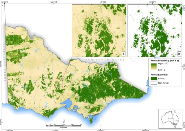
Figure 3-3 Implemented Random Forests model forest probability map (a) inset forest probability map (0– 100); (b) final forest classification, based on a binary threshold. ... 39

Figure 3-4 Random Forests predictor variable importance measures. ... 42

Figure 4-1 Effect of binary class imbalance on overall classification accuracy ... 64

Figure 4-2 Effect of binary class imbalance on mean margin ... 65

Figure 4-3 Binary classification unsupervised margin cumulative frequency distribution curve, comparing correctly and misclassified instance confidence, for optimal and critical training sizes. ... 66

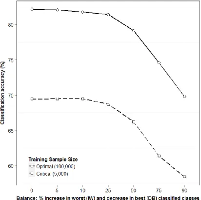
Figure 4-4 Effect of multiclass imbalance on overall multiclass classification accuracy ... 67

Figure 4-5 Effect of multiclass imbalance on mean margin ... 68

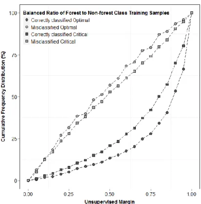
Figure 4-6 Unsupervised margin cumulative frequency distribution curves associated with correctly and misclassified instances, comparing balanced versus 50% increase/decrease open/closed ... 71

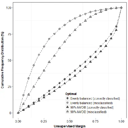
Figure 4-7 Unsupervised margin cumulative frequency distribution curves associated with correctly and misclassified instances, comparing balanced versus 90% increase/decrease open/closed ... 72

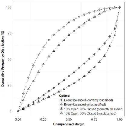
Figure 4-8 Unsupervised margin cumulative frequency distribution curves, comparing balanced and ratio-imbalanced (10 open: 90 closed) for optimal cases ... 73

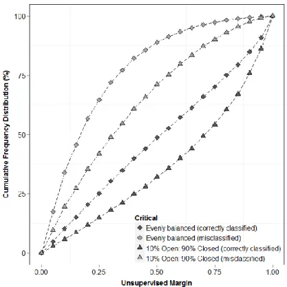
Figure 4-9 Unsupervised margin cumulative frequency distribution curves, comparing balanced and ratio-imbalanced (10 open: 90 closed) for critical cases ... 74

Figure 4-10 Effect of class mislabelling on binary classification overall accuracy ... 76

Figure 4-11 Effect of class mislabelling on binary classification mean margin ... 76

Figure 4-12 Effect of class mislabelling on multiclass classification overall accuracy ... 78

Figure 4-13 Effect of class mislabelling on multiclass classification mean margin ... 78

Figure 5-1 Study area map: Victorian Interim Biogeographic Regionalisation for Australia (IBRA Bioregions) and Aerial Photographic Interpretation (API) land cover maps. ... 90

Figure 5-2 Aerial photography examples of forest canopy cover used in the multiclass classification ( a) Woodland, 20-50% canopy cover; b) Open, 51-80% canopy cover; c) Closed, >80% canopy cover; d) Shrub (land cover dominated by woody vegetation shrub species, up to 2 m in height). Scale various around 1:25,000 ... 91

Figure 5-3 Flow chart illustrating training margins experiment (2) ... 93

Figure 5-4 Flow chart illustrating minimum node size experiment (3) ... 94

Figure 5-5 Ensemble and mean base classifier accuracies, mean margin and KW diversity plotted against mtry ... 96

Figure 5-6 Mean tree accuracy as a function of training set size by lowest and highest unsupervised margins, and random sampling ... 97

Figure 5-7 Ensemble accuracy as a function of training set size by lowest and highest unsupervised margins, and random sampling ... 98

(12)

xii

Figure 5-8 Ensemble KW diversity as a function of training set size by lowest and highest unsupervised margins, and random sampling ... 99 Figure 5-9 Ensemble accuracy for the open canopy class as a function of training set size by lowest and highest unsupervised margins, and random sampling ... 102 Figure 5-10 Ensemble accuracy for the closed canopy class as a function of training set size by lowest and highest unsupervised margins, and random sampling ... 102 Figure 5-11 Proportion of training samples by class and lowest unsupervised margins by percentile ... 103 Figure 5-12 Ensemble and mean base classifier accuracies and KW diversity as a function of minimum node size ... 104 Figure 6-1 Study areas map ... 110 Figure 6-2 Scatter plot showing curve linear trend between Number of Forest Patches and training data sampling margin percentile (Naringal) ... 118 Figure 6-3 Scatter plot showing curve linear trend between Edge Density and training data sampling margin percentile (Naringal) ... 118 Figure 6-4 Scatter plot showing curve linear trend between overall model accuracy and training data sampling margin percentile... 119 Figure 6-5 Scatter plot showing no significant relationship between Total area of forest and training data sampling margin percentile (Naringal) ... 120 Figure 6-6 Naringal forest extent map from classification training data sampled from the 40th percentile margin values ... 121 Figure 6-7 Naringal forest extent map from classification training data sampled from the 90th percentile margin values ... 121 Figure 6-8 Scatter plot showing curve linear relationship between the number the forest patches and training data sampling margin percentile (Newstead). ... 123 Figure 6-9 Newstead forest extent map from classification training data sampled from the 90th percentile margin values ... 124

(13)

xiii

List of Tables

Table 2-1 Victorian Forest Monitoring Program sample points by stratum, adapted from (Haywood et al.,

2016, 2017) ... 19

Table 3-1 Random Forests (RF) predictor variables ... 36

Table 3-2 Random Forests accuracy assessment. CI, confidence interval; OOB, out-of-bag. ... 40

Table 4-1 Optimal and critical training and test set sizes used for binary and multiclass experiments ... 55

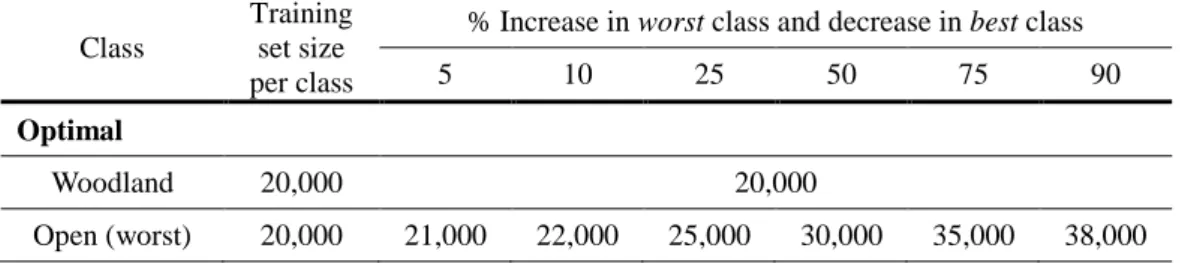
Table 4-2 Training set sizes for each class for multiclass imbalance (experiments 2 and 3) ... 56

Table 4-3 RF model performance results for binary classification imbalance (experiment 1) ... 63

Table 4-4 Binary imbalance confusion matrices and margin-weighted confusion matrices for evenly balanced and imbalanced training data in optimal and critical cases ... 63

Table 4-5 RF model performance results for optimal and critical multiclass classification imbalance experiments ... 68

Table 4-6 Multiclass imbalance confusion matrices and margin-weighted confusion matrices for optimal case (balanced and 50% imbalanced) ... 70

Table 4-7 RF model performance results for optimal and critical binary class mislabelling experiments ... 75

Table 4-8 RF model performance results for optimal and critical size multiclass class mislabelling experiments ... 79

Table 4-9 Multiclass mislabelling confusion matrices and margin weighted confusion matrices for optimal case ... 79

Table 4-10 Multiclass mislabelling confusion matrices and margin weighted confusion matrices for critical case ... 80

Table 5-1 Mean tree, ensemble accuracies (%) and Kappa statistic results for the number of predictor variables experiment ... 95

Table 5-2 Mean tree and ensemble accuracies (%), and Kappa statistic results for the training margin experiments ... 99

Table 5-3 Mean tree and ensemble accuracies (%) and Kappa statistic results for the minimum node size experiment ... 104

Table 6-1 Description of Landscape Pattern Indices (LPIs) ... 113

Table 6-2 Nature of the trend between margin-based training selection (40th to 90th percentile and random sampling) and LPIs for the Naringal Study area. Curve Linear (CL), Linear (L) or Not-significant (NS). 116 Table 6-3 Nature of the trend between margin-based training selection (40th to 90th percentiles and random sampling) and LPIs for the Newstead Study area. Curve Linear (CL), Linear (L) or Not-significant (NS). ... 116

Table 6-4 Nature of the trend between mislabeled training data (from 0% up to 30%) and LPIs for the Naringal Study area. Curve Linear (CL), Linear (L) or Not-significant (NS). ... 124

Table 6-5 Nature of the trend between mislabeled training data (from 0% up to 30%) and LPIs for the Newstead Study area. Curve Linear (CL), Linear (L) or Not-significant (NS). ... 125

(14)

1

(15)

2

1.1. Background: Large area land cover mapping

Timely and accurate large area land cover maps provide critical information to meet a range of environmental, social and economic needs. Such maps are essential inputs to a range of scientific applications, a source of input parameters for models and provide a basis of policy analysis (Wulder et al., 2008). Maps at a range of global, regional, national and sub-national scales, which characterise land cover and support land cover change assessment, support the needs of natural resource managers, scientists, policy makers and researchers (Vogelmann et al., 2004; Ståhl et al., 2016). The applications of such maps include assessment of global carbon budgets and climate modelling, assessing food security (Liu et al., 2008), predicting fire behaviour and hydrological modelling. Large area mapping products provide critical inventory data and information for understanding environmental processes and for effective natural resource management, land use planning and decision making (Lowry et al., 2007).

Satellite-based (remote sensing) earth observation has been recognised as an essential technology for large area, contiguous land cover mapping, which allows for frequent re-measurement for monitoring (DeFries and Townshend, 1994; Boyd and Danson, 2005; Hansen and Loveland, 2012; Chen et al., 2015). Remote sensing derived vegetation and forest maps (and forest cover change products) in particular, are important for understanding the spatial configuration and fragmentation of forest cover (Riitters et al., 2012), modelling forest productivity (Tramontana et al., 2015), invasive species and forest health (Coops et al., 2010) and locating priority areas for biodiversity conservation.

Remote sensing derived forest cover maps and monitoring systems are an important part of many national and regional forest inventory programs - used as a surrogate for field-based observations, to improve the precision of statistical estimates derived from field (plot) measurements and for creating spatially explicit forest cover maps (Deppe, 1998; McRoberts et al., 2005; McRoberts and Tomppo, 2007; Tomppo et al., 2010; Haywood et al., 2016). Forest extent is an indicator under the Montreal Process' seven criteria used to characterise sustainable forest management (Howell et

(16)

3

al., 2008) to which twelve countries are signatories, together representing about 60 per cent of the world's forests and 90 per cent of the world's temperate and boreal forests (Montréal Process Working Group, 2015).

1.2. Remote sensing for large area land cover

classification

Remote sensing classification - the transformation of image data into thematic map products has been a fundamental aspect of remote sensing since multi-spectral imagery first became available in the early 1970s (Wilkinson, 2005). Supervised classification in particular, is one of the most common forms of analysis undertaken with remote sensing data (Foody and Mathur, 2004). Supervised remote sensing image classification is broadly defined as the guided categorisation of pixels in an image (or remotely sensed data), to generate a particular set of labels of land cover themes (Lillesand and Kiefer, 1994). A review of image classification methods by Lu & Weng (2007), describes the complexity of this classification process, which requires many factors to be considered. These range from the determination of a suitable classification system, the selection of suitable training samples and image processing feature extraction, to post classification processing and accuracy assessment.

A review of remote sensing classification experiments by Wilkinson (2005), identified advances in three main areas of satellite image classification:

1. The development of particular components of classification algorithms - including training strategies;

2. Augmentation of classification algorithms through novel systems-level approaches;

3. The use of multiple types of ancillary data (including numerical and categorical data).

This fifteen year review (published in 2005) however, found as a whole, no significant upward trend in classification results across the hundreds of experiments reviewed (Wilkinson, 2005).

(17)

4

1.3. Machine Learning for remote sensing land cover

classification

Machine learning (ML) techniques – the advanced application of statistics to learning for identifying patterns in data and then making predictions from those patterns – have been used in a variety of science and engineering problems for nearly twenty years (Lary et al., 2016) and over the past decade have become increasingly popular techniques for remote sensing classification (e.g. Foody and Cutler, 2006; Foody et al., 2016; Ghimire et al., 2012; Graves et al., 2016; Rodriguez-Galiano et al., 2012; Rogan et al., 2008). Despite criticism directed at many ML techniques, considered 'black-boxes' which are unable to generate practical prediction equations (Lary et al., 2016), ML algorithms have proved to be more accurate and efficient techniques over traditional parametric approaches, particularly when dealing with large volumes of data across complex measurement spaces (Foody et al., 1995; Rogan et al., 2008). Unlike more traditional parametric classifiers, non-parametric ML algorithms make no assumptions as to the frequency distribution of input data. ML techniques do require prior knowledge about the nature of the relationships between the data (Lary et al., 2016). Traditional parametric techniques (such as Maximum Likelihood Classification) assume a normal distribution of data and as such, are limited in their application to multi-modal input data (Belgiu and Drăguţ, 2016). With respect to remote sensing data, which rarely have normal distributions, simple classifiers are also constrained in their application to dealing with the complex interactions between scene complexity, scale and aggregation (Marceau et al., 1994). Indeed, the application of traditional remote sensing classifiers are limited in heterogeneous landscapes which are characterised by land cover classes which are difficult to discriminate because of both low inter-class separability, as well as high intra-class variability (Ghimire et al., 2012). Other challenges include the complexity of measurement space and error and variability in calibration (reference) data (DeFries and Cheung-Wai Chan, 2000). Moisture, elevation and temperature (environmental) gradients and topographic heterogeneity also present challenges for image classification (Ghimire et al., 2012).

ML algorithms applied in remote sensing classification include Artificial Neural Network (ANN) (Foody and Arora, 1997; Yuan et al., 2009), deep learning neural

(18)

5

networks (Yu et al., 2017), Adaboost (Chan and Paelinckx, 2008; Haywood and Stone, 2011), Classification and Regression Tree (CART) (Lawrence and Wright, 2001). In recent years however, Support Vector Machines (SVM) and Random forests (RF) have stood out as the most popular ML classification algorithms used in the field of remote sensing. A Scopus database search across title, abstract and keywords "SVM" AND "Remote sensing" returned the highest number of publications, with an yearly average of 142 between 2010 and 2015. Over the same period, a search of "Random forests" AND "remote sensing" showed the highest annual increase in publications in remote sensing, with an annual average increase of 33% (compared to 27% for SVM). Moreover, across all fields (i.e. constraining the search terms to the algorithm name only), since 2010, the number of publications based on the search "Random forests" have increased on average 22% each year.

1.4. Random forests

Random forests (RF) (Breiman, 2001) is an ensemble machine learning technique that combines a collection of decision trees (created using random bootstrap samples of training data), and determines an output class through modal vote (classification) or mean prediction (regression) of the individual trees. Building on research by Amit & Geman (1997) and Ho (1998), Breiman (2001) developed Random forests, defining the classifier as consisting of a collection (or ensemble) of tree structured classifiers

{ℎ(𝒙, Θ𝑘),𝑘 = 1, … }

where Θ_𝑘 are independent identically distributed random vectors and each tree casts a unit vote for the most popular class at input.

Individual decision trees in a random forest ensemble are constructed by partitioning a subset training data (bagging sample) at each decision tree node, into increasingly homogeneous subsets, using randomly drawn predictor variables. The node-splitting predictor variable selected from the variable subset is one which results in the greatest increase in training data purity (variance or Gini) before and after the tree node split (Cutler et al., 2007). Purity here is defined as the relative homogeneity of training data in each sub-node after node splitting. This decision tree construction continues until there are no further gains in training data purity. Two key model

(19)

6

parameters need to be defined in training the random forest classifier (following notation in the randomForest library (Liaw and Wiener, 2002) available in statistical software package R (R Core Team, 2013).

1. The number of trees generated in the random forest ensemble (ntree)

2. The number of randomly selected predictor (or input) variables used at each decision tree split (mtry) - of this predictor variable subset, that which forms the best split is selected.

Figure 1-1 and Figure 1-2 illustrate the training and classification phases of the random forest classifier.

(20)

7

Figure 1-1 Random forest classifier training phase, adapted from Parnell et al. (2011)

Figure 1-2 Random forest classifier classification phase, adapted from (Nguyen et al., 2013)

Advantages of RF over other machine learning and traditional classifiers have been widely cited in the literature. Chiefly among its attributes are the excellent classification results, efficiency and processing speed (Pal, 2005; Du et al., 2015a; Chutia et al., 2016). Compared to other ML algorithms (such as Boosting and

(21)

8

Support Vector Machine), RF does not require a great deal of parameter adjustment and fine-tuning, with default parameterization often leading to excellent performance (Breiman, 2001; Svetnik et al., 2003; Statnikov et al., 2008) - this makes RF accessible, with good ease of use. Other cited advantages that demonstrate its performance and versatility include its applicability to both binary and multiclass prediction problems (Huang and Boutros, 2016); its handling of thousands of input variables (including a mixture of both categorical and continuous data), and providing estimates of their relative importance in the classification process; its ability to handle noisy observation data and outliers, in a complex measurement space and small training data relative to the study area size (DeFries and Cheung-Wai Chan, 2000; Rogan et al., 2008; Rodriguez-Galiano et al., 2012; Pelletier et al., 2017) and its ability to characterize complex variable interactions (Cutler et al., 2007). RF also demonstrates good predictive performance in applications with more variables than sample data (Huang and Boutros, 2016) and has been argued to not overfit (Peters et al., 2009). The RF algorithm grows an ensemble (forest) of decision trees which have high variance and low bias (Belgiu and Drăguţ, 2016).

The RF algorithm can handle diverse multisource remote sensing and geographic data (e.g. soil and terrain variables), making it well-suited to land cover classification (Corcoran et al., 2013; Inglada et al., 2017). Coupled with another of its advantages – the ability to produce variable importance measures, which aid interpretation of the classification model – RF can be used to evaluate the contribution and influence of data sources, for both optimising the classifier and interpreting results (which is typically more challenging in ensemble classification compared to an individual classification tree (Strobl et al., 2007).

1.5. RF classification reference data

The RF classifier has been shown to perform better with large numbers of training samples (Deng and Wu, 2013; Du et al., 2015b). Moreover, van der Ploeg et al. (2014) compared the performance of different machine learning techniques (including SVM and RF) for binary problem solving in relation to the effective sample size (or 'data hungriness'), and concluded that far more events per variable (10 times as many in this study) were needed to achieve stable model performance

(22)

9

(Area Under Curve) compared to classical techniques such as linear regression. Indeed, in the context of this medical study, the authors proposed that such "modern modelling techniques should only be considered....if very large data sets with many events are available" (van der Ploeg et al., 2014). These findings are consistent with earlier research (Selker et al., 1995), which found ML algorithms' ultimate limitations were associated with a "data barrier" (the availability of the information in data).

In an experimental study using data from various application domains, Dietterich (2000) established that boosting is more accurate than bagging. Boosting approaches have been shown to reduce classification variance and bias (Gislason et al., 2006; Ghimire et al., 2012). However, they require large computational resources, overfit if there are insufficient training samples, and are sensitive to any outliers present in the training samples. Other studies have also highlighted the sensitivity of the RF classifier to spatial auto-correlation of training data (Colditz, 2015; Millard and Richardson, 2015), as well as the proportion of different classes within training samples (Dalponte et al., 2013) – highlighting the importance of reference data given its cost and resource requirements.

In the context of large area supervised land cover classification using Earth observation data, the generation of reference data (hereafter used to describe the combination of training and validation or test data) whether through ground-based or sampled from high spatial resolution imagery, is an expensive and time consuming process (Ghimire et al., 2012; Gomez et al., 2016) and the quality of reference data can substantially affect the quality of derived land cover maps (Foody et al., 2016). Indeed, labelling reference data samples is prone to error and can result in poor classification performance and bias (Bradley and Friedl, 1996; Pal and Mather, 2006). Moreover, where ground truth data is assumed to be accurate, but does in fact contain errors, the classification algorithm can be wrongly supposed to be the source of inaccuracy rather than the training data (Carlotto, 2009).

Three developments are facilitating the take up and ease-of-use of modern machine learning algorithms, such as RF, for large area land cover classification problems. 1. Access to cloud computing

(23)

10

Cloud computing - the practice of using a network of internet hosted, remotely accessed servers to store, manage and process data, provides significant opportunities to address the challenge of large scale data-intensive remote sensing applications (Sugumaran et al., 2015). Increasing spatial, temporal, spectral and radiometric remote sensing data resolutions, across a range of platforms, coupled with access to data processing algorithms, and rapidly increasing internet data access and speed, is a technological nexus - one that can be referred to as big data (Sugumaran et al. 2015). Kumar et al. (2013) defines the questions as no longer "how do we capture imagery?", but rather, "how do we handle the immense volume of imagery we already have and to which we're adding every day?".

Amazon Web Services (a subsidiary of Amazon.com) provides a suite of cloud-computing, storage and analytics services in 13 regions across the world, from 2015 made publically available the entire archive of Landsat 8 scenes. Machine Learning AWS also provides tools to build machine learning models, including data analysis, training and evaluation. Google Earth Engine is a cloud-computing platform for processing satellite imagery and other earth observation data. GEE contains over 200 public datasets, over 5 million images and more than 5 petabytes of data. GEE's suite of tools include a suite of supervised classification algorithms (including Random forest, CART and SVM) and workflow for building, training, applying and assessing classification algorithms (Google Earth Engine Team, 2015).

2. Open Source software

Increasing ease of access to machine learning algorithms like RF via open-source software environments (including through cloud-computing services), allows users to access and readily automate classifiers through a set of adjustable parameters, which makes RF straightforward to apply for relatively inexperienced users (Qi et al., 2006). Several implementations of the RF classifier are now available, including the most popular randomForest (Liaw and Wiener, 2002) on the statistics package R (R Core Team, 2013), as well as implementations in Python, such as scikit learn Ensemble forest (scikit-learn developers, 2016) and through the Machine Learning Tool Kit (MILK) (Coelho, 2017) and Fast random forest in the WEKA Environment.

(24)

11

Launched in July 1972, Landsat 1 became the first global satellite earth observing mission (Belward and Skøien, 2015). The number of near polar orbiting operational earth observing satellite missions grew rapidly after 1972, to eight in August 1982, twenty a decade later, thirty-nine by August 2002 and eighty-three by 2012. Figure 1-3 (Belward and Skøien, 2015) shows the number of satellites operating by year and illustrates the rapid increase overtime.

Figure 1-3 The number of near-polar orbiting, land imaging civilian satellites operational as of 1 August 1972 to 2013 (Belward and Skøien, 2015).

Commensurate with the increase in earth observing platforms has been the increase in available remote sensing data. A policy change in 2008 resulted in the all new and archived United States Geological Survey (USGS) held Landsat satellite image data becoming freely available to any user (Wulder et al., 2012). The significance of this policy change cannot be underestimated - as at June 30 2016, over 42 million Landsat scenes have been downloaded by users worldwide (U.S. Geological Survey, 2017). Open data policies, like the Landsat Data Policy (http://landsat.usgs.gov/ documents/Landsat_Data_Policy.pdf), have increased the practicality of combining multiple data from multiple sensors and support data assimilation approaches for generating information, which, unlike in the meteorological community, are under-represented in terrestrial remote sensing (Wulder et al., 2012). Wulder et al. (2012) contend that the decision to make Landsat data freely available supports the efforts of international earth observing organisations in encouraging open data standards.

(25)

12

The range of open-access satellite imagery extends to the European Space Agency's Sentinel program (including 10 metre multispectral data) and Synthetic Aperture Radar (European Space Agency, 2016); MODIS (Moderate Resolution Imaging Spectroradiometer) aboard the Terra and Aqua satellites, acquiring data across 36 spectral bands over the entire Earth's surface every 1-2 days (NASA, 2016). Together with Landsat 8, the Sentinel satellite constellations will provide potential for landscape-scale observation data every three to four days (Turner et al., 2015). The combination of Landsat 8 and two Sentinel satellite sensors (2A and 2B) offer a global median average revisit interval of 2.9 days and maximum revisit interval of 7 days (Li and Roy, 2017).

Low-cost and accessible cloud-computing infrastructure, the free availability of access versions of a range of popular ML classification algorithms, and open-access policies for moderate resolution multi-spectral remote sensing data and a range of other spatial data, are all factors which promote the uptake of ML classifiers and provide great opportunities for improving the accuracy, currency and quality of large area land cover maps for a range of applications.

1.6. Research aims and experimental setting

In the context of large area classification using multisource remote sensing and geospatial data, the primary aim of this research is to examine two of the proposed advantages for RF described in this introduction - the relative insensitivity to training data noise (mislabelling) and its ability to handle class imbalance. This research will also investigate the utility of ensemble learning (and associated margin theory) – in which multiple base classifiers are combined to reduce generalisation error in classification – to design more efficient classifiers, improve classification performance, to reduce reference data redundancy and design ensemble classification systems which use reference data more efficiently and effectively.

The experimental setting and data used in this research (introduced and described in detail in chapters 2 and 3) provides a unique real-world testing environment through which to explore and apply ML concepts – typically constrained to simulation-based studies in the field of information science – to a large area remote sensing problem, using reference data (stratified, unbiased and proportional to the study area) and an

(26)

13

environment which is both realistic and a representative testing environment to provide insights for classification problems applied in alternative geographic settings where greater reference data typically constraints apply.

1.7. Research Questions

Three research questions are explored in this thesis:

Question 1: How do training data characteristics of class imbalance and class mislabelling affect RF performance?

This question is explored through the application of margin theory, employed as a measure of confidence in classification results, to supplement traditional classification performance measures used in remote sensing classification.

Question 2: What is the relationship between ensemble diversity and classification performance?

This question seeks to examine the degree of influence that ensemble diversity has on classification performance, and how ensemble classifier diversity can be controlled to improve the efficiency and effectiveness of classification training data.

Question 3: What is the relationship between training data characteristics (used to

construct RF ensemble classification models) and Landscape Pattern Indices (LPIs) calculated from RF derived prediction maps?

This questions looks at the application of RF classification models to generate LPIs, and examines the sensitivity of these indices to training data characteristics and sampling based on the ensemble margin.

1.8. Thesis structure

This thesis is presented such that each chapter (with the exclusion of the introduction and synthesis) may be read independently. The research chapters match the published (or prepared for publication) versions, with changes only to formatting in order to maintain a consistent style through the thesis. Cited references are compiled into a single bibliography at the end of the thesis.

(27)

14

The thesis comprises seven chapters, of which four are research chapters (three of which have been published in peer-reviewed journals). There is no stand-alone literature review chapter, as these are included in the introduction sections of each research chapter.

Chapter 2 describes the experimental setting for this research - including the sampling framework for the reference (training and test) data used in classification experiments that follow. This chapter summarises the advantages and opportunities afforded by the experimental design to explore the key research questions introduced in Chapter 1. Chapter 3 evaluates the performance of the Random forest (RF) classifier applied across 7.2 million hectares of public land in Victoria, Australia. This chapter describes an open-source framework for deploying the RF classifier over large areas and processing significant volumes of multi-source remote sensing and ancillary spatial data.

Chapter 4 examines the effect of training data characteristics of class imbalance and mislabelling on the performance of Random forests. Through different experiments applied to binary and multiclass problems, this research chapter examines the sensitivity of RF classification performance to training class imbalance and training data mislabelling. Chapter 4 also introduces the ensemble margin, and derived metrics that can be used as ancillary measures of classification performance.

Chapter 5 explores the relationship between per-class and overall classification performance and the diversity of members in a RF ensemble classifier. This chapter brings together the understanding of the ensemble margin developed in Chapter 4, to look at ways to target particular training data samples to induce ensemble diversity and improve per-class and overall classification performance and efficiency.

Chapter 6 explores the application of the RF classifier for deriving landscape pattern indices from classification prediction maps and examines the sensitivity of these indices to training data characteristics and sampling based on the ensemble margin. Chapter 7 provide a synthesis of the research and discussing the research findings and their implications in the context of recent technology and data developments, which have increased the accessibility of advanced classification algorithms such as RF.

(28)

15

Chapter 2. Experimental Setting and

(29)

16

2.1. Experimental setting

The following chapter describes the experimental context for this research - including the study area and the sampling framework for the reference (training and test) data used in large area land cover classification experiments that follow. This chapter summarises the advantages and opportunities afforded by the experimental design to explore the key research questions introduced in Chapter 1.

2.2. Victorian Forest Monitoring Program

The reference data used in the research experiments described in chapters 3 through 6, is drawn from the Victorian Forest Monitoring Program (VFMP). The VFMP (Haywood et al., 2016; Haywood and Stone, 2017) is a strategic forest inventory established in the State of Victoria in south east Australia. The VFMP combines field measurement plots with remote sensing data across the State's public land forests, the information from which is used to assess Victoria’s progress towards achieving sustainable forest management objectives and targets (Haywood et al., 2016). The VFMP and other similar strategic forest inventories have been established in many jurisdictions around the world (e.g. in north America and Scandinavia) – historically with the primary objective of monitoring and assessing forest (i.e. timber) resources. More recently however, there has been a shift in public focus and awareness towards the essential role that forests also play in climate regulation, as a source of biological and genetic diversity, in the storage and maintenance of carbon cycles, and the provision of cultural, tourism and amenity values (Myers, 1996; Boyd and Danson, 2005). The increasing need for consistent data with which to make comparisons between land and forest management regimes or between different jurisdictions is also driving the need to establish and maintain forest data collection systems – which also support national and international forest policy and decision making.

2.3. Design-based sampling

The VFMP uses a design-based sampling framework (also known as a probability-based sampling design) - a classical approach to sampling (Cochran, 1977), for which the objective is to describe the characteristics of a real and explicitly defined population. Such sampling is necessary to address the impracticality of collecting

(30)

17

reference data for a census of an entire region (Stehman, 2000). In design-based frameworks, sampling locations are selected through probability sampling and statistical inference used to, for example, estimate a spatial mean, is based on sampling design (Brus, 2010). Design-based inference typically assumes a finite population of elements to which one or more fixed target quantities are linked (Ståhl et al., 2016). In contrast to design-based sampling, model-based sampling does not have requirements on a method for selecting sampling locations, and typically are selected by purposive (targeted) sampling, for instance on a centred grid (Brus, 2010). Model-based approaches, sometimes characterized as model dependent approaches (Hansen et al., 1983), use predictions based on models and ancillary variables to produce estimates (McRoberts, 2010).

Simple random sampling and systematic sampling are sampling approaches which provide a foundation for most probability or design-based sampling. The VFMP applies stratified random sampling for its design-based approach. In stratified random sampling, the total population is divided into mutually exclusive, non-overlapping strata, from which simple random samples are taken. Each potential sample unit can only be assigned to one stratum and all unit are included. Among the advantages of stratified random sampling include minimizing sample selection bias and reducing over and under-representation of certain population segments.

2.4. VFMP Sampling Design

The VFMP is a plot-based design made up of permanent observational units located on a state-wide grid (Haywood and Stone, 2017). The guiding principle of the VFMP design is the consistency of data collected through monitoring, whereby the same attributes are measured over space and time, with the same standards and in a statistically defensible manner and at an acceptable level of precision. For the VFMP, the desired stratum level target precision (standard error) is 12.5%. The VFMP's sampling framework has the following key elements (which are described in further detail below) (Haywood et al., 2017).

(31)

18

2. Stratification: Two-way stratification of the target population with each stratum adequately sampled for statistical reliability through variable sampling intensity.

3. Plot design: comprising two components, a) ground-based - from which a range of direct measurements of forest structure and composition are taken, and b) a remotely sensed photo-plot

2.5. Target population

The target population (study area, or sampling frame) comprises 7.1 million hectares of public land, covering about one third of the state of Victoria, in south East Australia. This includes about 3.9 million hectares of mostly forested parks and conservation reserves – managed primarily for ecosystem and biodiversity conservation, as well as tourism, recreation and cultural and historic values. State forests cover about a further 3.1 million hectares – land management in State forests include the water catchments and water supply, flora and fauna conservation, as well as the provision of timber (The State of Victoria Department of Environment and Primary Industry, 2013). The target population is assumed to consist of an infinite number of points within the public land estate. Chapter 3 includes a more detailed description of the study area climatologically and environmental and topographic characteristics.

2.6. Sampling Stratification

The target population was stratified with respect to two factors, bioregion and tenure. Firstly, the target population was stratified into 11 IBRA (Interim Biogeographic Regionalisation for Australia) Bioregions – these are large and geographically distinct areas of land which share common geology, landform, climatic and ecological characteristics (Cummings and Hardy, 2000). The target population was further stratified into the two major public land tenure (Parks and Reserves, including national, state, and regional parks, and State forest (described above). Figure 2-1 shows the distribution of sampling plots (units) located across Victoria's major public land tenures. Figure 2-2 shows the sampling plots (units) and IBRA Bioregions (the primary stratification unit).

(32)

19

Within each stratum, sample units were placed at the intersections of a grid which utilised the VicGrid coordinate system (DSE, 2000) whose spacing varied between 2 km and 20 km and was selected to produce a per stratum sample size of approximately 30 samples. The target within-stratum sample size of 30 samples was based on the assumption of a coefficient of variation for a quantitative trait measured in the VFMP (such as biomass) of at least 70% and a stratum-level target precision (or standard error) of no more than 12.5% (Haywood et al., 2016). Within a geographically large stratum, sample points are more widely spaced to achieve the optimal and most resource efficient target number of sampling locations, compared to smaller strata. Table 2-1 shows the number and spacing of Victorian strategic forest inventory sample points by stratum. A more detailed description of the VFMP sampling design and its rationale can be found in Haywood et al. (2016). Unlike many other strategic forest inventories - which collect information about the state and dynamics of forests for management planning - the VFMP sampling (from field and remote sensing) deliberately extends to include all land covers types within the public land estate.

Table 2-1 Victorian Forest Monitoring Program sample points by stratum, adapted from (Haywood et al., 2016, 2017) IBRA Bioregion Parks and Reserves Grid spacing (km) State forest Grid spacing (km) Sample Units Australian Alps 36 10 53 8 Flinders 26 4 * - Murray-Darling Depression 39 20 28 10

Naracoorte Coastal Plain 42 4 42 4

NSW South Western Slopes 43 4 31 4

Riverina 69 6 8 4

South East Coastal Plain 27 8 25 4

South East Corner 39 10 44 12

South East Highlands 49 12 42 18

Victorian Midlands 35 10 38 8

Victorian Volcanic Plains 30 6 40 2

Total 435 351

(33)

20

Figure 2-1 Location of sampling units (plots) across Victoria's public land Forest Monitoring Program

(34)

21

2.7. Sampling

The plot design of each sample point comprises two main components – a multi-staged field-plot and an aerial photoplot. At the field-plot level, 215 variables are measured and assessed, within a 0.04 ha circular plot and soil and vegetation quadrats. These variables include physical and biotic characteristics (such as slope, aspect, topographic position and site disturbance), as well as tree measurements (e.g. species, diameter at breast height over bark, canopy health and cover), coarse woody debris, understory vegetation and groundcover attributes and soil. A detailed description of the field-plot inventory method and attributes measured is available in Haywood et al. (2016).

Above each field-plot point, 2 km x 2 km photoplot sampling units provide the primary source of land cover information for the VFMP inventory and the source of reference data used in the research experiments described in the following chapters. Digital high resolution (30 cm and 50 cm pixels) colour (RGB and Near Infrared) aerial photographs acquired over the period 2006 to 2010 were used to map landcover, following a classification system comprising broad forest type, height and canopy cover classes (Mellor and Haywood, 2010). A detailed description of the land cover mapping method applied to VFMP photoplots and used as the source of reference data in this study, is included in chapter 2 and documented in Farmer et al. (2013).

Figure 2-3 illustrates the primary sampling components of the VFMP ground plot, together with an example land cover photoplot map (above).

(35)

22

Figure 2-3 Primary components (field plot and aerial photoplot) of the VFMP sampling unit

2.8. Summary

The design-based statistical sampling framework of the VFMP and the nature of the photoplot sampling units from which reference data is collected, afford several advantages which provide a unique opportunity to explore how training data characteristics affect RF performance in this research. For example, the spread of sampling units is comprehensive and their geographic coverage extensive. The

(36)

23

systematic and stratified sampling framework helps ensure that sampling is balanced, unbiased and addresses heterogeneity characteristics of the large and diverse study area. Furthermore, the training data generated at sampling units is temporally consistent.

These training data sampling characteristics are not typical - particularly in large regions or jurisdictions in which areas are inaccessible or suitable high resolution data is scarce. Research findings from this exemplar reference dataset from a real-world experimental environment, might be used to design and parameterise more efficient ML classifiers in other jurisdictions, making more efficient and effective use of training data, which may of poorer quality (e.g. less geographic or class coverage, noisy and mislabelled and collected with temporal variability).

(37)

24

Chapter 3. The Performance of

Random Forests in an

Operational Setting for

Large Area Sclerophyll

Forest Classification

Based on the peer-reviewed published article:

Mellor, A., Haywood, A., Stone, C. and Jones, S., 2013. The performance of

random forests in an operational setting for large area sclerophyll forest classification. Remote Sensing, 5(6), pp.2838-2856.

(38)

25

3.1. Introduction

Forest extent is a measure commonly assessed in national forest inventories (NFI) (McRoberts, 2010) and, under the Montreal process (Howell et al., 2008), is a specific indicator used for monitoring and reporting sustainable forest management. For natural resource management agencies, current and accurate forest area estimates are critical for effective environmental monitoring. While ground-based (field plot) forest inventories can provide accurate and unbiased forest area estimates, spatially explicit remote sensing-derived forest extent maps can be used to assess the spatial configuration of forest at the landscape scale and used in combination with a high resolution sample (two-staged sampling) to improve forest area estimates (Deppe, 1998).

In Australia, under the Australian National Forest Inventory, forest is defined as “A land area, incorporating all living and non-living components, dominated by trees having usually a single stem and a mature or potentially mature stand height exceeding two metres and with existing or potential crown cover of overstory strata about equal to or greater than 20 percent. This definition includes native forests and plantations and areas of trees that are sometimes described as woodlands” (Department of Agriculture Fisheries and Forestry, 2012). The structural components in this definition encompass a wide range of forest types, from open low sparse canopy woodland to tall dense canopy forests (as illustrated by Figure 3-1, (Australian Surveying and Land Information Group, 1990)).

In Australia (and the state of Victoria, in particular), dry, damp and wet sclerophyll forests and woodlands comprise many of the forested ecosystems. The canopies in these ecosystems are dominated by eucalypt species and are characteristically open with irregular (asymmetrical) crown configurations and low foliage density (Jenkins and Coops, 2011). Canopy foliage is often clumped, leaves tend to concentrate around crown perimeters (Jacobs, 1955) and exhibit an erectophile (vertical) leaf angle distribution. In Victoria, as in much of Australia’s forests, there is a high diversity of forest development phases, vertical and horizontal forest structures, topography and soil types (Behn et al., 2001), as well as dynamic phenological processes in understory vegetation (Bhandari, 2011).

(39)

26

These characteristics pose a number of challenges to the use of remote sensing in these environments for classifying and mapping forests. The mid- and under-story components, shadows and background soils all exhibit a strong influence on spectral reflectance characteristics. From a synoptic perspective, forest cover in Victoria can appear indistinguishable from shrub and other low and sparse woody vegetation species. Complexity and background noise in remote sensing signatures from open sclerophyll eucalypt forests is further intensified by the influence of dynamic understory elements and variation in forest structures (Jupp and Walker, 1997). The challenges and complexities associated with forest extent mapping across state and territories in Australia is evidenced by large differences and inconsistencies in forest extent maps and forest area estimates produced by state and federal government agencies and the variability in forest area estimates published in Australia’s national five-yearly State of the Forests reports (Montreal Process Implementation Group for Australia, 2008). The processing of large area remote sensing datasets poses a further challenge for state land management agencies.

Figure 3-1 Australian forest structural definitions (Australian Surveying and Land Information Group, 1990).

(40)

27

Random Forests (RF) (Breiman, 2001) offers a possible solution to address these large area forest classification challenges, universal across many of Australia’s forest ecosystems. Machine learning classifiers, such as RF, are increasingly being used for environmental mapping and modelling applications in fields, such as natural resource management and forestry (Main-Knorn et al., 2011; Clerici et al., 2012; Rodriguez-Galiano et al., 2012). RF is an ensemble decision tree classifier, which combines bootstrap sampling to construct many individual decision trees, from which a final class assignment is determined (Breiman, 2001).

RF can be used to learn complex non-linear relationships, such as those present in variable vertical forest structure and the association of overstory to understorey forest vegetation. RF has been demonstrated to be very effective for accurate land cover mapping across complex and heterogeneous landscapes and to be relatively insensitive to noise (Rodriguez-Galiano et al., 2012), making it suitable for application in complex and dynamic forest environments. As RF does not require normally distributed model training data, its application is appropriate for areas where species distributions of ecological communities follow non-linear patterns across the landscape (Austin and Meyers, 1996) and where complex terrain effects data normality (Khalyani et al., 2012). Other reported benefits of RF include its relative insensitivity to outliers (Breiman, 2001; Cutler et al., 2007), common characteristics of open canopies across large areas of dynamic and highly variable forest ecosystems. Furthermore, the RF classifier runs efficiently on large datasets (Rodriguez-Galiano et al., 2012), making it suitable for regional-scale mapping, comprising millions of hectares.

As only a random subset of variable data is used to construct each decision tree in a random forest classifier ensemble, correlation between decision trees is reduced, thereby improving predictive power and classification accuracy, whilst decreasing the computational complexity of the algorithm. As has been demonstrated in recent studies (Fahsi et al., 2000; Joy et al., 2003; Gislason et al., 2006; Sesnie et al., 2008), RF can incorporate multiple-sources of remote sensing data with ancillary continuous and categorical biophysical spatial data to improve classification performance and discriminate between forest and non-forest.

(41)

28

Moderate resolution multi-spectral imagery, such as Landsat Thematic Mapper (TM)/Enhanced Thematic Mapper (ETM+) has been commonly applied for estimating forest cover (Green and Sussman, 1990; Boyd and Danson, 2005), discrimination of some forest types (Lu et al., 2003), forest cover change detection (Tucker and Townshend, 2000; Rogan, 2002) and for model-based forest area estimation (McRoberts, 2010). Because of the challenges described above, limitations arise in classifying forest extent where different forest structures and composition and land cover types can appear spectrally alike using traditional remote sensing data analysis techniques. Improved forest classification accuracy and forest area estimates have been achieved for large areas using multi-temporal imagery, e.g., MODIS (Wulder et al., 2010; Maselli, 2011). The high temporal resolution of the MODIS sensor can provide valuable information about the phenological variability of different land covers and, as such, help address the challenge of forest canopy-to-understory discrimination in the type of open canopy forest environments described above. In the context of open-canopy forest extent classification, textural information (spatial variation data derived from optical imagery) can provide additional information to a RF classifier, by differentiating vegetation that appears spectrally similar when integrated into a remote sensing image pixel, but whose spatial patterns differ (Culbert et al., 2009). Recent studies have used satellite image-derived texture indices to improve forest stand classification (Coburn and Roberts, 2004), biomass and carbon estimation (Lu, 2005; Proisy et al., 2007; Eckert, 2012) and forest structure derivation (Kayitakire et al., 2006). In a large heterogeneous landscape RF classification study, Rodríguez-Galiano et al. (2011), increased overall accuracy by 8% (and Kappa by 9%) by including textural information.

The conditional relationships between forest vegetation and biophysical factors can also be used to further improve forest/non-forest discrimination. Species-environment relationships are central to predictive geographical modelling (Guisan and Zimmermann, 2000). Topographic variables (e.g., elevation, slope and aspect) used in combination with spectral data have been demonstrated to enhance forest, habitat and vegetation classification (Fahsi et al., 2000; Joy et al., 2003; Gislason et al., 2006; Sesnie et al., 2008). Bioclimatic maps (e.g., temperature, precipitation) are an additional source of commonly used ancillary classification data.