Active Bayesian Assessment for Black-Box Classifiers

(1)

Title

Active Bayesian Assessment for Black-Box Classifiers

Permalink

https://escholarship.org/uc/item/30v539zh

Journal

CoRR, abs/2002.06532

Authors

Ji, Disi

IV, Robert L Logan

Smyth, Padhraic

et al.

Publication Date

2020

License

https://creativecommons.org/licenses/by/4.0/ 4.0

Peer reviewed

(2)

Active Bayesian Assessment for Black-Box Classifiers

Disi Ji [email protected]

Department of Computer Science University of California, Irvine

Robert Logan [email protected]

Padhraic Smyth [email protected]

Mark Steyvers [email protected]

Department of Cognitive Science University of California, Irvine

Abstract

Recent advances in machine learning have led to increased deployment of black-box classifiers across a wide variety of applications. In many such situations there is a crucial need to assess the performance of these pre-trained models, for instance to ensure sufficient predictive accuracy, or that class probabilities are well-calibrated. Furthermore, since labeled data may be scarce or costly to collect, it is desirable for such assessment be performed in an efficient manner. In this paper, we introduce a Bayesian approach for model assessment that satisfies these desiderata. We develop inference strategies to quantify uncertainty for common assessment metrics (accuracy, misclassification cost, expected calibration error), and propose a framework for active assessment using this uncertainty to guide efficient selection of instances for labeling. We illustrate the benefits of our approach in experiments assessing the performance of modern neural classifiers (e.g., ResNet and BERT) on several standard image and text classification datasets.

1. Introduction

Complex machine learning models, particularly deep learning models, are now being applied to a variety of practical prediction problems ranging from diagnosis of medical images (Kermany et al., 2018) to autonomous driving (Du et al., 2017). As a result, software systems with embedded machine learning components are becoming increasingly common. Many of these models will be black boxes from the perspective of downstream users, such as models developed remotely by commercial entities and hosted as a service in the cloud (Yao et al., 2017). For a variety of reasons (legal, economic, competitive), users will often have no direct access to the detailed workings of the model, how the model was trained, or the training data.

In this context it is increasingly important for the user of a model to have accurate and robust assessments of the quality of a model’s predictions. However, as an example, “self-confidence" estimates provided by machine learning predictors can often be quite unreliable and miscalibrated (Zadrozny and Elkan, 2002; Kull et al., 2017; Ovadia et al., 2019). In particular, complex models such as deep networks with high-dimensional inputs (e.g., images and text) can be significantly

(3)

0.5

1.0 lizard

otter

seal

shrew

bear

boy

woman

couch

shark

baby

...

bicycle

castle

pickup truck

skunk

apple

palm tree

wardrobe

motorcycle

sunflower

keyboard

CIFAR-100 Labels

Accuracy

0.0

0.2 ECE

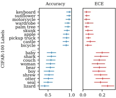
Figure 1: Mean posterior estimates and 95% credible intervals for the classwise accuracy and expected calibration error (ECE) of a ResNet-110 image classifier on the CIFAR-100 test set, using our Bayesian assessment framework. For further details see Section 3.

overconfident in practice (Gal and Ghahramani, 2016; Guo et al., 2017; Lakshminarayanan et al., 2017). Furthermore, test set performance metrics from train-test splits might not be an accurate reflection of downstream performance due to factors such as label and distribution shift (e.g., Lipton et al. (2018); Hendrycks and Gimpel (2017); Ovadia et al. (2019) and/or implicit optimistic bias (Recht et al., 2019).

Thus, downstream users of black-box predictors will need the capability to carry out assessment separately and independently from the training and evaluation procedures used when fitting the model. This assessment could for example be conducted by organizations not involved in training the model, in a manner similar to the assessments of commercial products carried out by regulatory agencies. Additional motivations for independent assessment include legal requirements that may mandate independent assessment of models, the need to build trust on the part of a human consumer of model predictions, or situations where the predictor is being deployed in an environment with a different distribution over inputs and outputs compared to the environment the model was trained on.

In this paper we develop a Bayesian framework for performing this assessment that requires no internal access to the model being evaluated, only its output probabilities. We focus on classification models in particular, although the ideas are broadly applicable to prediction models in general. Figure 1 provides an illustrative example applying our approach to assess performance of a ResNet classifier on the CIFAR-100 dataset, with detailed assessments of the classwise accuracy and calibration properties, along with posterior credible intervals measuring how certain we are in our assessment given the data available.

Assessment of model properties such as accuracy and calibration requires labeled data. In real-world deployment scenarios, this data is likely to be scarce and costly to collect, e.g., consider a pre-trained classification model being deployed in a diagnostic imaging context in a particular hospital. With this in mind we also develop a framework for active assessment of black-box classifiers,

(4)

Mode Size Classes Model CIFAR-100 Image 10K 100 ResNet-110

ImageNet Image 50K 1000 ResNet-152 SVHN Image 100K 10 ResNet-152 20 Newsgroups Text 7.5K 20 BERTBASE

DBpedia Text 70K 14 BERTBASE

Table 1: Assessment datasets and models used in our experiments. Size refers to the maximum number of labeled instances available for assessment.

using techniques from active learning to efficiently select instances to label so that model deficiencies such as low accuracy, or high cost mistakes can be quickly identified.

In summary, our primary contributions are:

• We propose a general framework for black-box classifier assessment, using a Bayesian approach that is applicable to a range of performance-related metrics.

• We illustrate the utility of the framework via Bayesian inference with posterior uncertainty for quantities such as classwise accuracy, expected calibration error (ECE), and reliability diagrams.

• We develop a new framework called active assessmentand demonstrate how this framework can be used to identify extreme classes in an online label-efficient manner with significant gains over traditional random sampling methods.

2. Preliminaries

2.1 Notation

We consider classification problems with a feature vector xand a class labely ∈ {1, . . . , K}, e.g., classifying image pixelsxinto one ofKclasses. We assume access to a trained prediction model M

that makes predictions ofygiven a feature vectorx. In particular we assume that the model produces numerical scores per class, reflecting its confidence, typically in the form of a set of estimates of class-conditional probabilitiespM(y=k|x), k= 1, . . . , K. Such probability estimates can be obtained from a logistic classifier, from the softmax output layer of a neural network, from averages over leaf nodes in tree-based models, and so on. A notational aside: for probabilities that are being generated by the model we use subscriptM, e.g.,pM(y=k|x). When we refer to the actual true probability with respect to the underlying true distribution p(x, y)we drop the subscript, e.g., when using terms likep(y=k|x)andp(x)in computing expectations.

Under 0-1 classification loss,yˆ= arg maxkpM(y=k|x)will be the classifier’s label prediction for a particular inputx. We can defines(x) =pM(y= ˆy|x)as thescoreof a model, as a function ofx, i.e., the class probability that the model produces for its predicted classyˆ∈ {1, . . . , K} given input

x. This is sometimes also referred to as a model’sconfidencein its prediction and can be viewed a model’s own estimate of its accuracy when it predictsyˆgivenx. The model’s scores in general need not be perfectly calibrated, i.e., they need not match the true probabilitiesp(y= ˆy|x).

2.2 Datasets and Classification Models

Assessment Datasets We assess performance characteristics of neural models on several standard image and text classification datasets. The image datasets we use are: CIFAR-100 (Krizhevsky and Hinton, 2009), SVHN (Netzer et al., 2011) and ImageNet (Russakovsky et al., 2015). The text datasets we use are: 20 Newsgroups (Lang, 1995) and DBpedia (Zhang et al., 2015). Detailed

(5)

statistics are provided in Table 1. The assessment datasets are based on standard test sets used for each dataset in the literature.

Prediction Models For image classification we use ResNet (He et al., 2016) architectures with either 110 layers (CIFAR-100) or 152 layers (SVHN and ImageNet). For ImageNet we use the pretrained model provided by PyTorch, and for CIFAR and SVHN we use the pretrained model checkpoints provided at: https://github.com/bearpaw/pytorch-classification. For text clas-sification tasks we use fine-tuned BERTBASE (Devlin et al., 2019) models. These models were all trained on standard training sets in the literature, independent from the datasets used for assessment. To facilitate reproducing our results we provide all of the model predictions used in our experiments at: https://github.com/disiji/bayesian-blackbox.

3. Bayesian Assessment of Classification Metrics

We focus on the problem of assessing the performance of a model on data drawn from some unknown distribution p(x, y)representing the environment where the model is being used. This joint distribution in general need not necessarily be the same as the distribution that the model was trained on. We are interested in particular in the situation where the model is a black box, where we can observe the inputsxand the outputspM(y=k|x), but don’t have any other information about its inner workings (for example about any internal parameters of the model). Specifically, in this paper, rather than learning a model itself we want to learn about the characteristics of a fixed model that is making predictions in a particular environment.

A natural approach to assessing the performance of a black-box classifier is to adopt a Bayesian framework where we treat the metrics of interest (classification accuracy, calibration error) as unknown parameters that we estimate from (limited) labeled data drawn from a distributionp(x, y).

3.1 Assessing Classwise Accuracy

Beginning with classification accuracy, themarginal accuracyof a classification model is defined as

A(x) =p(y= ˆy|x). We also defineregional accuracyover local regions of the input space. For any

regionRin the input space, regional accuracy is the marginal probability that the predicted label matches with the true label, conditioned onx∈ R:

AR = Ep(x,y|x∈R)[A(x)]

=

Z

R

p(y= ˆy|x)p(x|x∈ R)dx. (1)

We will use this as one of our main assessment tools.

In particular, we will focus on assessment ofclasswise accuracy,ARk, k= 1, . . . , K, the expected accuracy of the model whenever it predicts classk. This corresponds to having the input region be the classifier’s decision regionRk={x|yˆ=k}. To estimate the classwise accuraciesARk from data, a standard approach would be to empirically approximate the integral above by samplingx, y pairs from the conditional distributionp(x, y|x∈ Rk). Equivalently,ARk can be modeled as an unknown Bernoulli parameterθk, with draws(x(i)_{, y}(i)_{), conditioned on}_x_{∈ R}_{k, leading to binary outcomes}

1(y(i)_{= ˆ}_y(i)₎_{∈ {}₀_,₁_}_{, with a frequency-based (maximum likelihood) estimate:} ˆ θk = 1 S S X i=1 1(y(i)= ˆy(i)). (2) It is natural to consider Bayesian estimation in this context, especially in situations where there is little labeled data available for assessment and/or where the number of regions K is large. In particular, we can put a Beta(αk, βk)prior onθk, model the draws1(y(i)= ˆy(i))with a binomial

(6)

0.0 0.5 1.0 0.0 0.5 1.0 Accuracy N=100 0.0 0.1 0.2 0.3 0.0 0.5 1.0 0.0 0.5 1.0 Accuracy N=1000 0.0 0.1 0.2 0.3 0.0 0.5 1.0 Score (Model Confidence) 0.0

0.5 1.0

Accuracy

All labeled data

0.0 0.1 0.2 0.3 ECE Frequentist Ground truth Bayesian 0 0.5 1.0 0 0.5 1.0 0 0.5 1.0

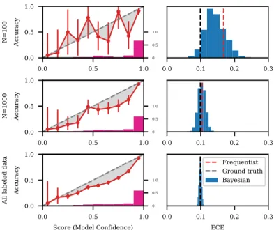
Figure 2: Bayesian reliability diagrams (left) and posterior densities for ECE (right) for CIFAR-100 as the amount of data used for estimation increases. Vertical lines in the right plots depict the ground truth ECE (black, evaluated with all available assessment data) and frequentist estimates (red).

likelihood, and produce Beta posteriors for each θk, k = 1, . . . , K. The Bayesian approach allows for uncertainty in our inferences about quantities such asθk =ARk as well as providing a basis for supporting techniques such as active selection of examples for labeling (discussed later in the paper). In situations where we have noa prioriinformation aboutθk we can use a weak uninformative prior

with αk =βk= 1; alternatively, we can use strong prior information (e.g., if the assessor believes the

performance metrics reported by the model-builder) when available.

102 103 104 #queries

0% 15% 30%

ECE estimation error

CIFAR-100 102 103 104 #queries 0% 50% 100% ImageNet 102 103 104 #queries 0% 75% 150% SVHN 102 103 104 #queries 0% 8% 16% 20 Newsgroups 102 103 104 #queries 0% 100% 200% DBpedia Bayesian Frequentist

Figure 3: Percentage error in estimating expected calibration error (ECE) as a function of dataset size, for Bayesian (red) and frequentist (blue) estimators, across five datasets.

3.2 Assessing Calibration Performance

We can also assess calibration-related metrics for a classifier in a Bayesian fashion using any of well-known various calibration metrics (Kumar et al., 2019; Nixon et al., 2019). Here we focus on expected calibration error (ECE) given that it is among the widely-used calibration metrics in the machine learning literature (e.g., Guo et al. (2017); Ovadia et al. (2019)). We use the standard ECE

(7)

binning procedure, with scores aggregated into equal-width bins, denoting theb-th bin or region as:

Rb={x|s(x)∈[(b−1)/B, b/B)}, (3)

whereb= 1, . . . , B(B= 10is often used in practice). Note that these are not the decision regions induced by the model that we discussed earlier but instead are a partition of the input space determined by the score of the predicted classs(x). The marginal ECE is defined as a weighted average of the absolute distance between the true accuracyθb and the average scoresb per bin:

ECE=

B

X

b=1

pb|θb−sb| (4)

where pb is the probability of a score lying in binb. The unknown accuracy of the model per bin is

θb, which can be viewed as a marginal accuracy over the regionRb in the input space corresponding tos(x)∈Binb, i.e., θb=

R

Rbp(y= ˆyM|x)p(x|x∈ Rb)dx.

To assess the marginal ECE (Eqn. 4), we put Beta priors over the θb’s,b= 1, . . . , B. Our default setting for the priors is a weak prior (α+β = 2) with the mean of the prior on the diagonal for each bin, i.e., we assumea priorithat the model is calibrated but allow the data to easily overwhelm the prior if there is evidence that the model is not well-calibrated. The posterior distribution over ECE is a weighted average of the absolute value ofB shifted Beta posterior distributions corresponding to the individualθb’s. The posterior is not available in closed form but Monte Carlo samples are straightforward to obtain.

As for accuracy, we can also model classwise ECE, ECEk =PB

b=1pb,k|θb,k−sb|, by modifying the model described above to use regions Rb,k ={x|yˆ=k, s(x)∈Binb} that partition the input space by predicted class in addition to the model score.

3.3 Experiments with Accuracy and Calibration Assessment

A simple illustration of our approach is provided in Figure 1. We plot mean posterior estimates and 95% credible intervals of classwise accuracy and ECE produced using predictions from a ResNet-110 model on the entire CIFAR-100 test set. The assessment shows that (a) model accuracy and calibration varies substantially across classes and (b) that classes with low classwise accuracy also tend to be less calibrated. We discuss this further in the supplemental material where we show that negative correlation between classwise accuracy and ECE is observed across all five datasets.

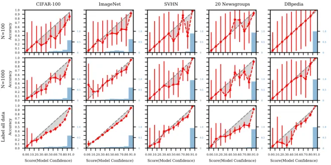
Another example of where we can apply Bayesian assessment is in assessing reliability diagrams for classifiers, a widely used tool for visually diagnosing model calibration (DeGroot and Fienberg, 1983; Niculescu-Mizil and Caruana, 2005) (e.g., Figure 2). These diagrams plot the empirical sample accuracyA(x) =p(y= ˆy|x)as a function of the model’s confidences(x) =pM(y= ˆy|x). If the model is perfectly calibrated, thenA(x) =s(x)and the diagram should plot the identity function on the diagonal. Any deviation away from the diagonal reflects miscalibration of the model. For a particular values(x) =s∈[0,1]along the x-axis, the correspondingy value is defined asEx|s(x)=s[A(x)]. As we did in the previous section, we model the marginal accuracy within each bin as an unknown quantityθj=Ep(x,y|x∈Rj)[A(x)]. We use a Beta prior over eachθj ∈[0,1], then update this prior using a binomial likelihood over binary observationsy∈[0,1].

In Figure 2, the prior distribution of marginal accuracy within each bin is a Beta distribution with its mean on the diagonal and pseudocountα+β= 2. As the amount of data used increases, the credible intervals of the Bayesian reliability diagram (left column) get narrower, the posterior density of ECE (right column) converges to ground truth, and the uncertainty about ECE decreases. When the number of samples is small, with the same set of randomly selected samples 100 samples (row 1), the Bayesian estimation of ECE puts non-negative probability mass on ground truth marginal ECE, where “ground truth" refers to the marginal ECE computed with all labeled assessment data, while the frequentist method significantly overestimates ECE without any notion of uncertainty.

(8)

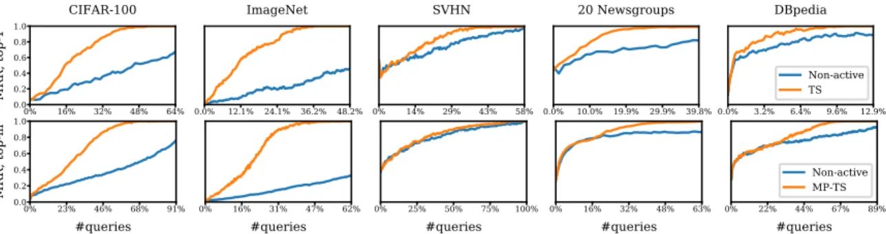
0.0% 7.5% 15.0% 22.5% 30.0% 0.0 0.2 0.4 0.6 0.8 1.0 MRR, top-1 CIFAR-100 0.0% 5.2% 10.4% 15.6% 20.8% ImageNet 0.0% 10.2% 20.4% 30.5% 40.7% SVHN 0.0% 4.0% 8.0% 11.9% 15.9% 20 Newsgroups 0.0% 1.6% 3.3% 4.9% 6.6% DBpedia TS Non-active 0% 15% 31% 46% 62% #queries 0.0 0.2 0.4 0.6 0.8 1.0 MRR, top-m 0.0% 7.4% 14.8% 22.2% 29.6%

#queries 0% 24%#queries47% 71% 95% 0.0% 9.0% 17.9% 26.9% 35.8%#queries 0% 14%#queries28% 41% 55%

MP-TS Non-active

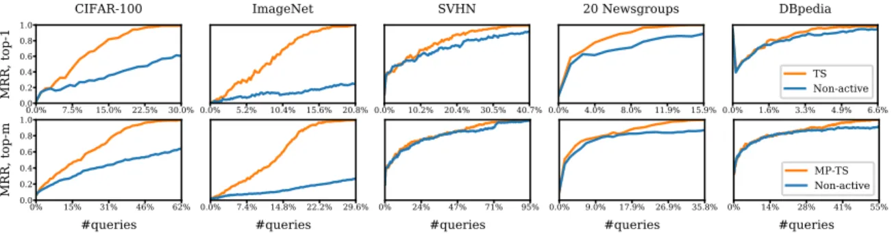
Figure 4: Mean reciprocal rank (MRR) of themlowest accuracy predicted classes, comparing active learning (with Thompson sampling (TS)) with no active learning, across five datasets. In

the top row m= 1, and in the bottom row m= 10for CIFAR-100 and ImageNet, and

m= 3for the other datasets.

0.0% 3.6% 7.2% 10.8% 14.4% #queries 0.0 0.2 0.4 0.6 0.8 1.0 MRR, top-1 ImageNet 0% 17% 35% 52% 69% #queries SVHN TS (informative) TS (uninformative)

Figure 5: Comparison of the effect of informative (green) and uninformative (orange) priors on identifying the least accurate predicted class on ImageNet and SVHN.

In Figure 3 we show the percentage error obtained for Bayesian mean posterior estimates (MPE) and frequentist estimates of marginal ECE as a function of the number of labeled data points (“queries") across five datasets. The percentage is computed relative to the ground truth marginal ECE=ECE∗. The MPE is computed with Monte Carlo samples from the posterior distribution (an example of histograms of such samples are shown in Figure 2). At each step, with we randomly draw and labelN queries from the pool of unlabeled data, and compute both a Bayesian and frequentist estimate of marginal calibration error with these labeled data. We run the simulation 100 times, and report the average ECEN over theN samples. Figure 2 plots(ECEN−ECE∗)/ECE∗ as a percentage. The Bayesian method consistently has lower ECE estimation error, especially when the number of queries is small.

4. Active Bayesian Assessment

The results in the previous section illustrate how the Bayesian approach can be useful in obtaining assessments with uncertainty quantification, e.g., for practical deployment situations where labeled data is likely to be sparse, in contrast to typical results in the literature which assume the availability of large test datasets for assessing performance metrics. In this section we illustrate how we can further improve performance by extending our Bayesian framework toactive assessment, allowing for model assessment to be performed by actively selecting examplesxfor labeling in a data-efficient manner. This scenario is particularly relevant to problems where we have a potentially large pool of unlabeled examplesxavailable, and have limited resources for labeling (e.g., a human labeler). The question we address here is, if we can only selectN classes from a larger pool of unlabeled examples, which examples should we select. We illustrate below how active data selection can be performed to

(9)

0 10 20 30 40 50 60 70 80 90 100 True label Human 0 10 20 30 40 50 60 70 80 90100 Predicted label 0 10 20 30 40 50 60 70 80 90 100 True label Superclass (a) 0.0 0.2 0.4 0.6 0.8 1.0 MRR, top-1 Human 0% 25% 50% 75% 100% #queries 0.0 0.2 0.4 0.6 0.8 1.0 MRR, top-1 Superclass Non-active TS (uninformative) TS (informative) (b) 0 10 20 30 40 50 60 70 80 90 True label Uninformative prior

N = 10 N = 1000 All labeled data

0 10 20 30 40 50 60 70 80 90 Predicted label 0 10 20 30 40 50 60 70 80 90 True label Informative prior 0 10 20 30 40 50 60 70 80 90

Predicted label 0 10 20 30 40 50 60 70 80 90100Predicted label (c)

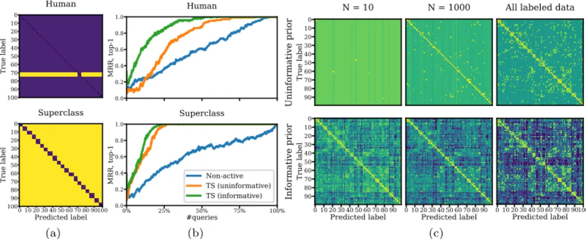
Figure 6: (a) Cost matrices used in our experiments. (top): misclassifying humans (the row in yellow) is 10x more costly than other mistakes. (bottom): confusing a class with another superclass (e.g., avehiclewith afish) is 10x more expensive than a mistake within the same superclass (e.g., confusingshark withtrout). (b) Success rates of active assessment using Thompson sampling (TS) (with both informative and uninformative priors) vs. non-active assessment for determining the predicted class with highest expected cost. Active learning with the informative prior detects the highest cost predicted class using far fewer queries than the other methods. (c) Comparison of the mean posterior estimates of the confusion probabilitiesθ (in the superclass experiment) under informative and uninformative priors.

solve the problem of identifying extreme classes (e.g., classes that rank first or the last according to a given metric such accuracy, calibration error, or expected cost)

4.1 Best Arm Identification

Thompson Sampling The problem of identifying extreme classes can be formulated as a multi-armed bandit problem where the “arms” are predicted classesyˆ, and the “reward” signal is a function of the model’s predictionyˆand true labely (e.g., +1 every timey6= ˆy if the goal is to determine the least accurate predicted class). The popular Thompson sampling algorithm used to solve this class of problems (Thompson, 1933; Russo et al., 2018) readily lends itself to our Bayesian framework. The basic idea is, at each query, to sample from the posterior distribution of the evaluation metric, and select one data pointxto be labeled (from a pool of unlabeled examples) for the predicted class (or arm) with highest/lowest sampled value.

We also experimented with a modified version of Thompson sampling called top-two Thompson sampling (TTTS) which has theoretical advantages for identifying the best arm in a pure exploration mode (Russo, 2016). This algorithm adds a re-sampling process to encourage more exploration. At each step, the second-most optimal arm may be randomly selected in place of the most optimal arm. We found that for the problems and datasets we investigated in this paper that TS and TTTS gave very similar performance, so we for simplicity we just present results for TS in this paper. A formal description of these algorithms is provided in the supplemental material.

There are a variety of other active learning algorithms (such as epsilon-greedy and UCB methods) that could also be used for active assessment. We found Thompson sampling to be more reliable and consistent in terms of efficiency than these methods across all five datasets (results and sensitivity analysis for prior strength in the supplementary material). We focus on the Bayesian/TS approach in

(10)

our results below since our primary aim is to demonstrate the utility of active assessment compared to no active assessment.

4.2 Best-m Arms Identification

Another variant of an active Bayesian assessment framework is best-marms identification.1 _{This can} be motivated for example by task allocation, e.g., finding thempredicted classes that a model is least accurate on, so that whenever the model predicts one of these classes the prediction decision is handed instead to a more accurate predictor (e.g., a human). For example, suppose we have a dataset withK= 100equally-likely classes (e.g., CIFAR-100) and a budget where we can send 10% of our examples to a human to make predictions (and the other 90% are made by our black-box model). One way to address this is to find the set of 10 predicted classes that the model is least accurate for and use the human to make predictions whenyˆis in this set.

Identification of the best-marms can be formulated as a multiple-play multi-armed bandit (MAB) problem. Komiyama et al. (2015) proposed the multiple-play Thompson sampling (MP-TS) algorithm and proved that MP-TS has the optimal regret upper bound when the reward is binary. This algorithm differs from standard Thompson sampling in that, at each step, data points for the top-m

arms (according to a sample from the posterior) are labeled as opposed to just the top arm. A detailed algorithm description is provided in the supplemental material.

4.3 Active Bayesian Assessment of Accuracy

We apply the active Bayesian assessment framework to the problem of determining the predicted classes with the lowest classwise accuracies, using the beta-binomial model described in Section 3.1. Figure 4 compares our active Bayesian assessment method to a traditional non-active assessment method (i.e., evaluating on a test set of uniformly drawn data points). Each algorithm was run 100 different times on each of the datasets listed in Table 1. For evaluation, for each run, at each step, we identify the least accurate classes, according to the MPE of the posterior distribution for the Bayesian method and the frequency-based estimate for the non-active method.

The x-axis measures the number of queries made to the oracle. The y-axis measures the mean reciprocal rank (MRR) of the predicted top-mclasses:

M RR= 1 m m X i=1 1 ranki (5)

where ranki is the predicted rank of theith best class. Following standard practice, other classes in the best-mare ignored when computing rank so that M RR= 1if the predicted top-mclasses match ground truth.

Our results demonstrate that the active learning approach is much more effective at identifying the least accurate class or least accurate top-mclasses relative to working with a randomly sampled test set. For example, for CIFAR-100 and ImageNet, in all of the trials, the correct class is identified after querying 30% and 20% of the pool of unlabeled data respectively. In contrast, the non-active strategy only gets MRR around 0.5 and 0.2 on these two datasets with the same amount of labeled data. In general, active assessment appears to achieve the largest gains in efficiency on datasets where the number of classes is large (e.g., CIFAR-100 and ImageNet).

Figure 4 shows the results when the prior distribution of accuracy is uninformative. However, since a model’s confidence reflects a model’s self-assessment of accuracy, we could also use an informative prior by placing a prior distribution for accuracy that is centered around the model’s confidence per class. Figure 5 shows the results for two data sets comparing active assessment for an informative prior (green) and an uninformative prior (orange). We set the uninformative prior for classwise

1. This is typically referred to as best-karms identification in the literature. We use the symbolmto avoid overloading

(11)

accuracy to be Beta(1,1)for each predicted class, the informative prior to be Beta(2sk,2(1−sk)), where sk is the average model confidence (score) of all data points (which we can obtain using unlabeled data) for the predicted class k. The results in Figure 5 illustrate that the informative prior can be helpful when the prior captures the relative ordering of classwise accuracy well (e.g., ImageNet), but less helpful when the difference in classwise accuracy across classes is small and the classwise ordering reflected in the “self-assessment prior" is more likely to be in error (e.g., SVHN; classwise accuracies provided in the supplementary material).

4.4 Active Bayesian Assessment of Confusion Matrices and Misclassification Costs

Accuracy assessment can be viewed as implicitly assigning a binary cost to model mistakes, i.e. a cost of 1 to incorrect predictions and a cost of 0 to correct predictions. In this sense, identifying the predicted class with lowest accuracy is equivalent to identifying the class with greatest expected cost. However, in real world applications, costs of different types of mistakes can vary drastically. For example, in autonomous driving applications, misclassifying a pedestrian as a crosswalk can have much more severe consequences than other misclassifications.

To deal with such situations, we extend our approach to incorporate an arbitrary cost matrix

C = [cjk], where cjk is the cost of predicting class yˆ = k for a data point whose true class is

y = j. Conditioned on a predicted class yˆ, the true class label y has a categorical distribution

θjk=p(y=j|yˆ=k). We will refer toθjk as confusion probabilities since they resemble the elements

of a confusion matrix. Theclasswise expected costfor predicted classkis given by:

CRk =Ep(x,y|x∈Rk)[cjk1(y=j)] = K

X

j=1

cjkθjk. (6)

Similar to how we use a beta-binomial distribution to model accuracy, we can model these confusion probabilities using a Dirichlet-multinomial distribution: θ·k ∼ Dirichlet(α·k). The same active querying approach described in the previous section can then be used to identify the class with the highest classwise expected cost (e.g.,k?_{= arg max}

kCRk).

For prior distributions we evaluate two options. The first is an uninformative prior with αjk=

α,∀j, k. The second is an informative prior based on the model’s own prediction scores, αjk ∝

Σx∈RkpM(y=j|x). This informative prior is likely to be more useful for problems such as CIFAR-100

where the number of confusion probabilities to estimate is large and observations are relatively sparse. We experiment with two different cost matrices on the CIFAR-100 dataset: (i) the cost of misclassifying a person (e.g., predictingfish when the true class is awoman,girl,boy, etc.) is more expensive than other mistakes, (ii) the cost of confusing a class with another superclass (e.g., a vehicle with afish) is more expensive than the cost of mistaking labels within the same superclass (e.g., confusingshark withtrout). We visualize these cost matrices in Figure 6(a). In Figure 6(b), we compare the performance of active and non-active assessment at identifying the class with highest cost, averaged over 100 trials. We set the pseudocount of both priors to be 1, and the cost of expensive mistakes to be 10x the cost of other mistakes. For both of the cost matrices we find that the active approach is more effective than the non-active approach, and that the informative prior is more effective than the uninformative prior. Even though the model is not well-calibrated (e.g., see Figures 1 and 2) there is nonetheless valuable information about confusion probabilities available from the model’s estimates of class-conditional probabilities.

To illustrate how the informative prior helps deal with sparsity, we plot samples from the posterior ofθwhen the number of queries is 10, 1000, 10000 in Figure 6(c). For the uninformative prior (top panel), even when all of the available data is used, there is still considerable uncertainty about the magnitude of the off-diagonal confusion probabilities. However, this is not the case for the informative prior (bottom panel) since the prior for the confusion probabilities more closely resembles the true confusion matrix.

(12)

0% 16% 32% 48% 64% 0.0 0.2 0.4 0.6 0.8 1.0 MRR, top-1 CIFAR-100 0.0% 12.1% 24.1% 36.2% 48.2% ImageNet 0% 14% 29% 43% 58% SVHN 0.0% 10.0% 19.9% 29.9% 39.8% 20 Newsgroups 0.0% 3.2% 6.4% 9.6% 12.9% DBpedia Non-active TS 0% 23% 46% 68% 91% #queries 0.0 0.2 0.4 0.6 0.8 1.0 MRR, top-m 0% 16% 31% 47% 62%

#queries 0% 25%#queries50% 75% 100% 0% 16%#queries32% 48% 63% 0% 22%#queries44% 67% 89%

Non-active MP-TS

Figure 7: Mean reciprocal rank (MRR) of themhighest ECE predicted classes, comparing active learning (with Thompson sampling (TS)) with no active learning, across five datasets. In

the top row m= 1, and in the bottom row m= 10for CIFAR-100 and ImageNet, and

m= 3for the other datasets.

Lastly, we investigate sensitivity of varying the relative cost of mistakes. We consistently observe that active assessment with an informative prior performs best, followed by active assessment with an uninformative prior and finally random sampling. Results are provided in the supplemental material.

4.5 Active Bayesian Assessment of Calibration

To identify classes for which the model is least calibrated (i.e., has lowest classwise ECE), we use the Bayesian model we proposed in Section 3 to actively assess classwise ECE of a model across different predicted classes. In Figure 7 we plot the average mean reciprocal rank (MRR) from 100 independent runs. As with classwise accuracy, active assessment can identify the correct top-mpredicted classes much more efficiently than the non-active approach, as a function of the number of label queries. The improvement in efficiency is particularly significant when the classwise calibration performance has large variance across the classes, e.g., CIFAR-100, ImageNet and 20 Newsgroups (additional details in the supplemental material).

5. Related Work

Prior work on using Bayesian ideas in the context of classifier assessment has tended to focus on very specific types assessment. Goutte and Gaussier (2005) propose a framework for Bayesian estimation of precision, recall, and F-score in an information retrieval context, and Johnson et al. (2019) use Bayesian mixture models to provide posterior distributions of diagnostic metrics (such as true positive rates) for medical tests. Benavoli et al. (2017) develop a general Bayesian framework for comparing multiple classifiers as an alternative to more traditional null hypothesis significance testing. We contribute to this body of work in two significant ways. Firstly, we expand the set of Bayesian diagnostics to a broader range of metrics, such as classwise accuracy and calibration metrics such as ECE and reliability diagrams. In addition, we develop approaches for the previously unstudied task ofactive assessment that are more label-efficient (and cost-effective) than traditional approaches which use fixed-size test sets or uniform sampling.

Other work has proposed frequentist methods for uncertainty quantification in an assessment context, e.g., resampling approaches such as the bootstrap for generating confidence intervals on calibration performance (Bröcker and Smith, 2007; Vaicenavicius et al., 2019). Our focus in this work is not to supplant these existing techniques, but instead to supplement them by providing an approach that includes the ability to incorporate of prior knowledge, and which readily lends itself to be used for active assessment.

(13)

While there is a large literature on active learning and multi-armed bandits (e.g., Settles (2012); Russo et al. (2018)), our paper is the first that applies these ideas to classifier assessment. In particular, our work builds on multi-armed bandit (MAB) inspired, pool-based active learning algorithms for data selection (Thompson, 1933; Russo, 2016; Komiyama et al., 2015). The techniques we use in this paper can in principle be replaced by any Bayesian active learning algorithms designed for MAB problems—determining the optimal active learning approach for model assessment is an interesting avenue for future research.

6. Conclusions

In this paper we described a Bayesian framework for assessing performance metrics of black-box classifiers, developing inference procedures for classwise accuracy, expected cost, and calibration metrics such as ECE. In addition, we proposed a new framework calledactive assessmentfor label-efficient assessment of classifier performance, and demonstrated its performance across five well-known datasets for identification of extreme classes such as the least accurate, least calibrated, or highest cost.

There are a number of interesting and useful directions for future work, such as Bayesian estimation of continuous functions related to accuracy and calibration (rather than over regions). The framework can also be extended to assess a particular model operating in multiple environments using a Bayesian hierarchical approach, or to comparatively assess multiple models operating in the same environment. A related direction is to consider environments where humans are in the loop where, given a constraint on the number of problems that can be allocated to humans, the goal is to identify for which types of prediction problems human accuracy will most likely exceed model accuracy.

(14)

Appendix A: Classwise ECE and Accuracy are Negatively Correlated

Figure 8 shows scatter plots of classwise accuracy and ECE assessed with our proposed Bayesian method for five datasets used in the paper. The assessment shows that model accuracy and calibration vary substantially across classes. For CIFAR-100, ImageNet and 20 Newsgroups, the variance of classwise accuracy and ECE among all predicted class is considerably greater than the variance of two other datasets. Figure 8 also illustrates that there is significant negative correlation between classwise accuracy and ECE across all 5 datasets, i.e. classes with low classwise accuracy also tend to be less calibrated. 0.50 0.75 1.00 Accuracy 0.1 0.2 0.3 ECE CIFAR-100 0.5 1.0 Accuracy 0.0 0.2 ImageNet 0.96 0.98 Accuracy 0.01 0.02 SVHN 0.6 0.8 1.0 Accuracy 0.0 0.1 0.2 ECE 20 Newsgroups 0.98 1.00 Accuracy 0.000 0.005 0.010 0.015 DBpedia

Figure 8: Scatter plots of classwise accuracy and ECE for 5 datasets. Each marker represents posterior means and 95% credible intervals of posterior accuracy and ECE for each predicted class. Markers in red and blue represent the top-m least and most accurate predicted classes, markers in gray represent the other classes, with m= 10for CIFAR-100 and ImageNet, andm= 3for the other datasets.

(15)

Appendix B: Bayesian Reliability Diagrams

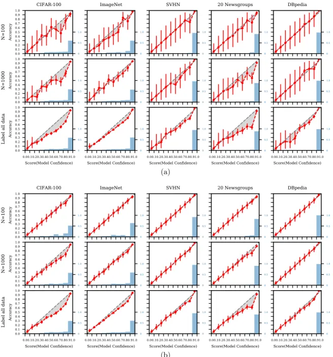
Figure 9 shows Bayesian reliability diagrams for five datasets, based on different amounts of labeled data. We used a Beta prior for each bin with αj =j/10 andβj = 1−j/10, j = 1, . . . ,10, i.e., a weak prior with pseudocountαj+βj= 1centered on the diagonal. Rows 1 and 2 display reliability diagrams estimated usingN = 100andN = 1000randomly selected examples (respectively). Row 3 displays diagrams estimated using the full set of available labeled examples for each dataset (e.g., the sizecolumn in Table 1).

With the full set of examples (row 3), the posterior means and the posterior 95% credible intervals are generally below the diagonal, i.e., we can infer with high confidence that the models are miscalibrated (and overconfident, to varying degrees) across all five datasets. For some bins where the scores are less than 0.5, the credible intervals are wide due to little data, and there is not enough information to determine with high confidence if the corresponding models are calibrated or not in these regions. With N = 100examples (row 1), the posterior uncertainty captured by the 95% credible intervals indicates that there is not yet enough information to determine whether the models are miscalibrated given onlyN = 100labeled examples. With N= 1000 examples (row 2) there is enough information to reliably infer that the CIFAR-100 model is overconfident in all bins for scores above 0.3. For the remaining datasets the credible intervals are generally wide enough to encompass 0.5 for most bins, meaning that we do not have enough data to make reliable inferences about calibration, i.e., the possibility that the models are well-calibrated cannot be ruled out without acquiring more data.

0.0 0.1 0.2 0.3 0.4 0.5 0.6 0.7 0.8 0.9 1.0 Accuracy N=100

CIFAR-100 ImageNet SVHN 20 Newsgroups DBpedia

0.0 0.1 0.2 0.3 0.4 0.5 0.6 0.7 0.8 0.9 1.0 Accuracy N=1000 0.00.10.20.30.40.50.60.70.80.91.0 Score(Model Confidence) 0.0 0.1 0.2 0.3 0.4 0.5 0.6 0.7 0.8 0.9 1.0 Accuracy

Label all data

0.00.10.20.30.40.50.60.70.80.91.0

Score(Model Confidence) 0.00.10.20.30.40.50.60.70.80.91.0Score(Model Confidence) 0.00.10.20.30.40.50.60.70.80.91.0Score(Model Confidence) 0.00.10.20.30.40.50.60.70.80.91.0Score(Model Confidence)

0 0.5 1.0 0 0.5 1.0 0 0.5 1.0 0 0.5 1.0 0 0.5 1.0 0 0.5 1.0 0 0.5 1.0 0 0.5 1.0 0 0.5 1.0 0 0.5 1.0 0 0.5 1.0 0 0.5 1.0 0 0.5 1.0 0 0.5 1.0 0 0.5 1.0

Figure 9: Bayesian reliability diagrams for five datasets (columns) estimated using varying amounts of test data (rows). The red circles plot the posterior mean for θj under our Bayesian model. Red bars display 95% credible intervals. Shaded gray areas indicate the estimated magnitudes of the calibration errors, relative to the Bayesian estimates. The blue histogram shows the distribution of the scores forN randomly drawn samples.

(16)

Appendix C: Inferring Statistics of Interest via Monte Carlo Sampling

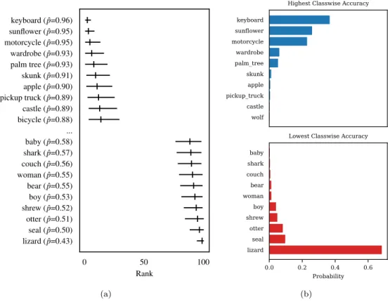
An additional benefit of the Bayesian framework is that we can draw samples from the posterior to infer other statistics of interest. Here we illustrate this method with two examples.

Bayesian Ranking via Monte Carlo Sampling We can infer the Bayesian ranking of classes in terms of classwise accuracy or expected calibration error(ECE), by drawing samples from the posterior distributions. For instance, we can estimate the ranking of classwise accuracy of a model for CIFAR-100, by sampling Aˆk’s (from their respective posterior Beta densities) for each of the classes and then compute the rank of each class with the sampled accuracy. We run this experiment 10,000 times and then for each class we can empirically estimate the distribution of its ranking. The MPE and 95% credible interval of ranking per predicted class for top 10 and bottom 10 are provided in Figure 10a for CIFAR-100.

0 50 100 Rank lizard ( ˆp=0.43) seal ( ˆp=0.50) otter ( ˆp=0.51) shrew ( ˆp=0.52) boy ( ˆp=0.53) bear ( ˆp=0.55) woman ( ˆp=0.55) couch ( ˆp=0.56) shark ( ˆp=0.57) baby ( ˆp=0.58) ... bicycle ( ˆp=0.88) castle ( ˆp=0.89) pickup truck ( ˆp=0.89) apple ( ˆp=0.90) skunk ( ˆp=0.91) palm tree ( ˆp=0.93) wardrobe ( ˆp=0.93) motorcycle ( ˆp=0.95) sunflower ( ˆp=0.95) keyboard ( ˆp=0.96) (a) keyboard sunflower motorcycle wardrobe palm_tree skunk apple pickup_truck castle wolf

Highest Classwise Accuracy

0.0 0.2 0.4 0.6 Probability lizard seal otter shrewboy woman bear couch sharkbaby

Lowest Classwise Accuracy

(b)

Figure 10: (a) MCMC-based ranking of accuracy across predicted classes for CIFAR-100 (where 1 corresponds to the class with the highest accuracy. (b) Posterior probabilities of the most and least accurate predictions on CIFAR-100. The class with the highest classwise accuracy is somewhat uncertain, while the class with the lowest classwise accuracy is very likelylizard.

Posterior probabilities of the most and least accurate predictions We can estimate the probability that a particular class such aslizard is the least accurate predicted class of CIFAR-100 by samplingAˆk∗’s (from their respective posterior Beta densities) for each of the classes and then measuring whetherAˆlizard is the minimum of the sampled values. Running this experiment 10,000 times and then averaging the results, we determine that there is a 68% chance that lizard is the least

(17)

accurate class predicted by ResNet-110 on CIFAR-100. The posterior probabilities for other classes are provided in Figure 10b, along with results for estimating which class has the highest classwise accuracy.

Appendix D: Different Multi-Armed Bandit Algorithms

Below we provide brief descriptions and pseudocode for the different variants of multi-armed bandit algorithm for the best arm or top-m arms identification we investigated in this paper, including Thompson Sampling(TS), Top-Two Thompson Sampling(TTTS), and multiple-play Thompson sampling(MP-TS)(Thompson, 1933; Russo, 2016; Komiyama et al., 2015).

Best Arm Identification Thompson sampling(TS) is a widely used method for online learning of multi-armed problems. The algorithm samples actions according to the posterior probability that they are optimal. Top-two Thompson sampling(TTTS)is a modified version of TS that is tailored for best-arm identification, and has some theoretical advantages. This algorithm adds a re-sampling process to encourage more exploration. Algorithm 1 and 2 describe the sampling process for identifying the most accurate predicted class with TS and TTTS.Kis the number of classes and Beta(α, β)is the prior distribution ofAk.

Top-m Arms Identification Multiple-play Thompson sampling(MP-TS)is an extension of TS to the multiple-play multi-armed bandit problem and it has a theoretical optimal regret guarantee with binary rewards. Algorithm 3 is the sampling process to identify the top-m arms with MP-TS, where

mis the number of best arms to identify.

Algorithm 1Thompson Sampling (TS) Strategy

Input: prior hyperparametersα,β

initializenk,0=nk,1= 0fork= 1toK repeat fork= 1to Kdo ˆ Ak ∼Beta(α+nk,0, β+nk,1) end for k∗= arg minkAˆ1:K

select data point(x,yˆ=k∗), query oracle for true label y

if y=k∗then

nk∗_,₀←n_k∗_,₀+ 1

else

nk∗_,₁←n_k∗_,₁+ 1

end if

(18)

Algorithm 2Top Two Thompson Sampling (TTTS) Strategy

initializenk,0=nk,1= 0fork= 1toK repeat fork= 1to Kdo ˆ Ak ∼Beta(α+nk,0, β+nk,1) end for

I= arg minkAˆ1:K,B∼Bernoulli(β)

if B= 1then k∗=I else repeat fork= 1to Kdo ˆ Ak∼Beta(α+nk,0, β+nk,1) end for J = arg minkAˆ1:K untilJ 6=I k∗=J end if

select data point(x,yˆ=k∗), query oracle for true label y

if y=k∗then

nk∗_,₀←n_k∗_,₀+ 1

else

nk∗_,₁←n_k∗_,₁+ 1

end if

untilall data labeled

Algorithm 3Multiple-play Thompson sampling (MP-TS) Strategy

initializenk,0=nk,1= 0fork= 1toK repeat fork= 1to Kdo ˆ Ak ∼Beta(α+nk,0, β+nk,1) end for

I∗=top-m arms ranked byAˆk.

fork∗ ∈I∗do

select data point(x,yˆ=k∗_{), query oracle for true label} _y

if y=k∗ _then nk∗_,₀←n_k∗_,₀+ 1 else nk∗_,₁←n_k∗_,₁+ 1 end if end for

(19)

Appendix E: Derivation of Classwise Expected Cost

Suppose we are given a modelM producing probability estimatespM(y|x), and cost-matrixC={cjk} where cjk is the cost of predicting classyˆ=kfor a data point whose true class isy=j. Conditioned on a predicted classyˆ, the true class label yhas a categorical distributionp(y=j|yˆ=k) =θjk. The classwise expected cost for predicted classkis given by,

(20)

Appendix F: Sensitivity Analysis for Hyperparameters

In Figure 11, we show Bayesian reliability diagrams for five datasets as the strength of the prior increases from 10 to 100. As the strength of the prior increases, it takes more labeled data to overcome the prior belief that the model is calibrated. In Figure 12, we show MRR of themlowest accurate predicted classes as the strength of the prior increases from 2 to 10 to 100. And in Figure 13, we show MRR of them least calibrated predicted classes as the strength of the prior increase from 2 to 5 and 10. From these plots, the proposed approach appears to be relatively robust to the prior strength.

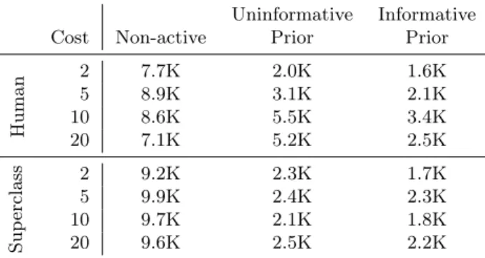
We also investigate the sensitivity of varying the relative cost of mistakes. Results are provided in Table 2. We consistently observe that active assessment with an informative prior performs the best, followed by active assessment with an uninformative prior and finally random sampling.

Uninformative Informative Cost Non-active Prior Prior

Human 2 7.7K 2.0K 1.6K 5 8.9K 3.1K 2.1K 10 8.6K 5.5K 3.4K 20 7.1K 5.2K 2.5K Sup erclass 2 9.2K 2.3K 1.7K 5 9.9K 2.4K 2.3K 10 9.7K 2.1K 1.8K 20 9.6K 2.5K 2.2K

Table 2: Number of queries required by different methods to achieve a 0.95 mean reciprocal rank(MRR) identifying the class with highest classwise expected cost. A pseudocount of 1 is used in the priors for Bayesian models.

(21)

0.0 0.1 0.2 0.3 0.4 0.5 0.6 0.7 0.8 0.9 1.0 Accuracy N=100

Label all data

0.00.10.20.30.40.50.60.70.80.91.0

0 0.5 1.0 0 0.5 1.0 0 0.5 1.0 0 0.5 1.0 0 0.5 1.0 0 0.5 1.0 0 0.5 1.0 0 0.5 1.0 0 0.5 1.0 0 0.5 1.0 0 0.5 1.0 0 0.5 1.0 0 0.5 1.0 0 0.5 1.0 0 0.5 1.0 (a) 0.0 0.1 0.2 0.3 0.4 0.5 0.6 0.7 0.8 0.9 1.0 Accuracy N=100

Label all data

0.00.10.20.30.40.50.60.70.80.91.0

0 0.5 1.0 0 0.5 1.0 0 0.5 1.0 0 0.5 1.0 0 0.5 1.0 0 0.5 1.0 0 0.5 1.0 0 0.5 1.0 0 0.5 1.0 0 0.5 1.0 0 0.5 1.0 0 0.5 1.0 0 0.5 1.0 0 0.5 1.0 0 0.5 1.0 (b)

Figure 11: Bayesian reliability diagrams for five datasets (columns) estimated using varying amounts of test data (rows) with prior strength (αj+βj for each bin) set to be (a) 10 and (b) 100 respectively. The red circles plot the posterior mean for θj under our Bayesian approach. Red bars display 95% credible intervals. Shaded gray areas indicate the estimated magnitudes of the calibration errors, relative to the Bayesian estimates. The blue histogram shows the distribution of the scores forN randomly drawn samples.

(22)

0.0% 7.5% 15.0% 22.5% 30.0% 0.0 0.2 0.4 0.6 0.8 1.0 MRR, top-1 CIFAR-100 0.0% 5.2% 10.4% 15.6% 20.8% ImageNet 0.0% 10.2% 20.4% 30.5% 40.7% SVHN 0.0% 4.0% 8.0% 11.9% 15.9% 20 Newsgroups 0.0% 1.6% 3.3% 4.9% 6.6% DBpedia TS Non-active 0% 15% 31% 46% 62% #queries 0.0 0.2 0.4 0.6 0.8 1.0 MRR, top-m 0.0% 7.4% 14.8% 22.2% 29.6%

MP-TS Non-active (a) 0.0% 7.7% 15.5% 23.2% 31.0% 0.0 0.2 0.4 0.6 0.8 1.0 MRR, top-1 CIFAR-100 0.0% 6.0% 12.0% 18.0% 24.0% ImageNet 0.0% 9.3% 18.6% 27.9% 37.3% SVHN 0.0% 4.0% 8.0% 11.9% 15.9% 20 Newsgroups 0.0% 1.6% 3.3% 4.9% 6.6% DBpedia TS Non-active 0% 16% 31% 47% 63% #queries 0.0 0.2 0.4 0.6 0.8 1.0 MRR, top-m 0% 25% 50% 75% 100%

MP-TS Non-active (b) 0.0% 9.2% 18.5% 27.7% 37.0% 0.0 0.2 0.4 0.6 0.8 1.0 MRR, top-1 CIFAR-100 0.0% 7.0% 14.0% 21.0% 28.0% ImageNet 0% 14% 28% 42% 56% SVHN 0.0% 6.3% 12.6% 18.9% 25.2% 20 Newsgroups 0.0% 3.5% 7.0% 10.5% 14.0% DBpedia TS Non-active 0% 19% 37% 56% 75% #queries 0.0 0.2 0.4 0.6 0.8 1.0 MRR, top-m 0% 25% 50% 75% 100%

MP-TS Non-active

(c)

Figure 12: Mean reciprocal rank (MRR) of themclasses with the estimated lowest classwise accuracy as the strength of the prior varies from (a) 2 to (b) 10 and (c) 100, comparing active learning (with Thompson sampling (TS)) with no active learning, across five datasets. For each of (a), (b) and (c), in the upper rowm= 1, and in the lower row m= 10for CIFAR-100 and ImageNet, andm= 3for the other datasets.

(23)

0% 16% 32% 48% 64% 0.0 0.2 0.4 0.6 0.8 1.0 MRR, top-1 CIFAR-100 0.0% 12.1% 24.1% 36.2% 48.2% ImageNet 0% 14% 29% 43% 58% SVHN 0.0% 10.0% 19.9% 29.9% 39.8% 20 Newsgroups 0.0% 3.2% 6.4% 9.6% 12.9% DBpedia Non-active TS 0% 23% 46% 68% 91% #queries 0.0 0.2 0.4 0.6 0.8 1.0 MRR, top-m 0% 16% 31% 47% 62%

Non-active MP-TS (a) 0% 18% 36% 53% 71% 0.0 0.2 0.4 0.6 0.8 1.0 MRR, top-1 CIFAR-100 0% 18% 37% 55% 74% ImageNet 0% 15% 31% 46% 62% SVHN 0.0% 10.3% 20.7% 31.0% 41.3% 20 Newsgroups 0.0% 3.5% 7.0% 10.5% 14.0% DBpedia Non-active TS 0% 24% 47% 71% 94% #queries 0.0 0.2 0.4 0.6 0.8 1.0 MRR, top-m 0% 20% 41% 61% 81%

Non-active MP-TS (b) 0% 21% 42% 62% 83% 0.0 0.2 0.4 0.6 0.8 1.0 MRR, top-1 CIFAR-100 0% 23% 47% 70% 94% ImageNet 0% 17% 34% 51% 68% SVHN 0.0% 11.4% 22.9% 34.3% 45.7% 20 Newsgroups 0.0% 4.8% 9.5% 14.3% 19.0% DBpedia Non-active TS 0% 25% 50% 75% 100% #queries 0.0 0.2 0.4 0.6 0.8 1.0 MRR, top-m 0% 25% 49% 74% 98%

Non-active MP-TS

(c)

Figure 13: Mean reciprocal rank (MRR) of themclasses with the estimated highest classwise ECE as the strength of the prior varies from (a) 2 to (b) 5 and (c) 10, comparing active learning (with Thompson sampling (TS)) with no active learning, across five datasets. For each of (a), (b) and (c), in the upper rowm= 1, and in the lower rowm= 10for CIFAR-100

(24)

References

Alessio Benavoli, Giorgio Corani, Janez Demšar, and Marco Zaffalon. Time for a change: a tutorial for comparing multiple classifiers through Bayesian analysis. The Journal of Machine Learning Research, 18(1):2653–2688, 2017.

Jochen Bröcker and Leonard A Smith. Increasing the reliability of reliability diagrams. Weather and Forecasting, 22(3):651–661, 2007.

Morris H DeGroot and Stephen E Fienberg. The comparison and evaluation of forecasters. Journal of the Royal Statistical Society: Series D (The Statistician), 32(1-2):12–22, 1983.

Jacob Devlin, Ming-Wei Chang, Kenton Lee, and Kristina Toutanova. BERT: Pre-training of deep bidirectional transformers for language understanding. InNAACL-HLT 2019, volume 1, pages 4171–4186, 2019.

Xianzhi Du, Mostafa El-Khamy, Jungwon Lee, and Larry Davis. Fused DNN: A deep neural network fusion approach to fast and robust pedestrian detection. InWinter Conference on Applications of Computer Vision, pages 953–961, 2017.

Yarin Gal and Zoubin Ghahramani. Dropout as a Bayesian approximation: Representing model uncertainty in deep learning. InInternational Conference on Machine Learning, pages 1050–1059, 2016.

Cyril Goutte and Eric Gaussier. A probabilistic interpretation of precision, recall and F-score, with implication for evaluation. InEuropean Conference on Information Retrieval, pages 345–359, 2005. Chuan Guo, Geoff Pleiss, Yu Sun, and Kilian Q Weinberger. On calibration of modern neural

networks. InInternational Conference on Machine Learning, pages 1321–1330, 2017.

Kaiming He, Xiangyu Zhang, Shaoqing Ren, and Jian Sun. Deep residual learning for image recognition. InComputer Vision and Pattern Recognition, pages 770–778, 2016.

Dan Hendrycks and Kevin Gimpel. A baseline for detecting misclassified and out-of-distribution examples in neural networks. InInternational Conference on Learning Representations, 2017. Wesley O Johnson, Geoff Jones, and Ian A Gardner. Gold standards are out and Bayes is in:

Implementing the cure for imperfect reference tests in diagnostic accuracy studies. Preventive Veterinary Medicine, 167:113–127, 2019.

Daniel S Kermany, Michael Goldbaum, Wenjia Cai, Carolina CS Valentim, Huiying Liang, Sally L Baxter, Alex McKeown, Ge Yang, Xiaokang Wu, Fangbing Yan, et al. Identifying medical diagnoses and treatable diseases by image-based deep learning. Cell, 172(5):1122–1131, 2018.

Junpei Komiyama, Junya Honda, and Hiroshi Nakagawa. Optimal regret analysis of Thompson sampling in stochastic multi-armed bandit problem with multiple plays. InInternational Conference on Machine Learning, pages 1152–1161, 2015.

Alex Krizhevsky and Geoffrey Hinton. Learning multiple layers of features from tiny images. Technical report, Citeseer, 2009.

Meelis Kull, Telmo Silva Filho, and Peter Flach. Beta calibration: a well-founded and easily implemented improvement on logistic calibration for binary classifiers. InArtificial Intelligence and Statistics, pages 623–631, 2017.

Ananya Kumar, Percy S Liang, and Tengyu Ma. Verified uncertainty calibration. InAdvances in Neural Information Processing Systems, pages 3787–3798, 2019.

(25)

Balaji Lakshminarayanan, Alexander Pritzel, and Charles Blundell. Simple and scalable predictive uncertainty estimation using deep ensembles. In Advances in Neural Information Processing Systems, pages 6402–6413, 2017.

Ken Lang. Newsweeder: Learning to filter netnews. InMachine Learning Proceedings, pages 331–339. Elsevier, 1995.

Zachary C Lipton, Yu-Xiang Wang, and Alex Smola. Detecting and correcting for label shift with black box predictors. InInternational Conference on Machine Learning, pages 3128–3136, 2018. Yuval Netzer, Tao Wang, Adam Coates, Alessandro Bissacco, Bo Wu, and Andrew Y Ng. Reading

digits in natural images with unsupervised feature learning. NIPS Workshop on Deep Learning and Unsupervised Feature Learning, 2011.

Alexandru Niculescu-Mizil and Rich Caruana. Predicting good probabilities with supervised learning. InInternational Conference on Machine Learning, pages 625–632, 2005.

Jeremy Nixon, Michael W. Dusenberry, Linchuan Zhang, Ghassen Jerfel, and Dustin Tran. Measuring calibration in deep learning. InThe IEEE Conference on Computer Vision and Pattern Recognition Workshops, June 2019.

Yaniv Ovadia, Emily Fertig, Jie Ren, Zachary Nado, D Sculley, Sebastian Nowozin, Joshua V Dillon, Balaji Lakshminarayanan, and Jasper Snoek. Can you trust your model’s uncertainty? evaluating predictive uncertainty under dataset shift. InAdvances in Neural Information Processing Systems, pages 13969–13980, 2019.

Benjamin Recht, Rebecca Roelofs, Ludwig Schmidt, and Vaishaal Shankar. Do imagenet classifiers generalize to imagenet? InInternational Conference on Machine Learning, pages 5389–5400, 2019. Olga Russakovsky, Jia Deng, Hao Su, Jonathan Krause, Sanjeev Satheesh, Sean Ma, Zhiheng Huang, Andrej Karpathy, Aditya Khosla, Michael Bernstein, et al. Imagenet large scale visual recognition challenge. International Journal of Computer Vision, 115(3):211–252, 2015.

Daniel Russo. Simple Bayesian algorithms for best arm identification. InConference on Learning Theory, pages 1417–1418, 2016.

Daniel J Russo, Benjamin Van Roy, Abbas Kazerouni, Ian Osband, Zheng Wen, et al. A tutorial on thompson sampling. Foundations and Trends in Machine Learning, 11(1):1–96, 2018.

Burr Settles. Active Learning. Synthesis Lectures on AI and ML. Morgan Claypool, 2012.

William R Thompson. On the likelihood that one unknown probability exceeds another in view of the evidence of two samples. Biometrika, 25(3/4):285–294, 1933.

Juozas Vaicenavicius, David Widmann, Carl Andersson, Fredrik Lindsten, Jacob Roll, and Thomas Schön. Evaluating model calibration in classification. InInternational Conference on Artificial Intelligence and Statistics, pages 3459–3467, 2019.

Yuanshun Yao, Zhujun Xiao, Bolun Wang, Bimal Viswanath, Haitao Zheng, and Ben Y Zhao. Complexity vs. performance: empirical analysis of machine learning as a service. In Internet Measurement Conference, pages 384–397, 2017.

Bianca Zadrozny and Charles Elkan. Transforming classifier scores into accurate multiclass probability estimates. InInternational Conference on Knowledge Discovery and Data Mining, pages 694–699, 2002.

Xiang Zhang, Junbo Zhao, and Yann LeCun. Character-level convolutional networks for text classification. InAdvances in Neural Information Processing Systems, pages 649–657, 2015.