Computational methods for hidden Markov tree models
- An application to wavelet trees.
Jean-Baptiste Durand, Paulo Goncalv`
es, Yann Gu´
edon
To cite this version:
Jean-Baptiste Durand, Paulo Goncalv`es, Yann Gu´edon. Computational methods for hid-den Markov tree models - An application to wavelet trees.. IEEE Transactions on Sig-nal Processing, Institute of Electrical and Electronics Engineers, 2004, 52 (9), pp.2551-2560.
<10.1109/TSP.2004.832006>. <hal-00830078>
HAL Id: hal-00830078
https://hal.inria.fr/hal-00830078
Submitted on 4 Jun 2013
HAL is a multi-disciplinary open access archive for the deposit and dissemination of sci-entific research documents, whether they are pub-lished or not. The documents may come from teaching and research institutions in France or abroad, or from public or private research centers.
L’archive ouverte pluridisciplinaire HAL, est destin´ee au d´epˆot et `a la diffusion de documents scientifiques de niveau recherche, publi´es ou non, ´emanant des ´etablissements d’enseignement et de recherche fran¸cais ou ´etrangers, des laboratoires publics ou priv´es.
Computational Methods for Hidden Markov Tree Models –
An Application to Wavelet Trees
Jean-Baptiste Durand ∗ Paulo Gon¸calv`es † Yann Gu´edon ‡
August 26, 2004
Abstract: The hidden Markov tree models were introduced by Crouse, Nowak and Baraniuk in 1998 for modeling nonindependent, non-Gaussian wavelet transform coeffi-cients. In their article, they developed the equivalent of the forward-backward algorithm for hidden Markov tree models and termed it the “upward-downward algorithm”. This algorithm is subject to the same numerical limitations as the forward-backward algorithm for hidden Markov chains. In this paper, adapting the ideas of Devijver from 1985, we propose a new “upward-downward” algorithm, which is a true smoothing algorithm and is immune to numerical underflow. Furthermore, we propose a Viterbi-like algorithm for global restoration of the hidden state tree. The contribution of those algorithms as diag-nosis tools is illustrated through the modeling of statistical dependencies between wavelet coefficients with a special emphasis on local regularity changes.
Keywords: hidden Markov tree model, EM algorithm, hidden state tree restoration, upward-downward algorithm, wavelet decomposition, scaling laws, change detection
1
Introduction
The hidden Markov tree models (HMT) were introduced by Crouse, Nowak and Baraniuk (1998) [6]. The context of their work was the modeling of statistical dependencies between wavelet coefficients in signal processing, for which observations are organized in a tree structure. Applications of such models are: image segmentation, signal classification, denoising and image document categorization; see Choi and Baraniuk (1999) [4], and Diligenti, Frasconi and Gori (2001) [9]. Dasgputa et al. (2001) [7] used a mixture of
∗InriaRhˆone-Alpes, Montbonnot, France - email :[email protected] †InriaRhˆone-Alpes, Montbonnot, France - email :[email protected] ‡Cirad, Montpellier, France - email :[email protected]
hidden Markov trees with a Markovian regime for target classification using measured acoustic scattering data.
These models share similarities with hidden Markov chains (HMCs): both are models with hidden states, parameterized by a transition probability matrix and emission (or observation) distributions. Both models can be identified through the EM algorithm, involving two recursions acting in opposite directions. In both cases, these recursions involve probabilities that tend toward zero exponentially fast, causing underflow problems on computers.
The use of hidden Markov models (HMMs) relies on two main algorithms, namely, the smoothing algorithm and the global restoration algorithm. The former computes the probabilities of being in statej at nodeugiven all the observed data. These probabilities, as a function of the index parameteru, constitute a relevant diagnosis tool; see Churchill (1989) [5] in the context of DNA sequence analysis. The smoothing algorithm also enables an efficient implementation of the E step of the EM algorithm. In most applications, the knowledge of the hidden states provides an interpretation of the data, based on the model. This motivates the need for the latter algorithm. The aim of this paper is to provide a smoothing algorithm, which is immune to underflow, and a solution for the global hidden state tree restoration.
Thus, we derive a smoothing algorithm for the HMT model, adapted from the forward-backward algorithm of Devijver (1985) [8] for HMCs. This algorithm is based on a direct decomposition of the smoothed probabilities. However the adaptation to hidden Markov tree models is not straightforward and the resulting algorithm requires an additional re-cursion consisting in computing the hidden state marginal distributions. Then, we present the Viterbi algorithm for HMT models. We show that the well-known Viterbi algorithm for HMCs cannot be adaptated to the HMT model. Thus, we propose a Viterbi algorithm for HMCs based on a backward recursion, which appears as a building block of thehybrid restoration algorithm of Brushe et al. (1988) [3]. This the basis for our HMT Viterbi algorithm.
Thereafter, for illustrative purpose, we apply our proposed algorithms to a segmen-tation problem, a standard and yet difficult signal processing task. This canonical study echoes a host of real world situations (image processing, network traffic analysis,
biomedi-cal engineering,. . . ) where the classifying parameter is the lobiomedi-cal regularity of the measure. Wavelets have proved particularly efficient at estimating this parameter, and we show how our upward-downward algorithm circumvents the underflow problem that generally precludes classical approaches from applying to large data sets. In a second step, we elaborate on a specific use of the smoothing algorithm we propose, and principally, we motivate the usefulness of probabilistic maps when the local regularity is no longer a deterministic parameter, but the realization of a random variable with unknown density (e.g., multifractals).
This paper is organized as follows. The hidden Markov tree models are introduced in Section 2. The upward-downward algorithm of Crouse et al. (1998) [6] is summarized in Section 3. A parallel is drawn between theforward-backwardalgorithm for hidden Markov chains and their algorithm, which is shown to be subject to underflow. Then we give an
upward-downwardalgorithm using smoothed probabilities for hidden Markov tree models. A solution for the global restoration problem is proposed in Section 4. An application based on simulations is provided in Section 5. This illustrates the importance of the HMT model and that of our algorithms in signal processing. Section 6 consists of concluding remarks.
2
The Hidden Markov Tree model
We use the general notationP() to denote either a probability mass function or a probabil-ity densprobabil-ity function, the true nature ofP() being obvious from the context. This notation obviates any assumption on the discrete or continuous nature of the output process.
Let X¯1 = (X1, . . . , Xn) be the output process, which is assumed to be indexable as a tree rooted in X1. An hidden Markov tree model is composed of the observed random
tree (X1, . . . , Xn) and a hidden random tree (S1, . . . , Sn), which has the same indexing
structure as the observed tree. The variables Su are discrete with K states, denoted
{1, . . . , K}. These variables can be indexed as a tree rooted in S1. This model can be
considered to be an unobservable state process S¯1, called a Markov tree and is related to the “output” treeX¯1by a probabilistic mapping parameterized by observation or emission distributions.
foru6= 1. We also introduce the following notations.
• X¯u = x¯u is the observed subtree rooted at node u. Thus X¯1 = x¯1 is the entire observed tree;
• X¯c(u)=x¯c(u) denotes the collection of observed subtrees rooted at children of node
u (that is the subtree x¯u except its rootxu);
• if X¯u is a proper subtree of X¯v then X¯v\u =x¯v\u is the subtree rooted at node v except the subtree rooted at node u;
• X¯1\c(u) = x¯1\c(u) denotes the entire tree except the subtrees rooted at children of node u.
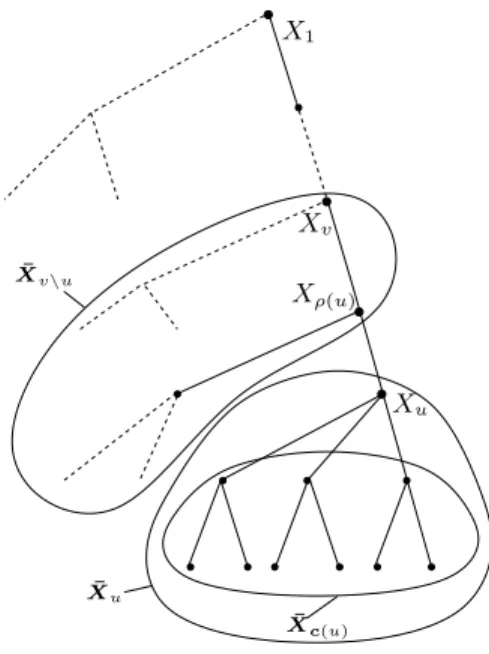
These notations, xhich are illustrated in Figure 1, transpose to the hidden state tree, with, for instance,S¯u =s¯u, the state subtree rooted at nodeu.
Xv X1 ¯ Xv\u Xu ¯ Xc(u) Xρ(u) ¯ Xu
Figure 1: Notations used for indexing trees.
A distribution P() is said to satisfy the hidden Markov tree property if and only if it fulfills the following two assumptions.
• ∀u∈ {1, . . . , n},Xu arise from a mixture of distributions with probability
P(Xu =x) = K
X
j=1
• factorization property: ∀(x¯1,s¯1), P(X¯1=x¯1,S¯1 =s¯1) =P(S1 =s1) Y u6=1 P(Su =su|Sρ(u)=sρ(u)) Y u P(Xu=xu|Su=su). (1)
The influence diagram is a graphical way for describing conditional independence re-lations between random variables; see Smyth, Heckerman and Jordan (1997) [21]. The influence diagram corresponding to HMT models is shown in Figure 2. The conditional independence properties of the HMT models can be deduced from the factorization prop-erty (1). S1 Xu Su X1 Sρ(u) Xρ(u)
Figure 2: Influence diagram for hidden Markov tree models.
An hidden Markov tree model (X¯1,S¯1) is defined by the following parameters:
• the initial distribution π = (πj)j = (P(S1 = j))j for the root node S1 and the
transition probabilities P = (pij)i,j defined bypij =P(Su =j|Sρ(u) =i);
• the parameters of the emission distributions (θ1, . . . , θK), such as
P(Xu=x|Su=j) =Pθj(x),
where Pθ belongs to a parametric distribution family. We call them the emission
parameters. For example,Pθcan be a Gaussian distribution. In this case,θ= (µ,Σ)
Crouseet al. (1998) [6] considered the possibility that transition probability matrices and emission parameters depend on nodeu. These models do not enable a reliable estimation using only one observed tree x¯1, as discussed by the authors. Thus, we directly consider homogeneous models(i.e. models having transition probabilities and emission parameters independent ofu), which is usual in the literature of hidden Markov models. Our results can be easily extended to non-homogeneous models, at the cost of tedious notation.
3
Upward-downward algorithm
Since the state tree S¯1 is not observable, the EM algorithm is a natural way to obtain maximum likelihood estimates of a HMT. The E step requires the computation of the con-ditional distributionsξu(j) =P(Su =j|X¯1 =x¯1) (smoothed probabilities) and P(Su =
j, Sρ(u) =i|X¯1 =x¯1). Crouse et al. (1998) [6] proposed the so-called upward-downward algorithm to calculate these quantities, which basically computes P(Su = j,X¯1 = x¯1)
for each node u and each state j. This is a direct transposition to the HMT context of the forward-backward algorithm for hidden Markov chains proposed by Baum et al.
(1970) [2]. Both the upward-downward and the forward-backward algorithms suffer from underflow problems; see Ephraim and Merhav (2002) [10] for the case of hidden Markov chains. This difficulty has been initially overcome by Levinson et al. (1983) [14], who proposed the use of scaling factors on rather heuristic grounds. On the basis of this work, Devijver (1985) [8] derived a true smoothing algorithm for hidden Markov chains, which can be interpreted in the setting of state space models. This motivates the need for a true smoothing algorithm for HMT models with the following properties:
• the smoothed probabilities P(Su = j|X¯1 = x¯1) are computed instead of P(Su =
j,X¯1 = x¯1). These quantities are also useful diagnosis tools for HMT models, as will be shown in the application (section 5);
• the probabilities P(Su = j, Sρ(u) =i|X¯1 =x¯1) can be directly extracted from this
smoothing algorithm. Consequently, it implements the E step of the EM algorithm for parameter estimation;
3.1 Upward-downward algorithm of Crouse, Nowak and Baraniuk (1998)
Its objective is to compute the probabilityP(Su=j,X¯1=x¯1) for each nodeu and each
statej. The authors define the following quantities: ˜ βu(j) = P(X¯u=x¯u|Su =j); ˜ βρ(u),u(j) = P(X¯u=x¯u|Sρ(u)=j); ˜ αu(j) = P(Su=j,X¯1\u =x¯1\u).
Their algorithm is based on the following decomposition of the joint probabilities:
P(Su=j,X¯1=x¯1) = P(X¯u =x¯u|Su=j)P(Su =j,X¯1\u =x¯1\u)
= β˜u(j)˜αu(j).
Theupward and downwardrecursions, based on the algorithm of Ronen et al. (1995) [20] for Markov trees with missing data, are defined as follows:
Upward recursion ˜ βu(j) =P(X¯u=x¯u|Su =j) = Y v∈c(u) P(X¯v =x¯v|Su=j) P(Xu=xu|Su=j) = Y v∈c(u) ˜ βu,v(j) Pθj(xu); (2) ˜ βρ(u),u(j) =P(X¯u =x¯u|Sρ(u)=j) = X k P(X¯u =x¯u|Su=k)P(Su =k|Sρ(u)=j) = X k ˜ βu(k)pjk. (3)
Since, from the equations above, the computation of ˜βu(j) requires the quantities ( ˜βv(k))k
for each child v of u, this procedure can be implemented by an upward inductive tree traversal. Downward recursion ˜ αu(j) =P(Su =j,X¯1\u =x¯1\u) = X i P(Su =j, Sρ(u)=i,X¯1\ρ(u)=x¯1\ρ(u),X¯ρ(u)\u =x¯ρ(u)\u) = X i P(Su =j|Sρ(u) =i) P(X¯ρ(u) =x¯ρ(u)|Sρ(u) =i) P(X¯u =x¯u|Sρ(u)=i) ×P(Sρ(u) =i,X¯1\ρ(u)=x¯1\ρ(u)) = X i pijβ˜ρ(u)(i)˜αρ(u)(i) ˜ βρ(u),u(i) .
Since from the equations above, the computation of ˜αu(j) requires the quantities (˜αρ(u)(i))i
for the parent of nodeu, this procedure can be implemented by adownwardinductive tree traversal where each subtreeX¯1\u =x¯1\u is visited once.
The complexity of anupward-downwardrecursion is inO(nK2). As for hidden Markov
chains (see Levinsonet al., 1983 [14]), it can be seen from equations (2) and (3) that ˜βu(i)
consists of the sum of a large number of terms, each of the form
Y v psρ(v)sv Y v Pθsv(xv) !
wherevtakes all the values in the set of descendants ofu. Since eachpsρ(v)svandPθsv(xv) is
generally significantly less than one, the successively computed upward probabilities tend to zero exponentially fast when progressing toward the root node, while the successively computed downward probabilities tend to zero exponentially fast when progressing toward the leaf nodes. In the next section we present an algorithm that overcomes this difficulty.
3.2 Upward-downward algorithm for smoothed probabilities
We present an alternative upward-downward algorithm, which is a true smoothing algo-rithm that is immune to underflow problems and whose complexity remains inO(nK2).
In order to avoid underflow problems with hidden Markov chains, Devijver (1985) [8] suggests the replacement of the decomposition of the joint probabilities
P(St=j,Xn1 =xn1) =P(Xnt+1 =xnt+1|St=j)P(St=j,Xt1=xt1)
with the decomposition
P(St=j|Xn1 =x¯n1) = P(Xn t+1 =xnt+1|St=j) P(Xn t+1=xnt+1|Xt1 =xt1) P(St=j|Xt1=xt1),
where for hidden Markov chains, we denote the observed sequence Xt = xt, . . . , Xn =
xn by Xnt = xnt. A natural adaptation of this method would be to use the following
decomposition of the smoothed probabilities for hidden Markov tree models
P(Su =j|X¯1 =x¯1) =
P(X¯u=x¯u|Su =j)
P(X¯u =x¯u|X¯1\u =x¯1\u)P(Su=j|
¯
X1\u =x¯1\u).
This decomposition does not enable one to design a smoothing algorithm since the prob-abilities P(Su =j|X¯1\u =x¯1\u) cannot be computed in an initial downward pass. Only
a quantity such asP(Su=j|Xu1 =xu1) whereXu1 =xu1 denotes the output path from the
root to nodeu, can be computed in a initial downward pass. The quantities
P(X¯u =x¯u|Su =j)/P(X¯u=x¯u|X¯1\u =x¯1\u) = ˜βu(j)/P(X¯u =x¯u|X¯1\u=x¯1\u)
cannot be computed in an initial upward pass due to the normalizing quantity P(X¯u =
¯
xu|X¯1\u =x¯1\u). By similar arguments, the scaling factor method proposed by Levinson
et al. (1983) [14] for hidden Markov chains, which is equivalent to Devijver’s algorithm, cannot be adapted to HMT models. Finally, we use the alternative decomposition of the smoothed probabilitiesξu(j) ξu(j) = P(X¯1\u =x¯1\u|Su=j) P(X¯1\u=x¯1\u|X¯u =x¯u)P(Su=j| ¯ Xu =x¯u).
Consequently, we introduce the following quantities
βu(j) = P(Su =j|X¯u =x¯u); βρ(u),u(j) = P( ¯ Xu=x¯u|Sρ(u)=j) P(X¯u =x¯u) ; αu(j) = P(X¯1\u =x¯1\u|Su =j) P(X¯1\u =x¯1\u|X¯u =x¯u).
The corresponding newupward-downward algorithm includes the recursions described be-low. The proof of these equations is based on factorizations of conditional probabilities deduced from conditional independence properties following from equation (1), or, equiv-alently, from the influence diagram (see Figure 2).
As will become apparent in the following, theupwardanddownwardrecursions require the preliminary knowledge of the marginal state distributionsP(Su = j)j for each nodeu.
This is achieved by a downward recursion initialized for the root node byP(S1 =j) =πj.
Then, for each of the remaining nodes taken downwards, we have the following recursion:
P(Su =j) =
X
i
Upward recursion
The upward recursion is initialized for each leaf by
βu(j) = P(Su=j|Xu =xu) = P(Xu =xu|Su =j)P(Su =j) P(Xu =xu) = Pθj(xu)P(Su =j) Nu .
Then, for each of the remaining nodes taken upwards, we have the following recursion
βu(j) = P(Su=j|X¯u =x¯u) = Y v∈c(u) P(X¯v =x¯v|Su =j) P(Xu =xu|Su =j) P(Su =j) P(X¯u =x¯u) = Y v∈c(u) P(X¯v =x¯v|Su =j) P(X¯v =x¯v) P(Xu=xu|Su=j)P(Su =j) × Q v∈c(u) P(X¯v =x¯v) P(X¯u =x¯u) = ( Q v∈c(u) βu,v(j) ) Pθj(xu)P(Su =j) Nu . (4) SinceP j
βu(j) = 1, the normalizing factorNu is given by
Nu=P(Xu =xu) =
X
j
Pθj(xu)P(Su =j)
for the leaf nodes, and
Nu = P(X¯u =x¯u) Q v∈c(u) P(X¯v =x¯v) = X j Y v∈c(u) βu,v(j) Pθj(xu)P(Su =j) (5)
for the nonleaf nodes.
Theupward recursion also involves the computation of the quantitiesβρ(u),u(j), which are extracted from the (βu(j))j quantities, since
βρ(u),u(j) = P(X¯u =x¯u|Sρ(u) =j) P(X¯u =x¯u) = P k P(X¯u =x¯u|Su=k)P(Su =k|Sρ(u) =j) P(X¯u =x¯u) (6)
= X k P(Su=k|X¯u =x¯u) P(Su =k) P(Su =k|Sρ(u) =j) = X k βu(k)pjk P(Su=k) .
In a first step, the quantities
γu(j) = P(Su =j, ¯ Xu=x¯u) Q v∈c(u) P(X¯v =x¯v) =βu(j)Nu
are computed with Nu =P j
γu(j). By convention, γu(j) = P(Su = j, Xu = xu) for the
leaf nodes. In a second step, the quantitiesβu(j) are extracted as γu(j)/Nu. Finally, the
quantitiesβρ(u),u(j) are extracted from (βu(j))j, and the algorithm processes the nodes at
lower depth. It can be seen that
P(X¯1 =x¯1) = Q u P(X¯u=x¯u) Q v∈c(u) P(X¯v =x¯v) = Q u Nu
(recall that for each leafu,Nu=P(Xu =xu)). Hence the log-likelihood is
logP(X¯1 =x¯1) =X
u
logNu.
It follows from equation (5) that the log-likelihood can be computed as a byproduct of theupward recursion. The log-likelihood computation allows, among other potential ap-plications, the monitoring of the EM algorithm convergence; see McLachlan and Krishnan (1997) [16].
It is possible to build a downward recursion on the basis of the quantities αu(j) or
on the basis of the smoothed probabilities ξu(j) =P(Su = j|X¯1 = x¯1). This is a direct
Downward recursion based on ξu(j)
The downward recursion is initialized for the root node by
ξ1(j) =P(S1 =j|X¯1 =x¯1) =β1(j).
Then, for each of the remaining nodes taken downwards, we have the following recursion.
ξu(j) = P(Su =j|X¯1=x¯1) = X i P(Su =j, Sρ(u)=i,X¯1 =x¯1) P(Sρ(u)=i,X¯1 =x¯1) P(Sρ(u)=i| ¯ X1 =x¯1) = P(X¯u=x¯u|Su =j)X i P(Su =j|Sρ(u)=i) P(X¯u=x¯u|Sρ(u)=i) ×P(Sρ(u)=i, ¯ X1\u =x¯1\u) P(Sρ(u)=i,X¯1\u =x¯1\u)P(Sρ(u)=i| ¯ X1 =x¯1) = βu(j) P(Su=j) X i pijξρ(u)(i) βρ(u),u(i). (7)
Since for each u,ξu(j) = βu(j)αu(j), the downward recursion based on αu(j) is directly
deduced from (7). This is initialized byα1(j) = 1, and for each of the remaining nodes
taken downwards, we have the following recursion
αu(j) = 1 P(Su=j) X i pijβρ(u)(i)αρ(u)(i) βρ(u),u(i) .
The conditional probabilities P(Su=j, Sρ(u)=i|X¯1 =x¯1) required for the
reestima-tion of the parameters by the EM algorithm are directly extracted during the downward recursion
P(Su=j, Sρ(u) =i|X¯1 =x¯1) =
βu(j)pijξρ(u)(i)
P(Su =j)βρ(u),u(i)
.
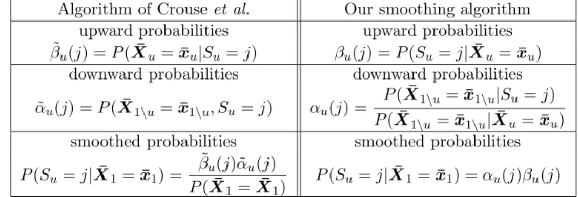
Table 1 points out the differences between theupward-downwardof Crouseet al. (1998) [6], using the decomposition of joint probabilities, and our algorithm, using the decompo-sition of the smoothed probabilities.
As for Devijver’s algorithm, the execution of the above procedure does not cause un-derflow problems. The term that dominates the recursion complexity for the computation of the hidden state distributions is 2nK2. The complexities of ourupward anddownward
recursions also have dominant term 2nK2 for binary trees (or for any tree such as the
degree of each node remains bounded). Thus, the complexity of the upward-downward
algorithm using smoothed probabilities remains inO(nK2), as the algorithm of Crouseet al. (1998), but with the complexity increasing by 50%.
Table 1: Differences between the upward-downward algorithm of Crouse et al. (1998) and our smoothing upward-downward algorithm
Algorithm of Crouseet al. Our smoothing algorithm upward probabilities upward probabilities ˜
βu(j) =P(X¯u=x¯u|Su =j) βu(j) =P(Su =j|X¯u =x¯u)
downward probabilities downward probabilities ˜
αu(j) =P(X¯1\u =x¯1\u, Su =j) αu(j) =
P(X¯1\u=x¯1\u|Su =j)
P(X¯1\u=x¯1\u|X¯u=x¯u) smoothed probabilities smoothed probabilities
P(Su =j|X¯1 =x¯1) =
˜
βu(j)˜αu(j)
P(X¯1=X¯1) P(Su =j|X¯1 =x¯1) =αu(j)βu(j)
4
Viterbi algorithm
Given an observed tree x¯1, our aim is to find the hidden state tree s¯∗
1 = (s∗1, . . . , s∗n)
maximizing P(S¯1 = ¯s1|X¯1 =x¯1) – or, equivalently, P(S¯1 =s¯1,X¯1 =x¯1), see Rabiner (1989) [18] – and the valueP∗of the maximum. We call any algorithm solving this problem
a Viterbi algorithm in reference to the hidden Markov chain terminology.
The initial global restoration algorithm for nonindependent mixture models is due to Viterbi. The Viterbi algorithm is originally intended for the analysis of Markov processes observed in memoryless noise. In the case of a hidden Markov chain{St, Xt;t= 0,1, . . .},
let Sn1 = sn1 denote the state sequence of length n and Xn1 = xn1 denote the output sequence of length n. The Viterbi algorithm for hidden Markov chains is basically a forward recursion computing the quantities
˜
δt(j) = max s1,...,st−1
P(St=j,St1−1=s1t−1,Xt1 =xt1), (8)
starting at the initial stateS1.
A natural adaptation of the Viterbi algorithm to HMT models would involve a down-ward recursion starting at the root state S1. We claim that this is not possible, for the
same reason as for our smoothing algorithm, namely, that thedownward recursion would require the results of theupward recursion (see section 3). Thus, we need to design a new Viterbi algorithm for hidden Markov chains based on a backward recursion, which will be the basis of our adaptation to HMT models.
decompo-sition, adaptated from Jelinek (1997) [13] max s1,...,sn P(Sn1 =sn1,Xn1 =xn1) = max st { max st+1,...,sn P(Xn t =xnt,Snt+1 =snt+1|St=st) × max s1,...,st−1 P(St1=st1,Xt−1 1 =xt1−1)}. (9) Let us define δt(j) = max st+1,...,sn P(Xn t =xnt,Snt+1 =snt+1|St=j).
Decomposition (9) can then be rewritten as max s1,...,sn P(Sn 1 =sn1,Xn1 =xn1) = max j {δt(j) maxs1,...,st−1 P(St=j,St1−1 =s1t−1,Xt1−1=xt1−1)}.
Using the quantities δt(j), we can build a Viterbi algorithm for hidden Markov chains
based on a backward recursion, which is equivalent to that of Brushe et al. (1998) [3]. This is initialized fort=n by
δn(j) = P(Xn=xn|Sn=j)
= Pθj(xn).
The backward recursion is given, fort=n−1, . . . ,1, by
δt(j) = max st+1,...,sn P(Xn t =xnt,Snt+1=snt+1|St=j) = max k {st+2max,...,sn P(Xnt+1 =xn t+1,Snt+2=snt+2|St+1=k) ×P(St+1 =k|St=j)}P(Xt=xt|St=j) = max k {δt+1(k)pjk}Pθj(xt).
We obtain, fort= 1,δ1(j) = max
s2,...,sn
P(Xn
1 =xn1,Sn2 =sn2|S1 =j). Hence, the probability
of the optimal state sequence associated with the observed sequencexn
1 is P∗ = max j {smax2,...,sn P(Xn1 =xn1,Sn2 =sn2|S1 =j)P(S1 =j)} = max j {δ1(j)πj}.
Transposing decomposition (9) to hidden Markov tree models yields for allu
max ¯ s1 P(S¯1=s¯1,X¯1 =x¯1) = max su {max ¯ s c(u) P(X¯u =x¯u,S¯c(u) =s¯c(u)|Su =su) ×max ¯ s1\u P(S¯1\c(u)=¯s1\c(u),X¯1\u =x¯1\u)}. (10)
Let us define δu(j) = max ¯ s c(u) P(X¯u=x¯u,S¯c(u)=s¯c(u)|Su =j) (11) δρ(u),u(j) = max ¯ su P(X¯u=x¯u,S¯u =s¯u|Sρ(u)=j). (12)
Hence (10) can be rewritten as max ¯ s1 P(S¯1 =s¯1,X¯1=x¯1) = max j δu(j) max ¯ s1\ u P(Su=j,S¯1\u =¯s1\u,X¯1\u=x¯1\u) .
The main change with respect to hidden Markov chains is that it is not possible to design a downward recursion on the basis of this type of decomposition but solely an upward recursion.
The Viterbi algorithm for a hidden Markov tree is initialized for each leaf by
δu(j) = P(Xu =xu|Su =j)
= Pθj(xu).
Then, for each of the remaining nodes taken upwards, we have the following recursion
δu(j) = max ¯ s c(u) P(X¯u =x¯u,S¯c(u) =¯sc(u)|Su=j) = ( Q v∈c(u) max ¯ sv P(X¯v =x¯v,S¯v =s¯v|Su=j) ) P(Xu =xu|Su =j) = ( Q v∈c(u) δu,v(j) ) Pθj(xu); δρ(u),u(j) = max ¯ su P(X¯u =x¯u,S¯u =s¯u|Sρ(u) =j) = max k max ¯ s c(u) P(X¯u =x¯u,S¯c(u) =¯sc(u)|Su=k)P(Su =k|Sρ(u) =j) = max k {δu(k)pjk}.
The probability of the optimal state tree associated with the observed treex¯1 is
P∗ = max
j {δ1(j)πj}.
The Viterbi algorithm is similar to theupward recursion of Crouseet al. (1998) [6] where the summations on the states are replaced by maximizations. Its complexity is inO(nK2),
and no normalization quantities are required. To retrieve the optimal state tree, it is necessary to store for each nodeu and each state j the optimal states corresponding to each of the children. The backtracking procedure consists in tracing downward along the backpointers from the optimal root state to the optimal leaf states.
5
Application to signal processing
In this section, we develop one example of application, illustrating the importance of the hidden Markov tree model. Let xT
1 = (x1, . . . , xT) be a realization of a sampled
piece-wise constant (H¨older) regularity process, for example a piecewise homogeneous fractional Brownian motion (H-FMB). The local regularity of a function (or of the trajectory of a stochastic process) is defined as by Mallat (1998) [15] as follows: the functionf has local regularityk < h < k+ 1, at timet, if there exists two constants 0< C <∞and 0< t0 as
well as a polynomialPk of orderk, such that for all t−t0 < l < t+t0 and for all h′ ≤h,
|f(l)−Pk(l)|< C|l−t|h
′
. (13)
In our simulation, we consider the slightly modified model of a compound-FBM. This model assumes that T = 2M and that from t = 1 to t = T
0 with 1 ≤T0 < T, the local
regularity of the process isH =H0, and from t=T0+ 1 to t=T, its local regularity is
H=H1. Our aim is not to estimateH0 orH1 but rather to determine the transition time
T0. To motivate our work, we recall for instance the article of Abry and Veitch (1998)
[1] where they show the major importance of detecting local regularity changes, in the context of network traffic analysis.
Our method is based on a multiresolution analysis of xT
1. As a first step, we compute
an orthonormal discrete wavelet transform of xT
1 through the following inner product:
(wm
n)1≤m≤J0,0≤ n≤2m−1, withwmn =
P2M
k=1xk2m/2ψ(2mk−n) andJ0 corresponding to
the finest scale.
As in Crouse, Nowak and Baraniuk (1998), we combine a statistical approach with a wavelet-based signal processing. This means that we process the signalxT
1 by operating on
its wavelet coefficients (wmn)m,n and that we consider these coefficients to be realizations
of random variables (Wnm)m,n. The authors justify a hidden Markov binary tree model for
the wavelet coefficients by two observations:
• residual dependencies remain between wavelet coefficients;
• wavelet coefficients are generally non-Gaussian.
We recall that the path of an H-FBM has local H¨older regularity H almost surely almost everywhere. Hence from Jaffard (1991) [12], Flandrin (1992) [11] and Wornell
et al. (1992) [22], the random variables Wnm of its wavelet decomposition are normally, identically distributed within scale and centered with variance
var(Wnm) =σ22m(2H+1).
In our simple test signal, where the local regularity is H0 for 1 ≤ t ≤ T0 and H1 for
T0+ 1≤t≤T, we consider a two-state model with the following conditional distributions:
(Wnm|Snm =j) ∼ N(0, σ2j2m(2Hj+1)).
Thus, we model the distribution of (wmn)m,nby the following hidden Markov tree model:
• Wm
n arises from a mixture of distributions with density
f(Wnm=wnm) = 1 X j=0 P(Snm =j)fθj(w m n)
where Snm is a discrete variable with two states, denoted{0,1}, and fθj(w
m
n) is the
Gaussian distribution density with mean 0 and variance σj22m(2Hj+1);
• (Snm)m,n is a Markov binary tree (i.e. each nonterminal node has exactly two
chil-dren) with parameters (πj)j and (pij)i,j;
• the wavelet coefficients are independent, conditionally to the hidden states. As in Section 2, we denote the observed tree (Wm
n )m,n by W¯ 1 =w¯1 and the hidden tree
(Sm
n)m,n by S¯1 =¯s1.
In the case of an abrupt regularity jump at time T0, the hidden tree model (W¯ 1,S¯1)
satisfies the following two properties:
• for each subtree S¯u of S¯1, there exists j in {0,1} such as the left subtree of S¯u is entirely in statej, or its right subtree is entirely in statej,
• if SJ0
t1 and S
J0
t2 are two leaves witht1 < t2 such as
SJ0
t1 =S
J0
t2 =j, then for all t between t1 andt2,S
J0
t =j.
To detect the local regularity jump, we compute the discrete wavelet transformwmn of the signal using a compact support Daubechies wavelet. An important proviso is that the chosen wavelet has regularity larger than the regularity of the process itself. In our case,
we are dealing withH∈(0,1); therefore we choose the simplest possible wavelet: the Haar with regularity one. Since our model assumes two states per tree, here, we need a single tree decomposition. This imposes only one wavelet coefficient at the coarsest scale (root node), and thus,T = 2J0 for fullJ
0-level tree 1. Then, we estimate the model parameters
by the EM algorithm, using ourupward-downward algorithm with smoothed probabilities to implement the E step. We could not use theupward-downward algorithm of Crouseet al. (1998) [6] directly (i.e. without an ad hoc scaling procedure) since underflow errors occur for values ofT typically greater than 128.
The Hj and σj parameters are estimated at the M step with a procedure adaptated
from the maximum likelihood estimation derived by Wornell and Oppenheim (1992) [22]. Thus, we obtain ˆP, ˆπ, ˆσ0, ˆσ1, ˆH0, and ˆH1. The jump detection is performed by a hidden
state restoration under the two constraints above, using the Viterbi algorithm. We obtain a value for the hidden treeS¯1 such as exactly one subtreeS¯u of S¯1 is in statej, andS¯1\t is in state 1−j. Thus, there is only one leave SJ0
t∗ such as StJ∗0 6=StJ∗0+1. The jump time T0 is estimated by:
ˆ
T0= 2.t∗.
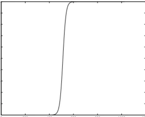
In practice, to avoid a too-severe discontinuity in the path at the transition timeT0and
to ensure that at any pointt, the local regularity H(t) is correctly defined, we synthesize a multifractional Brownian motion as proposed and defined in L´evy V´ehel and Peltier (1995) [17], with a continuous transitional H¨older regularity (Figure 3):
∀t∈ {1, . . . ,1024} H(t) = 0.1 tanh(−20 +40(t−1)
1023 ) + 0.5. (14) We set the asymptotics H0 = 0.4 and H1 = 0.6. We then construct the process x10241 =
(x(t))t=1,...,1024 with local regularity given by (14). One realization path of such a process
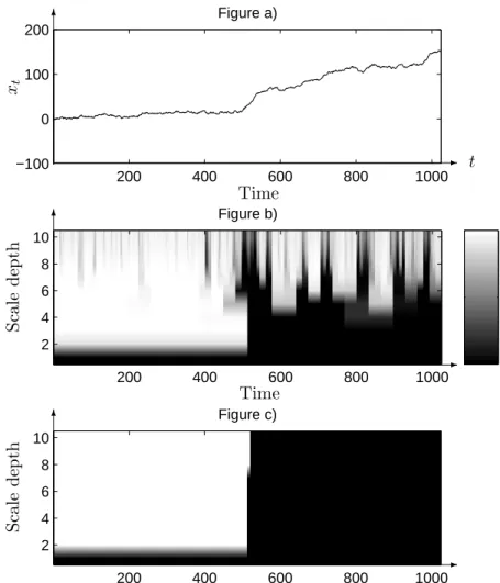
is shown in Figure 4 a).
Figure 4 b) shows the map of the smoothed probabilities P(Sm
n = 1|W¯ 1 =w¯1). We
define the depthJ(u) (or scale) of a node uas the number of nodes on the path between the root and nodeu. Our convention is that the depth of the tree root is equal to one.
1If
T is not a power of 2, we can zero-pad the series and consider a third state in the model with arbitrary small variance.
0 200 400 600 800 1000 1200 0.4 0.42 0.44 0.46 0.48 0.5 0.52 0.54 0.56 0.58 0.6
Figure 3: H¨older trajectory: Time varying local regularity.
The depth of the observed or hidden tree is defined by max
u J(u). Thus, in our case, the
depth of the tree is equal to J0. The Y-axis of the plot represents the tree depth, with
root at the bottom line. Figure 4 c) shows the result of the hidden state restoration. The border between both states is used to locate the transition timeT0inH(t). The estimated
parameters are ˆH0 = 0.3009, ˆH1 = 0.6649 and ˆT0 = 520.
These results deserve several remarks. First, the estimates ofH0andH1are imprecise,
due to the small number of time-samples for each state. Nonetheless, they are coherent with the performances discussed in Wornell and Oppenheim (1992) [22]. In particular, the method used for the estimation of Hj and σj suffers from the same limitations as the
algorithm described in Wornell and Oppenheim. On the other hand, and as far as the discrimination is concerned, the separation of the mixture components achieved by our method is very accurate. Most importantly, thanks to the restoration procedure, loose estimates forH do not affect the transition time determination ˆT0.
In a perspective viewpoint, to improve the estimates, we could substitute likelihood maximization with alternative methods. For instance, to derive estimates of the param-eters H0 and H1, it is possible to use a (weighted) linear regression of the within-scale
empirical variance, restricted to a more relevant scale sub-range.
In our elementary example, the smoothed probability map (Figure 4-b) is merely a complementary stage to restoration. Yet, let us comment on the apparent uncertainty of the states observed after transition time T0. Recalling the definition of the local H¨older
regularity of a given path, h is the supremum over all h′ satisfying inequality in (13).
0 0.5 1 Figure b) 200 400 600 800 1000 2 4 6 8 10 200 400 600 800 1000 −100 0 100 200 Figure a) Figure c) 200 400 600 800 1000 2 4 6 8 10 Time t xt -6 Time S ca le d ep th -6 Time S ca le d ep th -6
Figure 4: Hidden tree associated with a wavelet decomposition of a signal – a) A path of a piecewise-constant FBM with regularity H0 = 0.4 (corresponding to state 0) for t=
1, . . . ,512 and regularity H1 = 0.6 (corresponding to state 1) for t = 513, . . . ,1024. b) Map of the smoothed probabilities. The grey level indicates the value of the conditional probability of state 1 occurrence at a given node. c) Restored hidden tree.
analyzing the more regular part of the trace, the retained two-state model actually allows for estimating local regularities smaller than the effective one, hence, these changeovers. Again, in accordance with definition (13), this clearly does not happen with the left-hand side of the path (less regular part).
More interestingly, now, a probabilistic map becomes fully interesting on its own, when exploring more complex situations. To support our claim, let us elaborate on two examples.
• We return to our previous two-state example and assume a smooth transition from
values within interval [H0, H1], turning the frontier between the two stable states very
fuzzy. A binary segmentation obtained with the restoration algorithm may not be so sensible and necessarily implies some arbitrariness in selecting the transition timeT0.
Instead, the probabilistic map, which is output of the smoothing algorithm, provides us with afuzzy segmentationthat conveys more valuable information concerning the dynamics of the transition.
• The second example concerns situations referred to as multifractals; see, e.g., Riedi (2000) [19]. In short, for such processes, local H¨older regularity H is itself a ran-dom variable leading to utterly erratic H¨older paths (t, H(t)) and whose pointwise estimation becomes totally unrealistic. Instead, we resort to the notion of singular-ity spectrum that allows for quantifying how frequently a given singularsingular-ity strength
H(t) = h is assumed. Then, probabilistic maps, like the one displayed in figure 4-b, can easily be thought as a measure of occurrence of the quantized regularity
hk, k= 1, . . . , K associated with the given statek. Conceptually, it would suffice to
marginalize these distributions and to represent the obtained a priori probabilities
Pk versushk, to get a discrete singularity density(hk, Pk).
Another very interesting extension of hidden Markov tree models is to consider, as for hidden Markov chains, continuous-valued hidden states. It is known that the estimation problem in such models is difficult. However, from an application viewpoint and when the model is entirely specified, it would allow for modeling signals with continuously time varying local regularity. In this context, it would be possible to compute the local regularity distribution conditionally to the observed wavelet coefficients.
6
Concluding remarks
In this paper, we developed a smoothing algorithm, which implements the E step of the EM algorithm for parameter estimation. The important improvement carried out to the existing algorithm of Crouseet al. (1998) [6] is that ours is not subject to underflow. This allows us to apply hidden Markov trees to large data sets.
Another important innovation of our methodology is the use of the smoothed proba-bility map. In particular, we showed it to be relevant in a wavelet-tree application and,
in possible extensions, to models with continuous-valued hidden states.
As this application demonstrates the need for a global restoration algorithm, a solution based on the adaptation of a backward Viterbi algorithm for hidden Markov chains has been proposed.
Acknowledgments
The authors acknowledge helpful advice and discussion about inference algorithms in mix-ture models with Gilles Celeux. They are thankful to the anonymous reviewers for their useful comments.
References
[1] P. Abry and D. Veitch. Wavelet Analysis of Long Range Dependant Traffic. IEEE Transactions on Information Theory, 44(1):2–15, January 1998.
[2] L.E. Baum, T. Petrie, G. Soules, and N. Weiss. A Maximization Technique Occurring in the Statistical Analysis of Probabilistic Functions of Markov Chains. The Annals of Mathematical Statistics, 41(1):164–171, 1970.
[3] G.D. Brushe, R.E. Mahony, and J.B. Moore. A Soft Output Hybrid Algorithm for ML/MAP Sequence Estimation. IEEE Transactions on Information Theory, 44(7):3129–3134, November 1998.
[4] H. Choi and R.G. Baraniuk. Multiscale Image Segmentation using Wavelet-Domain Hidden Markov Models. IEEE Transactions on Image Processing , to be published in 2001.
[5] G.A. Churchill. Stochastic Models for Heterogeneous DNA Sequences. Bulletin of Mathematical Biology, 51:79–94, 1989.
[6] M.S. Crouse, R.D. Nowak, and R.G. Baraniuk. Wavelet-Based Statistical Signal Processing Using Hidden Markov Models. IEEE Transactions on Signal Processing, 46(4):886–902, April 1998.
[7] N. Dasgputa, P. Runkle, L. Couchman, and L. Carin. Dual hidden Markov model for characterizing wavelet coefficients from multi-aspect scattering data. Signal Process-ing, 81(6):1303–1316, 2001.
[8] P. A. Devijver. Baum’s forward-backward Algorithm Revisited. Pattern Recognition Letters, 3:369–373, 1985.
[9] M. Diligenti, P. Frasconi, and M. Gori. Image Document Categorization using Hidden Tree Markov Models and Structured Representations. In S. Singh, N. Murshed, and W. Kropatsch, editors, Second International Conference on Advances in Pattern Recognition. Lecture Notes in Computer Science, 2001.
[10] Y. Ephraim and N. Merhav. Hidden Markov processes.IEEE Transactions on Infor-mation Theory, 48:1518–1569, June 2002.
[11] P. Flandrin. Wavelet Analysis and Synthesis of Fractional Brownian Motion. IEEE Transactions on Information Theory, 38:910–917, 1992.
[12] S. Jaffard. Pointwise Smoothness, two-microlocalization and Wavelet Coefficients.
Publications Math´ematiques, 35:155–168, 1991.
[13] F. Jelinek. Statistical Methods for Speech Recognition. MIT Press, 1997.
[14] S.E. Levinson, L.R. Rabiner, and M.M. Sondhi. An Introduction to the Application of the Theory of Probabilistic Functions of a Markov Process in Automatic Speech Recognition. Bell System Technical Journal, 62:1035–1074, 1983.
[15] S. Mallat. A Wavelet Tour of Signal Processing. San Diego, California: Academic Press. xxiv, 1998.
[16] G. McLachlan and T. Krishnan. The EM Algorithm and Extensions. J. Wiley and sons, 1997.
[17] R. Peltier and J. Levy-Vehel. Multifractional Brownian Motion : Definition and Pre-liminary Results. Technical Report RR-2645, INRIA, 1995. Submitted to Stochastic Processes and their Applications.
[18] L.R. Rabiner. A Tutorial on Hidden Markov Models and Selected Applications in Speech Recognition. InProceedings of the IEEE, volume 77, pages 257–286, February 1989.
[19] R. Riedi. Long range dependence : theory and applications, chapter Multifractal processes. Boston, MA: Birkhauser, 2000. Also Technical Report, ECE Dept. Rice Univ., TR 99-06.
[20] O. Ronen, J.R. Rohlicek, and M. Ostendorf. Parameter Estimation of Dependance Tree Models Using the EM Algorithm. IEEE Signal Processing Letters, 2(8):157–159, August 1995.
[21] P. Smyth, D. Heckerman, and M.I. Jordan. Probabilistic Independence Networks for Hidden Markov Probability Models. Neural Computation, 9(2):227–270, 1997. [22] G.W. Wornell and A.V. Oppenheim. Estimation of Fractal Signals from Noisy
Mea-surements Using Wavelets. IEEE Transactions on Signal Processing, 40(3):611–623, March 1992.
![Table 1 points out the differences between the upward-downward of Crouse et al. (1998) [6], using the decomposition of joint probabilities, and our algorithm, using the decompo-sition of the smoothed probabilities.](https://thumb-us.123doks.com/thumbv2/123dok_us/776174.2598140/13.918.210.763.290.521/differences-downward-crouse-decomposition-probabilities-algorithm-smoothed-probabilities.webp)