Introduction to Various Algorithms of Speech Recognition: Hidden Markov Model, Dynamic Time Warping and Artificial Neural Networks

(1)

IJEDR1404035

International Journal of Engineering Development and Research (www.ijedr.org)

3590

Introduction to Various Algorithms of Speech

Recognition: Hidden Markov Model, Dynamic Time

Warping and Artificial Neural Networks

Pahini A. Trivedi

V.V.P. Engineering College

Rajkot, Gujarat, India

Abstract - Now a day’s speech recognition is used widely in many applications. In computer science and electrical engineering, speech recognition (SR) is the translation of spoken words into text. It is also known as "automatic speech recognition" (ASR), "computer speech recognition", or just "speech to text" (STT). A hidden Markov model (HMM) is a statisticalMarkov model in which the system being modelled is assumed to be a Markov process with unobserved (hidden) states. An HMM can be presented as the simplest dynamic Bayesian network. Dynamic time warping (DTW) is a well-known technique to find an optimal alignment between two given (time-dependent) sequences under certain restrictions intuitively; the sequences are warped in a nonlinear fashion to match each other. ANN is non-linear data driven self-adaptive approach. It can identify and learn co-related patterns between input dataset and corresponding target values. After training ANN can be used to predict the outcome of new independent input data.

Index Terms - SR, HMM, DTW, ANN

I.INTRODUCTION

In computer science and electrical engineering, speech recognition (SR) is the translation of spoken words into text. It is also known as "automatic speech recognition" (ASR), "computer speech recognition", or just "speech to text" (STT).

Some SR systems use "speaker-independent speech recognition while others use "training" where an individual speaker reads sections of text into the SR system. These systems analyse the person's specific voice and use it to fine-tune the recognition of that person's speech, resulting in more accurate transcription. Systems that do not use training are called "speaker-independent" systems. Systems that use training are called "speaker-dependent" systems. [1]

Designing a machine that mimics human behaviour, particularly the capability of speaking naturally and responding properly to spoken language, has intrigued engineers and scientists for centuries. Since the 1930s, when Homer Dudley of Bell Laboratories proposed a system model for speech analysis and synthesis [3, 4]. The first speech recognizer appeared in 1952 and consisted of a device for the recognition of single spoken digits [5] another early device was the IBM Shoebox, exhibited at the 1964 New York World's Fair. Lately there have been numerous improvements like a high speed mass transcription capability on a single system like Sonic Extractor [5] One of the most notable domains for the commercial application of speech recognition in the United States has been health care and in particular the work of the medical transcriptionist (MT). [2]

The performance of speech recognition systems is usually evaluated in terms of accuracy and speed. Accuracy is usually rated with word error rate (WER), whereas speed is measured with the real time factor. Other measures of accuracy include Single Word Error Rate (SWER) and Command Success Rate (CSR). [6]

However, speech recognition (by a machine) is a very complex problem. Vocalizations vary in terms of accent, pronunciation, articulation, roughness, nasality, pitch, volume, and speed. Speech is distorted by a background noise and echoes, electrical characteristics. Accuracy of speech recognition varies with the following: [7] [1]

 Vocabulary size and confusability  Speaker dependence vs. independence  Isolated, discontinuous, or continuous speech  Task and language constraints

 Read vs. spontaneous speech  Adverse conditions

A. Application of Speech Recognition[1]  Hands-free computing

 Home automation  Interactive voice response

(2)

IJEDR1404035

3591

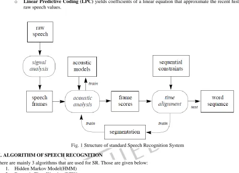
B. Structure of standard Speech Recognition System

The structure of a standard speech recognition system is illustrated in Figure 2. The elements are as follows:

 Raw speech. Speech is typically sampled at a high frequency, e.g., 16 KHz over a microphone or 8 KHz over a telephone. This yields a sequence of amplitude values over time.

 Signal analysis. Raw speech should be initially transformed and compressed, in order to simplify subsequent processing. Many signal analysis techniques are available which can extract useful features and compress the data by a factor of ten without losing any important information. Among the most popular:

o Fourier analysis (FFT) yields discrete frequencies over time, which can be interpreted visually. Frequencies are often distributed using a Mel scale, which is linear in the low range but logarithmic in the high range, corresponding to physiological characteristics of the human ear.

o Perceptual Linear Prediction (PLP) is also physiologically motivated, but yields coefficients that cannot be interpreted visually.

o Linear Predictive Coding (LPC) yields coefficients of a linear equation that approximate the recent history of the raw speech values.

Fig. 1 Structure of standard Speech Recognition System

II.ALGORITHMOFSPEECHRECOGNITION

There are mainly 3 algorithms that are used for SR. Those are given below: 1. Hidden Markov Model(HMM)

2. Dynamic Time Warping(DTW) 3. Artificial Neural Networks(ANN)

Above algorithms are explained in detail in further sections.

III.HIDDENMARKOVMODEL(HMM)

(3)

IJEDR1404035

3592

Fig. 2 A simple Hidden Markov Model, with two states and two output symbols, A and B.

HMMs have a variety of applications. When an HMM is applied to speech recognition, the states are interpreted as acoustic models, indicating what sounds are likely to be heard during their corresponding segments of speech; while the transitions provide temporal constraints, indicating how the states may follow each other in sequence. Because speech always goes forward in time, transitions in a speech application always go forward. [5]

A. Algorithms of HMM

There are three basic algorithms associated with Hidden Markov Models:  Forward algorithm, useful for isolated word recognition;  Viterbi algorithm, useful for continuous speech recognition; and  Forward-backward algorithm, useful for training an HMM.

B. Limitations of HMM

 Constant observation of frames  The Markov assumption

 Lack of formal methods for choosing a model topology  Large amounts of training data required

 Weak duration modelling  Restricted output PDFs

 The assumption of conditional independence

IV.DYNAMICTIMEWARPING(DTW)

The simplest way to recognize an isolated word sample is to compare it against a number of stored word templates and determine which the “best match” is. This goal is complicated by a number of factors. First, different samples of a given word will have somewhat different durations. This problem can be eliminated by simply normalizing the templates and the unknown speech so that they all have an equal duration. However, another problem is that the rate of speech may not be constant throughout the word; in other words, the optimal alignment between a template and the speech sample may be nonlinear. Dynamic Time Warping (DTW) is an efficient method for finding this optimal nonlinear alignment.

Dynamic time warping (DTW) is a well-known technique to find an optimal alignment between two given (time-dependent) sequences under certain restrictions intuitively; the sequences are warped in a nonlinear fashion to match each other. Originally, DTW has been used to compare different Speech patterns in automatic speech recognition. In fields such as data mining and information retrieval, DTW has been successfully applied to automatically cope with time deformations and different speeds associated with time-dependent data.

In time series analysis, dynamic time warping (DTW) is an algorithm for measuring similarity between two temporal sequences which may vary in time or speed. For instance, similarities in walking patterns could be detected using DTW, even if one person was walking faster than the other can also detected by DTW.

Problem of finding an average sequence for a set of sequences. The average sequence is the sequence that minimizes the sum of the squares to the set of objects. [5]

V.ARTIFICIALNEURALNETWORKS(ANN)

A neural network can be defined as a model of reasoning based on the human brain. The brain consists of a densely interconnected set of nerve cells, or basic information-processing units, called neurons. The human brain incorporates nearly 10 billion neurons and 60 trillion connections, synapses, between them. By using multiple neurons simultaneously, the brain can perform its functions much faster than the fastest computers in existence today.

(4)

IJEDR1404035

3593

Fig. 3 Biological Neural Network

An artificial neural network consists of a number of very simple processors, also called neurons, which are analogous to the biological neurons in the brain. The neurons are connected by weighted links passing signals from one neuron to another. The output signal is transmitted through the neuron’s outgoing connection. The outgoing connection splits into a number of branches that transmit the same signal. The outgoing branches terminate at the incoming connections of other neurons in the network.

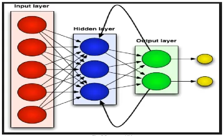
Fig. 4 Architecture of ANN

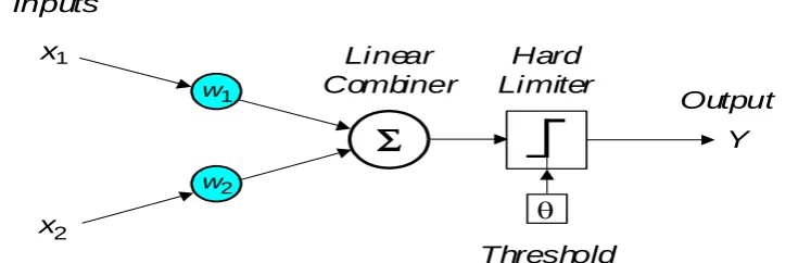
The perceptron is the simplest form of a neural network. It consists of a single neuron with adjustable synaptic weights and a hard limiter. The operation of Rosenblatt’s perceptron is based on the McCulloch and Pitts neuron model. The model consists of a linear combiner followed by a hard limiter.

Fig. 5 Single layer two input perceptron A. Learning in ANN

There are basically three types of learning, 1. Supervised Learning

2. Un- Supervised Learning 3. Reinforced Learning

 Supervised Learning - Applications in which the training data comprises examples of the input vectors along with their corresponding target vectors (output vectors) are known as supervised learning problems.Supervised learning is when the data you feed your algorithm is "tagged" to help your logic make decisions. Eg. Face recognition, perceptron

 Un- Supervised Learning - In other pattern recognition problems, the training data consists of a set of input vectors x without any corresponding target values. The goal in such unsupervised learning problems may be to discover groups of similar examples within the data, where it is called clustering.Clustering is unsupervised learning: you let the algorithm decide how to group samples into classes that share common properties. Eg. Hopfield Network

Soma _Soma

Synapse

Dendrites

Axon

Synapse Dendrites

Axon

Input Layer Output Layer Middle Layer

Threshold

Inputs

x

1

x

₂

Output

Y

Hard

Limiter

w₂

w₁

Linear

Combiner

(5)

IJEDR1404035

3594

 Reinforced Learning - In reinforcement learning, data are usually not given, but generated by an agent's interactions with

the environment. At each point in time , the agent performs an action and the environment generates an observation and an instantaneous cost , according to some (usually unknown) dynamics. The aim is to discover a policy for selecting actions that minimizes some measure of a long-term cost; i.e., the expected cumulative cost. The environment's dynamics and the long-term cost for each policy are usually unknown, but can be estimated.[8]

B. Types of ANN There are two types of ANN,

1. Feed-Forward NN 2. Recurrent NN

 Feed-Forward Neural Network(FFNN) - A feed forward neural network is an artificial neural network where connections between the units do not form directed.

(6)

IJEDR1404035

3595

 Recurrent NN - A recurrent neural network (RNN) is a class of artificial neural network where connections between units

form a directed cycle. This creates an internal state of the network which allows it to exhibit dynamic temporal behaviour.

Fig. 7 Recurrent NN C. Advantages of ANN

 ANNs are highly non-linear modelling

 ANN is nonlinear model that is easy to use and understand compared to statistical methods.

 ANN is non-parametric model while most of statistical methods are parametric model that need higher background of statistic.

 ANN with Back propagation (BP) learning algorithm is widely used in solving various classifications and forecasting problems. Even though BP convergence is slow but it is guaranteed.[9]

 Neural networks offer a number of advantages, including requiring less formal statistical training, ability to implicitly detect complex nonlinear relationships between dependent and independent variables, ability to detect all possible interactions between predictor variables, and the availability of multiple training algorithms. [10]

D. Applications of ANN  Character Recognition  Image Compression  Stock Market Prediction  Travelling Salesman Problem  Medicine and Security

VI.CONCLUSION

For SR ANN is a effective and efficient way as it has multi layer network. Speech Recognition is also used in smart phones. In smart phones speech/spoken words are given as an input and SR s/w gives appropriate search or information that user wants as a output.Neural networks, with their remarkable ability to derive meaning from complicated or imprecise data, can be used to extract patterns and detect trends that are too complex to be noticed by either humans or other computer techniques. A trained neural network can be thought of as an "expert" in the category of information it has been given to analyse. ANN has,

1. Adaptive learning: An ability to learn how to do tasks based on the data given for training or initial experience.

2. Self-Organisation: An ANN can create its own organisation or representation of the information it receives during learning time.

3. Real Time Operation: ANN computations may be carried out in parallel, and special hardware devices are being designed and manufactured which take advantage of this capability.

(7)

IJEDR1404035

3596

REFERENCES

[1] http://en.wikipedia.org/wiki/Speech_recognition.

[2] B.H. Juang & Lawrence R. Rabiner, “Automatic Speech Recognition – A Brief History of the Technology Development "Georgia Institute of Technology, Atlanta, Rutgers University and the University of California, Santa Barbara.

[3] H. Dudley, the Vocoder, Bell Labs Record, Vol. 17, pp. 122-126, 1939.

[4] H. Dudley, R. R. Riesz, and S. A. Watkins, A Synthetic Speaker, J. Franklin Institute, Vol. 227, pp. 739-764, 1939.

[5] Joe Tebelskis, ''Speech Recognition using Neural Networks'', May 1995, CMU-CS-95-142, School of Computer Science, Carnegie Mellon University Pittsburgh, Pennsylvania 15213-3890.

[6] Deng Y. , Li X. , Kwan C.,Raj B.,Stern R., ''Continuous Feature Adaptation for Non-Native Speech Recognition'', International Journal of Computer, Information Science and Engineering ,Vol:1 No:6, 2007.

[7] National Institute of Standards and Technology, ''The History of Automatic Speech Recognition Evaluation'', at NIST. [8] http://en.wikipedia.org/wiki/Artificial_neural_network