R E S E A R C H
Open Access
Ensemble hidden Markov models with
application to landmine detection
Anis Hamdi and Hichem Frigui
*Abstract
We introduce an ensemble learning method for temporal data that uses a mixture of hidden Markov models (HMM). We hypothesize that the data are generated by K models, each of which reflects a particular trend in the data. The proposed approach, called ensemble HMM (eHMM), is based on clustering within the log-likelihood space and has two main steps. First, one HMM is fit to each of the N individual training sequences. For each fitted model, we evaluate the log-likelihood of each sequence. This results in an N-by-N log-likelihood distance matrix that will be partitioned into K groups using a relational clustering algorithm. In the second step, we learn the parameters of one HMM per cluster. We propose using and optimizing various training approaches for the different K groups depending on their size and homogeneity. In particular, we investigate the maximum likelihood (ML), the minimum classification error (MCE), and the variational Bayesian (VB) training approaches. Finally, to test a new sequence, its likelihood is computed in all the models and a final confidence value is assigned by combining the models’ outputs using an artificial neural network. We propose both discrete and continuous versions of the eHMM.
Our approach was evaluated on a real-world application for landmine detection using ground-penetrating radar (GPR). Results show that both the continuous and discrete eHMM can identify meaningful and coherent HMM mixture components that describe different properties of the data. Each HMM mixture component models a group of data that share common attributes. These attributes are reflected in the mixture model’s parameters. The results indicate that the proposed method outperforms the baseline HMM that uses one model for each class in the data.
Keywords: Hidden Markov models; Mixture models; Landmine detection; Ground-penetrating radar; Clustering
1 Introduction
Detection and removal of buried landmines is a worldwide humanitarian and military problem. The latest statistics [1] show that in 2012, a total of 3618 casualties from mines were recorded in 62 countries, the vast majority (78 %) of casualties were civilians. Detection and removal of land-mines is therefore a significant problem and in recent years has attracted several researchers. One challenge in landmine detection lies in plastic or low metal mines that are difficult to detect by traditional metal detectors. Varieties of sensors have been proposed or are under investigation for landmine detection. Ground-penetrating radar (GPR) offers the promise of detecting landmines with little or no metal content. Unfortunately, landmine detection via GPR has proven to be a difficult problem
*Correspondence: [email protected]
Department of Computer Engineering and Computer Science, University of Louisville, 40292 Louisville, KY, USA
[2, 3]. Although systems can achieve high detection rates, they have done so at the expense of high false alarm rates. The key challenge to mine detection technology lies in achieving a high rate of mine detection while maintaining a low false alarm rate. The performance of a mine detec-tion system is therefore commonly measured by a receiver operating characteristics (ROC) curve that specifies the rate of true detection versus the rate of false alarm.
To improve the overall ROC of the landmine detection system, several algorithms have been introduced in the last decade. These algorithms use methods such as fuzzy logic [4], hidden Markov models [5–7], nearest neighbor classifiers [8, 9], support vector machines [10], or random forest [11] to assign a confidence that a mine is present at a point.
In [5, 6], hidden Markov modeling was proposed for detecting both metal and nonmetal mine types using data collected by a moving vehicle-mounted GPR sys-tem. These initial applications have proved that HMM
techniques are feasible and effective for landmine detec-tion. The initial work relied on simple gradient edge features. Subsequent work used an edge histogram descriptor (EHD) approach to extract features from the original GPR signatures. The baseline HMM classifier consists of two HMM models, one for mine and one for background. The mine (background) model captures the characteristics of the mine (background) signatures. The model initialization and subsequent training are based on global averaging over the training data corresponding to each class.
Most subsequent published works in the area of land-mine detection using HMMs focused on feature-level fusion [12] and/or model-level fusion [13–15]. All of these methods still use a single model for each class. In this paper, we argue that a single model is not sufficient to capture the intra-class variability. In the context of land-mine detection, variations in the class of land-mines may be caused by the different mine types, burial depth, soil type, and moisture. Similarly, background signatures may exhibit large variations due to different soil conditions and data preprocessing techniques. To generalize the HMM approach, we identify the variations within each class in an unsupervised manner and use multiple models to account for the intra-class variations.
The proposed approach consists of the construction of a mixture of HMMs to cover the diversity of the training data. This approach, called ensemble of hidden Markov models (eHMM), has four main components: similarity matrix computation, relational clustering, adaptive train-ing scheme, and decision level fusion. These components are summarized by the block diagram in Fig. 1 and will be described in section 4.
The remainder of this paper is organized as fol-lows. Section 2 provides background material on hidden Markov models. Section 3 highlights the motivations for adopting multiple models in our approach. Section 4 out-lines the eHMM architecture and describes its different components. Section 5 reports the experimental results of our eHMM approach on large GPR collections and com-pare them to those of the baseline HMM detector. Finally, conclusions are provided in Section 6.
2 Background
2.1 Hidden Markov models
An HMM is a model of a doubly stochastic process that produces a sequence of random observation vectors at discrete times according to an underlying Markov chain. At each observation time, the Markov chain may be in one ofNstates{s1,. . .,sN}and, given that the chain is in a cer-tain state, there are probabilities of moving to other states. These probabilities are called transition probabilities. Let T be the length of the observation sequence (i.e., number of time steps), let O = {O1,. . .,OT} be the observation
sequence, and letQ= {q1,. . .,qT}be the state sequence. The compact notation
λ=(A,B,π) (1)
is generally used to indicate the complete parameter set of the HMM model. In (1),A =[aij] is the state transition probability matrix, whereaij = Pr(qt = j|qt−1 = i)for i,j = 1,. . .,N; π =[πi], where πi = Pr(q1 = si) are the initial state probabilities; andB=bi(Ot),i=1,. . .,N, where bi(Ot) = Pr(Ot|qt = i) is the observation probability distribution in statei.
An HMM is called continuous if the observation prob-ability density functions are continuous and discrete oth-erwise. In the case of the discrete HMM, the observation vectors are commonly quantized into a finite set of sym-bols, {v1,v2,. . .,vM}, called the codebook. Each state is represented by a discrete probability density function and each symbol has an associated probability of occurring given that the system is in a given state. In other words, B becomes a simple set of fixed probabilities for each state. That is,bi(Ot) = bi(k) = Pr(vk|qt = i), wherevk is the nearest codebook symbol toOt.
Given the form of the hidden Markov model defined in (1), Rabiner [16] defines three key problems of interest that must be solved for the model to be useful in real-world applications: (i) the classification problem; (ii) the problem of finding an optimal state sequence; and (iii) the problem of estimating the model parameters.
The classification problem involves computing the probability of an observation sequence O = {O1, O2,. . .,OT}given a modelλ, i.e,Pr(O|λ). This probabil-ity is computed efficiently using the forward–backward procedure [16].
In most applications, it often turns out that computing an optimal state sequence is more useful than Pr(O|λ). There are several possible optimality criteria. One that is particularly useful is to maximizePr(O,Q|λ) over all possible state sequencesQ. The Viterbi algorithm [17] is an efficient and formal technique for finding this optimal state sequence and its probability.
The third problem in building an HMM is the train-ing problem: how does one estimate the parameters of the model? The problem is difficult because there are several levels of estimation required in an HMM. First, the states themselves must be estimated. Then, the model parame-tersλ = (A,B,π)need to be estimated. For the discrete HMM, first the codebook is determined, usually using the K-means algorithm [18], or other vector quantization algorithms. Then, the parameters(A,B,π)are estimated iteratively using the Baum-Welch learning algorithm [19].
Fig. 1Block diagram of the proposed eHMM
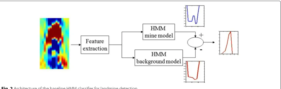
HMM models, one for mines and one for the background. Each model has four states and produces a probability value by backtracking through model states using the Viterbi algorithm [17]. The mine model,λm, is designed to capture the spatial distribution of the features. This model assumes that mine signatures have a hyperbolic shape comprised of a succession of rising, horizontal, and falling edges with variable duration in each state. The beginning and the end of the observation vectors correspond typi-cally to a non-edge (or background) state. The background model,λb, is needed to capture the background and clut-ter characclut-teristics. No prior information or assumptions are used for this model.
The architecture of the baseline HMM classifier is shown in Fig. 2. Full details of the model’s initialization and training can be found in [5]. The probability value produced by the mine (background) model can be thought of as an estimate of the probability of the observation sequence given that there is a mine (background) present. The confidence value assigned to each observation sequence, Conf(O), depends on: (1) the probability
assigned by the mine model,Pr(O|λm); (2) the probability assigned by the background model,Pr(O|λc); and (3) the optimal state sequence. Thus,
Conf(O)=
maxlogPrPr((OO||λλmc)), 0
if #{st=1,t=1,· · ·,T} ≤Tmax
0 otherwise
(2)
where #{st=1,t=1,· · ·,T}corresponds to the number of observations assigned to the background state (state 1). Tmaxis defined experimentally based on the shortest mine signature. Equation (2) ensures that sequences with a large number of observations assigned to state 1 are considered non-mines.
2.3 Extensions to the baseline HMM for landmine detection
Fig. 2Architecture of the baseline HMM classifier for landmine detection
proposed. For instance, in [12, 13], the authors pro-posed the multi-stream HMM (MSHMM) that com-bines multiple sets of features. An optimal weight for each feature was learned in the training phase. In [14], maximum likelihood (ML) and minimization of classification error (MCE) learning methods were derived for the MSHMM. In [15], HMMs with stick-breaking priors (SBHMM) [20] were employed to learn the number of HMM states in the baseline HMM landmine detector. This approach relies on a variational Bayesian learning technique in lieu of standard BW training.
3 Motivations
The baseline HMM represents each class by a single model learned from all the observations within that class. The goal is to generalize from all the training data in order to classify unseen observations. However, for complex classification problems with large intra-class variations, combining observations with different charac-teristics to learn one model might lead to too much aver-aging thus, lose the discriminating characteristics of the observations.
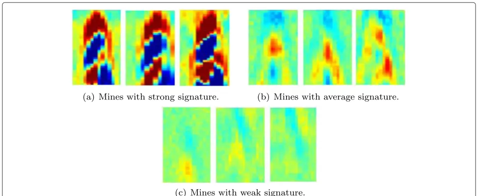
To illustrate this problem, we use the example of detect-ing buried landmines usdetect-ing GPR sensors1. In this case, the training data consists of a set ofNGPR alarms labeled as mines (class 1) or clutter (class 0). The goal is to generalize from the training data in order to classify unlabeled GPR signatures. In Fig. 3, we show three groups of mines with different signature strengths. It is obvious that grouping all of these signatures, to learn a single model, would lead to poor generalization. Similarly, the false alarms could have significant variations as they are caused by different clutter objects and varied environment conditions. These issues are more acute when data are collected by multiple sensors and/or using various features.
Consequently, learning a set of models that reflect dif-ferent characteristics of the observations might be more beneficial than using one global model for each class. This
is typical in many classifiers such as the K-NN [9], which uses different prototypes for each class, and the SVM [10], which uses multiple support vectors.
In this paper, we develop a new approach that replaces the two-model classifier with one that includes multiple models for each class. For instance, each group of signa-tures in Fig. 3 would be used to learn a different model. Our approach aims to capture the characteristics of the observations that would be lost under averaging in the two-model case.
We hypothesize that under realistic conditions, the data are generated by multiple models. The proposed approach, called ensemble HMM (eHMM), attempts to partition the training data within the log-likelihood space and identify multiple clusters in an unsupervised man-ner. Depending on each cluster’s homogeneity and size, an appropriate training scheme is applied to learn the corre-sponding HMM parameters. The resultingKHMMs are then aggregated through a decision level fusion compo-nent to form a descriptive model for the data.
4 Ensemble HMM architecture Let O = Or,yr
R
r=1 be a set of R labeled sequences of length T where Or =
O(r1),· · ·,O(rT)
Fig. 3Sample mine signatures manually categorized into three groups.aMines with strong signature.bMines with average signature.cMines with weak signature
4.1 Similarity between observations in the log-likelihood space
4.1.1 Fitting individual models to sequences
Initially, each sequence in the training data,Or, 1≤r≤R is used to learn an HMM model λr. Even though using only one sequence of observations to learn an HMM might lead to over-fitting, this technique is only an inter-mediate step that aims to capture the characteristics of each sequence. The produced HMM model is meant to give a maximal description of each sequence, and there-fore, over-fitting is not an issue in this context. In fact, it is desired that the model perfectly fits the observation sequence. In this case, the likelihood of each sequence with respect to its corresponding model is expected to be higher than those with respect to the remaining models.
Letλ(r0)
R
r=1be the set of initial models and lets
(r) n , 1≤
n ≤ N, be the representative of each state inλ(r0). Each model hasNstates. First, the model states can be assigned to the sequence observations either heuristically, using domain knowledge, or automatically by clustering the sequence observations intoN clusters. In our approach, we use the latter and we define the states’ means and observations as the center and elements of each resulting cluster, respectively. Consequently, the transition matrix and the initial probabilities ofλ(r0)are set according to the aforementioned associations. For the emission probabili-ties, the initialization differs whether we use the discrete or continuous HMM.
For the discrete case, the codewords{v1,· · ·vM}of the initial individual DHMM model are the actual observa-tions of the sequence{O1,· · ·OT}. The emission probabil-ity of each codeword in each state is inversely proportional to their distance to the mean of that state. We use
bn(m)= 1
vm−sn N
l=1vm1−sl
, 1≤m≤M, 1≤n≤N. (3)
To satisfy the requirement that Mm=1bn(m) = 1, we normalize the values using
bn(m)←− bMn(m) l=1bn(l)
, 1≤m≤M, 1≤n≤N. (4)
In the continuous case, the emission probability den-sity functions are modeled by mixtures of Gaussians. In the case of individual sequence models, as the number of observations is small, we use a single component mixture for each state. Thus, the observations belonging to each state are used to estimate the mean and covariance of that state’s component. We use
μn=mean{Ot|Ot∈sn}, 1≤n≤N, (5)
and
n=covariance{Ot|Ot∈sn}, 1≤n≤N. (6)
Then, the Baum-Welch algorithm [21] is used to adapt the model parameters to each given observation. Let{λr}Rr=1 be the set of trained individual models.
4.1.2 Log-likelihood-based similarity
The log-likelihood,L(i,j), of sequenceOibeing generated from modelλjreflects the degree to whichOifitsλjand is defined as:
L(i,j)=logPrOi|λj
. (7)
In (7),Lcan be computed using the forward–backward procedure mentioned in Section 2.1. When the log-likelihood value is high, it is likely that model λj gener-ated sequenceOi. In this case, sequencesOi andOj are expected to have common salient features and are consid-ered to be similar. On the other hand, when the likelihood term is low, it is unlikely that model λj generated the sequenceOi. In this case,OiandOjare considered to be
The likelihood-based similarity may not be always accu-rate. In fact, some observations can have high likelihood in a visually different model. This occurs when most of the elements of a sequence partially match only one or two of the states of the model. In this case, the observa-tion sequence can have a high likelihood in the model but its optimal Viterbi path will deviate from the typical path. To alleviate this problem, we introduce a penalty term, P(i,j), to the log-likelihood measure that is related to the mismatch between the most likely sequence of hidden states of the test sequence (Oi) and that of the generating sequence (Oj), i.e., Viterbi optimal path of testing sequenceOjwith modelλj, Q(jj). In (8),DEditis the “edit distance” [17] , commonly used in string comparisons. The “edit distance” between two strings, saypandq, is defined as the minimum num-ber of single-character edit operations (deletions, inser-tions, and/or replacements) that would convert p into q. The Viterbi path mismatch term is intended to ensure that similar sequences have few mismatches in their cor-responding Viterbi optimal paths. Since the Viterbi path is already available when using the forward–backward pro-cedure for the likelihood computation, the penalty term does not require significant additional computation.
Finally, we define the similarity, S, between two sequencesOiandOjby combining (7) and (8):
S(i,j)=αL(i,j)−(1−α)P(i,j). (9)
In (9), the mixing factor,α∈[ 0, 1], is a trade-off param-eter between the log-likelihood-based similarity and the
Viterbi-path-mismatch-based dissimilarity. It is estimated experimentally by maximizing the intra-class similarity and minimizing the inter-class similarity across the train-ing data. A larger value ofα corresponds to a dominant log-likelihood-based similarity where the need for the penalty mismatch is not significant. A smaller α corre-sponds to a more significant path mismatch penalty.
Using (9) to compute the similarity between all pairs of observations results in a similarity matrix that is not symmetric. Thus, we use the following three-step sym-metrization scheme to transform it into a pairwise dis-tance matrix:
The distance matrix, computed using (10), reflects the degree to which pairs of sequences are considered similar. The largest variation is expected to be between sequences from different classes. Other significant variations may exist within the same class, e.g., the groups of signatures shown in Fig. 3. Our goal is to identify the similar groups so that one model can be learned for each group. This task can be achieved using any relational clustering algo-rithm. In our work, we use the standard agglomerative hierarchical algorithm [18].
Agglomerative hierarchical clustering is a bottom–up approach that starts with each data point as a cluster. It then proceeds by merging the most similar clusters to pro-duce a sequence of clusters. Several measures have been used to assess the similarity between clusters [18]. Exam-ples include single link, complete link, average link, and ward distance. The complete link method tends to pro-duce a large number of small and compact clusters, while the single link method is known to result in few “elon-gated” clusters with large number of points. A compro-mise between the two is the minimum-variance distance, or ward distance [22]. This distance is defined as
d(i,j)= ninj ni+nj
ci−cj2 (11)
where nk andck are the cardinality and the centroid of clusterCk, respectively. It has been shown in [17] that this approach merges the two clusters that lead to the smallest increase in the overall variance.
4.3 Ensemble HMM initialization and training
class labels, clusters may include sequences from differ-ent classes. LetNk(c)be the number of sequences in cluster kthat belong to classc, such that Cc=1Nk(c) = Nk. For instance, for the landmine example, if we letc=1 denote the class of mines andc = 0 denote the class of clutter, Nk(1)would be the number of mines assigned to clusterk.
The next step of our approach consists of learning a set of HMMs that reflect the diversity of the training data. Since a cluster contains a set of similar sequences, and each cluster may include observations from different classes, we learn one HMM model
r=1 be the set of sequences partitioned into
clusterkthat belong to classcand let
For each cluster, we devise one of the following opti-mized training methods based on the cluster’s size and homogeneity.
• Clusters dominated by sequences from only one class:In this case, we learn only one model for this cluster. The sequences within this cluster are presumably similar and belong to the same ground truth class, denotedCi. We assume that this cluster is a representative of that particular dominating class. It is expected that the class conditional posterior probability is uni-modal and peaks around the MLE of the parameters. Thus, a maximum likelihood estimation would result in an HMM that best fits this particular class. For these reasons, we use the standard Baum-Welch re-estimation procedure [21]. LetK1be the number of homogenous clusters that fit
into this category and let
λ(Ci)
i ,i=1,· · ·,K1
denote the set of BW-trained models. • Clusters with a mixture of observations
belonging to different classes:In this case, it is expected that the posterior distribution of the classes is multi-modal. Thus, we need to learn one model for each class represented in this cluster. The MLE approach is not adequate, and more
discriminative learning techniques such as genetic algorithms [23] or simulated annealing optimization [24] are needed to address the multimodality. In our work, we build a model for each class within the cluster. We focus on finding the class boundaries within the posteriors rather than trying to
approximate a joint posterior probability. Thus, the models’ parameters are jointly optimized to minimize the overall misclassification error using a
discriminative learning approach [25]. LetK2be the
number of mixed clusters that fit into this category
and letλ(jc),j=1,· · ·,K2,c=1,· · ·,C
be the set of MCE-trained models.
• Clusters containing a small number of sequences: The MLE and MCE learning approaches need a large number of data points to give robust estimates of the model parameters. Thus, when a cluster has few samples, the above approaches may not be reliable. Ignoring these clusters is not a good option as they may contain information about sequences with distinctive characteristics. The Bayesian training framework [26], on the other hand, is suitable to learn model parameters using a small number of training sequences. Specifically, we select only the dominating class for this cluster and learn a single model using a variational Bayesian approach [26] to approximate the class conditional posterior distribution. LetK3be
the number of small clusters that fit into this category and letλ(Ck)
k ,k=1,· · ·,K3
denote the set of Bayesian-trained models.
To summarize, for each homogenous clusteri, we define one modelλ(Ci)
i ,i = 1,· · ·,K1, for the dominating class Ci. For mixed clusters, we defineC models per cluster: λ(c)
j ,c = 1. . .C, j = 1,· · ·,K2. For each small cluster, we define one model λ(Ck)
k for the dominating classCk. The ensemble HMM mixture is defined asλ(kc), where k ∈ {1,· · ·,K}, and c = Ck if cluster k is dominated by sequences labeled with classCk, andc ∈ {1· · ·,C}if clusterkis a mixed cluster.
For simplicity, we assume that all models λ(kc) have a fixed number of states N. For each model λ(kc), the ini-tialization step consists of assigning the priors, the initial states transition probabilities, and the states parameters (initial means and initial emission probabilities) using observationsO(rc) and their respective individual models λ(c)
r , r ∈
1,· · ·,Nk(c). In particular, the initial val-ues for the priors and the state transition probabilities are obtained by averaging, respectively, the priors and the state transition probabilities of the individual models λ(c)
r ,r ∈
1,· · ·,Nk(c)
. The initialization of the emission
probabilities in each state,b(nk,c), depends on whether the HMM is discrete or continuous.
• Discrete HMM (DHMM ): the state representatives and the codebook of modelλ(kc)are obtained by partitioning and quantizing the observationsO(kc). First, sequences from clusterk that belong to class c,
O(rc), are “unrolled” to form a vector of observations U(k,c)of lengthNk(c)T. The state representatives,
representative. Similarly, the codebookV(k,c)=
• Continuous HMM (CHMM ): we assume that each state hasNgGaussian components. For each model λ(c)
k , as in the discrete case, we define a vector of observations,U(k,c). First,U(k,c)is partitioned intoN clusters and the center of clustern is taken as state
s(nk,c). LetU(nk,c)be the observations assigned to clustern. Next, we partitionU(nk,c)intoNgclusters using the k-means algorithm [27]. The mean of each component,μ(nk,c,g), is the center of one of the resulting clusters, and the covariance,n(k,c,g), is estimated using the observations that belong to that same cluster. If we denote byU(nk,c,g)the observations that belong to componentg of states(nk,c), the parameters ofλ(kc)are computed using
μ(k,c,g)
For both the discrete and continuous cases, any clus-tering algorithm, such as the K-means [27] or the fuzzy c-means [28], could be used to identify the states, code-book, or the multiple components. After initialization, we use one of the training schemes described earlier, to updateλ(kc) parameters using the respective observations O(c)
k ,k ∈ {1,· · ·,K},c ∈ {1,· · ·,C}. As mentioned ear-lier, for homogenous clusters, BW training results in one modelλBW per cluster; for mixed clusters, MCE training results inCmodels per cluster,λMCEc ,c=1. . .C; and for small clusters, variational Bayesian learning results in one model per cluster,λVB. The output of Baum-Welch- and VB-trained cluster models isPr(O|λk)while the output of the MCE-trained cluster models is maxcPr
O|λMCEk,c
.
4.4 Decision level fusion
The partial confidence values of the different models need to be combined into a single confidence value. Let = λBW
i ,λMCEj ,λVBk
be the resulting mixture model composed of a total ofKmodels,K=K1+K2+K3.
LetF(k,r) = logPr(Or|λk), 1 ≤ r ≤ R, 1 ≤ k ≤ K, be the log-likelihood matrix obtained by testing the R training sequences with theKmodels. Each columnfrof matrixFrepresents the feature vector of each sequence in the decision space (recall thatfris a K-dimensional vector whileOris a sequence of vector observations of lengthT). In other words, each column represents the confidences assigned by theKmodels to each sequencer. Therefore, the set of sequencesO = {Or,yr}Rr=1is mapped to a con-fidence space{fr,yr}Rr=1. Finally, a combination function, H, takes all thefr’s as input and outputs the final deci-sion. The general framework for fusing the K outputs is highlighted in Algorithm 1.
Algorithm 1Testing a new sequence using the eHMM Require: Test observation O K2clusters learned with MCE
3: ComputePrO|λVBk for theK3clusters learned with VB
4: Combine the outputs of the multiple
mod-els: Pr(O|) = HPrO|λBWi , PrO|λMCEj , PrO|λVBk
Several decision level fusion techniques such as simple algebraic [29], artificial neural networks (ANN) [30], and hierarchical mixture of experts (HME) [31] can be used. In our work, we use an ANN with a single-layer percep-tron and no hidden layers. The ANN weights are learned from the labeled training data using the backpropagation algorithm [32].
The architecture of the proposed eHMM is summarized in Fig. 1. It is composed of four main components: simi-larity matrix computation, relational clustering, adaptive training scheme, and decision level fusion. To test a new sequence, the outputs of the different models are aggre-gated into a single confidence value using Algorithm 1.
5 Application to landmine detection using ground-penetrating radar data
5.1 Data collections
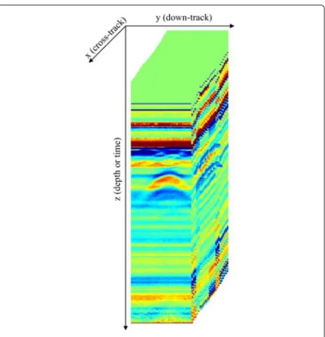
system [33] (see Fig. 4). This system collects 51 chan-nels of data. Adjacent chanchan-nels are spaced approximately five centimeters apart in the cross-track direction, and sequences (or scans) are taken at approximately 1-cm down-track intervals. Each A-scan, that is, the measured waveform that is collected in one channel at one down-track position, contains 416 time samples at which the GPR signal return is recorded. We often refer to the time index as depth although, since the radar wave is travel-ing through different media, this index does not represent a uniform sampling of depth. Thus, we model an entire collection of input data as a three-dimensional matrix of sample values,S(z,x,y),z=1,· · ·, 416;x=1,· · ·, 51;y= 1,· · ·,NS, whereNSis the total number of collected scans, and the indices z, x, and y represent depth, cross-track position, and down-track positions respectively. A collec-tion of scans, forming a volume of data, is illustrated in Fig. 5.
Figure 6 displays several B-scans (sequences of A-scans) both down-track (formed from a time sequence of A-scans from a single sensor channel) and cross-track (formed from each channel’s response in a single sample). The surveyed object position is highlighted in each figure. The objects scanned are (a) a high-metal content antitank mine, (b) a low-metal antipersonnel mine, and (c) a wood block.
Raw GPR data needs to be preprocessed and pre-screened. Preprocessing includes ground-level alignment and signal and noise background removal. Prescreening is needed to focus attention and identify regions with subsurface anomalies. For this step, we use the adaptive least mean squares (LMS) prescreener [34]. The LMS flags locations of interest utilizing a computationally inexpen-sive algorithm so that more advanced algorithms can be applied only on the small subsets of data flagged by the prescreener.
In our experiments, data sets are comprised of a variety of mine and background signatures. In particular, we use
Fig. 4NIITEK vehicle mounted GPR system
Fig. 5A collection of few GPR scans
data collected from outdoor test lanes at three different locations. The first two locations, site 1 and site 2, were temperate regions with significant rainfall, whereas the third collection, site 3, was a desert region. The lanes are simulated roads with known mine locations. Multiple data collections were performed at each site at different dates. The statistics of these data sets are reported in Table 1. Data cubes of size (15 scans, 7 channels, 416 depths) were extracted from each scan position flagged by the pre-screener and are presented to the classifier to discriminate between mines and false alarms.
5.2 Feature extraction
The goal of the feature extraction step is to transform original GPR data into a sequence of observation vectors. We use two types of features that have been proposed and used independently. Each feature represents a differ-ent interpretation of the raw data and aims at providing a good discrimination between mine and clutter signatures. These features are outlined in the following subsections.
5.2.1 EHD features
This feature is based on the edge histogram descriptor [9] (EHD) and characterizes edges in the spatial domain.
Table 1Data collections
Total number of Mine encounters False alarms prescreened alarms
D1 2477 732 1745
D2 1343 724 619
Fig. 6NIITEK radar down-track and cross-track (at position indicated by a line in the down-track) B-scans pairs foraan Anti-Tank (AT) mine,ban Anti-Personnel (AP) mine, andca non-metal clutter alarm
The EHD captures the salient properties of the 3D alarms in a compact and translation invariant representation. It extracts edge histograms capturing the frequency of occurrence of edge orientations in the data associated with a ground position. Simple edge detector operators are used to identify edges and group them into five cat-egories: vertical, horizontal, diagonal, anti-diagonal, and isotropic (non-edge). Each B-scan position is then rep-resented by a five-dimensional observation vector. Each dimension of this vector represents the percentage of pixels (in a small interval along the depth) that belong to each of the five edge categories.
5.2.2 Gabor features
Gabor features characterize edges in the frequency domain at multiple scales and orientations and are based on Gabor wavelets [7]. This feature is extracted by expand-ing the signature’s B-scan (depth vs. down-track) usexpand-ing a bank of scale and orientation selective Gabor filters. Expanding a signal using Gabor filters provides a local-ized frequency description. In our experiments, we use a bank of filters tuned to the combination of three scales and four orientations. Each observation is then represented by a 12-dimension feature vector.
5.3 Ensemble HMM implementation and results
In all experiments reported in this paper, we use a sixfold cross validation for each data collectionDl,l ∈ {1, 2, 3}.
For each fold, a subset of the data (DlTrn) is used for training and the remaining data (DlTst) is used for testing.
OlFeatTrn denotes the set of observation sequences extracted
from datasetDl, using one of the feature extraction
meth-ods, “Feat” (EHD or Gabor).
The first step of the eHMM is the similarity matrix com-putation. This step requires fitting an individual HMM model for each sequence in the training data OlFeatTrn.
Figure 7 shows the log-likelihood and path mismatch penalty matrices for a training collection that has 521 mines and 1471 clutter signatures (first training fold of D1 using EHD features, O1EHDTrn1). In these figures, the
Fig. 7Log-likelihood and path mismatch penalty matrices for a large collection of mine and clutter signatures.aLog-likelihood true andbpath mismatch penalty
as alarms from the same class are expected to be more similar to each other than alarms from different classes. However, they could be used to validate our similarity (and penalty) measures in the log-likelihood space. A more important observation is that within each diagonal block, sub-blocks can be extracted. This is an indication of the existence of different clusters within the mines (and the clutter) themselves.
In the second step, the similarity matrix is transformed into a distance matrix, D, using (10). The hierarchi-cal clustering algorithm [18] is then applied, using D with a fixed number of clusters K = 10, to identify sub-categories within the training data. For both the discrete and continuous versions, using any of the fea-tures and datasets, the eHMM clustering step success-fully assigns groups of similar alarms into clusters. For instance, in Fig. 9, we show the hierarchical clustering results of the first crossvalidation fold of the eCHMM using the EHD features on datasetD1. As it can be seen
in Fig. 9a, we have a group of clutter dominated clus-ters (in brown) and a second group of clusclus-ters dominated by mines (in blue). In Fig. 8, we show sample signatures that belong to clusters 1, 6, and 10. As it can be seen from Figs. 8 and 9a, cluster 1 has only clutter and clus-ters 6 and 10 are composed exclusively of mine alarms. The mines that belong to cluster 6 have typically strong mine signatures. These mines, as shown in Fig. 9b, c, are typically mines with high metal content that are buried at shallow depths. The mines that belong to cluster 10 have weak GPR signatures. These mines, as shown in Fig. 9b, c, are typically mines with weak signatures that are either low metal mines or mines buried at deep depths.
Additional details of the clusters’ contents per mine type and per burial depth are shown in Fig. 9b, c. To summa-rize, the training data includes four homogeneous clusters (Clusters 6, 7, and 10 contain only mines and cluster 1 has only clutter). The remaining clusters (2, 3, 4, 5, 8, and 9)
Fig. 9eCHMM hierarchical clustering results ofO1EHDTrn1: distribution of the alarms in each cluster:aper class,bper type,cper depth
are mixed. Therefore, using the notation of Algorithm 1, we define our eHMM as:
⎧ ⎪ ⎪ ⎨ ⎪ ⎪ ⎩
λBW
i =
λ(F)
1 ,λ(6M),λ7(M),λ(10M)
, λMCE
j =
λ(M) j ,λ
(C) j
,j∈ {2, 3, 4, 5, 8, 9}, λVB
k = ∅.
(16)
In Table 2, we report the means and the weights of the components of each state of the BW-trained eCHMM model for cluster 6,λ(6M), as well as its transition proba-bility matrix. Cluster 6 contains “typical” mines that have
Table 2λM6 CHMM model parameters of cluster 6
Means Weights
H V D A N w
s1 c11 0.21 0.17 0.41 0.07 0.13 g11 0.30
c12 0.36 0.12 0.25 0.11 0.17 g12 0.22
c13 0.15 0.18 0.23 0.06 0.37 g13 0.49
s2 c21 0.42 0.09 0.25 0.12 0.13 g21 0.30
c22 0.37 0.10 0.10 0.30 0.13 g22 0.20
c23 0.59 0.05 0.10 0.12 0.14 g23 0.50
s3 c31 0.38 0.11 0.10 0.26 0.16 g31 0.21
c32 0.20 0.17 0.07 0.43 0.13 g32 0.30
c33 0.14 0.20 0.06 0.25 0.36 g33 0.49
A
s1 s2 s3
s1 0.73 0.27 0.00
s2 0.00 0.67 0.33
s3 0.00 0.00 1.00
strong-edge and near-perfect hyperbolic shape signatures with succession of statess1,s2, ands3. Recall thats1,s2, ands3correspond respectively to the rising (Dg), flat (Hz), and falling (Ad) edges within the mine signature. There-fore, all the components ofs1(resp.s3) have their diagonal edge higher (resp. lower) than the anti-diagonal one. Sim-ilarly, components ofs2have higher horizontal edge and comparable diagonal and anti-diagonal edges. As it can be seen in the transition matrix of Table 2, the probability of staying ins1(resp.s2) is approximately three times (resp. two times) the probability of moving tos2(resp.s3).
Table 3λM10CHMM model parameters of cluster 10
Means Weights
H V D A N w
s1 c11 0.14 0.13 0.17 0.08 0.48 g11 0.27
c12 0.26 0.11 0.20 0.06 0.37 g12 0.40
c13 0.16 0.04 0.10 0.05 0.66 g13 0.32
s2 c21 0.30 0.07 0.10 0.14 0.39 g21 0.50
c22 0.48 0.05 0.11 0.14 0.22 g22 0.28
c23 0.27 0.12 0.07 0.37 0.16 g23 0.21
s3 c31 0.09 0.11 0.03 0.18 0.59 g31 0.60
c32 0.22 0.17 0.05 0.36 0.20 g32 0.04
c33 0.10 0.20 0.02 0.31 0.36 g33 0.36
A
s1 s2 s3
s1 0.74 0.26 0.00
s2 0.00 0.89 0.11
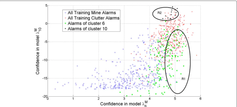
Fig. 10Scatter plot of the confidences of the training data in cluster modelλ(6M)(strong mines) vs. cluster modelλ(10M)(weak mines)
Table 3 shows the BW-trained eCHMM model for clus-ter 10, λ(10M). Recall that cluster 10 contains only mine signatures that have a low metal content and/or are buried at 4" or deeper, as it can be seen in Fig. 9c. Therefore, the alarms in cluster 10 are expected to have weak sig-natures and weak edge features. This could explain the large non-edge component of most of the states’ means components of λ(10M) reported in Table 3, compared to the non-edge components ofλ(6M)’s states representatives. Nevertheless, the states representatives still characterize the hyperbolic shape of a typical mine signature, i.e., the succession ofDg−Hz−Ad states. For instance, all s1 components means have their diagonal Ddimension larger than the anti-diagonalAdimension. For the tran-sition matrix, we notice that λ(10M) is more stationary in s2, with a probability of 0.89, compared to λ(6M). This means that, on average, sequences belonging to cluster 10 have a large number of observations with flat edge and
fewer observations with strong diagonal or anti-diagonal edges.
Figure 10 shows the scatter plot of the confidences assigned by λ(6M) and λ(10M) to all the training data. In this figure, we display clutter and mine signatures that belong to each cluster using different symbols and colors. Even though the two models are dominated by mine sig-natures, we see that not all confidence values are highly correlated. On one hand, some strong mine signatures, particularly those belonging to cluster 6, have high log-likelihoods in model λ(6M) and lower log-likelihoods in modelλ(10M)(lower right side of the scatter plot, region R1). This can be attributed to the fact that cluster 6 contains mainly strong mines and is more likely to yield high log-likelihood when testing a strong mine signature. On the other hand, in region R2, the performance ofλ(10M)is better as it gives higher likelihood values to the “weak” mines in that region, particularly those belonging to cluster 10.
Fig. 12ROCs generated by the eCHMM (solid lines) and baseline CHMM (dashed lines) classifiers usingD1andaEHD,bGabor features
In fact, this result is expected because cluster 10 contains weak mine signatures.
The main conclusion that we can draw from the above example is thatλ(6M)andλ(10M)are very different and char-acterize two distinct subsets of the training data. The standard HMM approach would combine all alarms to learn a single model for mines (weak and strong) and a single model for clutter.
In the final step, the eHMM mixture is combined using a single-layer ANN. The ANN parameters are trained to fit the responses of the eHMM mixture models to the training data labels.
5.4 eHMM vs. baseline HMM results
In this section, we compare the performance of the pro-posed eHMM to the baseline HMM [5]. For the eHMM, we show the results using the ANN fusion and the hierarchical agglomerative clustering with K = 20. In Fig. 11a, b, we show the ROCs generated by the dis-crete versions of the eHMM and the baseline HMM on datasetD1, using EHD and Gabor features. Similarly, in
Fig. 12a, b, we report the ROCs generated by the contin-uous versions, i.e., the eCHMM and the baseline CHMM, on datasetD1. As it can be seen, in all the ROCs of Figs. 11
and 12, at a given false alarm rate (FAR), the eHMM has a better probability of detecting targets. For instance, in Fig. 11a, at a FAR of 10 %, the eDHMM using EHD features successfully identifies 94 % of the mines while the baseline DHMM identifies only 87 % of the targets. At the same FAR of 10 %, the ROCs of Fig. 12a show that the eCHMM successfully identifies 95 % of the tar-gets while the baseline CHMM probability of detection is 85 %.
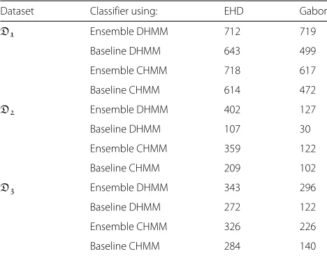
The results for all three datasets are summarized in terms of the Area Under ROC Curve (AUC) and are reported in Table 4. As it can be seen, in all experiments, the eHMM outperforms the baseline HMM.
6 Conclusions
In this work, we have proposed a novel ensemble HMM classification method that is based on clustering sequences in the log-likelihood space. The eHMM uses multiple HMM models and fuses them for final deci-sion making. We hypothesized that the data are generated by multiple models. These different models reflect the fact that samples from the same class can have different characteristics resulting in large intra-class variability.
The eHMM, in its discrete and continuous versions, was implemented and evaluated using large collections of landmine GPR data. We examined the intermediate steps of the eHMM and compared its performance to the base-line HMM. Results on three GPR data collections show that the proposed method can identify meaningful and coherent HMM mixture models that describe different properties of the data. Each individual HMM character-izes a group of data that share common attributes. The experiments show that the proposed eHMM intermediate results are inline with the expected behavior. The results
Table 4AUC of the ensemble HMM and baseline HMM classifiers
Dataset Classifier using: EHD Gabor
D1 Ensemble DHMM 712 719
Baseline DHMM 643 499
Ensemble CHMM 718 617
Baseline CHMM 614 472
D2 Ensemble DHMM 402 127
Baseline DHMM 107 30
Ensemble CHMM 359 122
Baseline CHMM 209 102
D3 Ensemble DHMM 343 296
Baseline DHMM 272 122
Ensemble CHMM 326 226
also indicate that, for both the continuous and discrete versions, the proposed method outperforms the baseline HMM that uses one model for each class in the data.
Endnote
1The details of the landmine detection application
using GPR signatures will be presented in section 5.
Competing interests
The authors declare that they have no competing interests.
Acknowledgements
This work was supported in part by U.S. Army Research Office Grants Number W911NF-13-1-0066 and W911NF-14- 1-0589. The views and conclusions contained in this document are those of the authors and should not be interpreted as representing the official policies, either expressed or implied, of the Army Research Office, or the U.S. Government.
Received: 8 April 2015 Accepted: 4 August 2015
References
1. Landmine Monitor Report, (2013). http://www.themonitor.org/ 2. TR Witten, inSPIE Conf Detection and Remediation Technologies for Mines
and Minelike Targets III. Present state of the art in ground-penetrating radars for mine detection (Orlando, FL, 1998), pp. 576–586
3. PD Gader, H Frigui, BN Nelson, G Vaillette, JM Keller, inSPIE Conf Detection and Remediation Technologies for Mines and Minelike Targets IV. New results in fuzzy set based detection of landmines with GPR (Orlando, FL, 1999), pp. 1075–1084
4. PD Gader, B Nelson, H Frigui, G Vaillette, JM Keller, Fuzzy logic detection of landmines with ground penetrating radar. Signal Process. Special Issue Fuzzy Logic Signal Process.80, 1069–1084 (2000)
5. PD Gader, M Mystkowski, Y Zhao, Landmine detection with ground penetrating radar using hidden Markov models. IEEE Trans. Geosci. Remote Sensing.39, 1231–1244 (2001)
6. H Frigui, DKC Ho, PD Gader, Real-time landmine detection with ground-penetrating radar using discriminative and adaptive hidden Markov models. EURASIP J. Appl. Signal Process.12, 1867–1885 (2005) 7. H Frigui, O Missaoui, PD Gader, inSPIE Conf. Detection and Remediation Technologies for Mines and Minelike Targets XII. Landmine detection using discrete hidden Markov models with Gabor features (Louisville, KY, USA, 2007)
8. H Frigui, PD Gader, S Kotturu, inSPIE Conf. Detection and Remediation Technologies for Mines and Minelike Targets. Detection and discrimination of landmines in ground penetrating radar using an eigenmine and fuzzy membership function approach, (2004). doi:10.1109/TFUZZ.2008.2005249 9. H Frigui, PD Gader, inProceedings of the IEEE International Conference on
Fuzzy Systems. Detection and discrimination of land mines based on edge histogram descriptors and fuzzy k-nearest neighbors (Vancouver, BC, Canada, 2006)
10. A Karem, A Fadeev, H Frigui, Gader, P, inSociety of Photo-Optical Instrumentation Engineers (SPIE) Conference Series. Comparison of different classification algorithms for landmine detection using GPR, vol. 7664, (2010), p. 2. doi:10.1117/12.852257
11. PA Torrione, KD Morton, R Sakaguchi, LM Collins, Histograms of oriented gradients for landmine detection in ground-penetrating radar data. Geosci. Remote Sens. IEEE Trans.52(3), 1539–1550 (2014). doi:10.1109/ TGRS.2013.2252016
12. O Missaoui, H Frigui, P Gader, inGeoscience and Remote Sensing Symposium (IGARSS), 2010 IEEE International. Model level fusion of edge histogram descriptors and Gabor wavelets for landmine detection with ground penetrating radar, (2010), pp. 3378–3381. doi:10.1109/IGARSS. 2010.5650350
13. O Missaoui, H Frigui, P Gader, inMachine Learning and Applications, 2009. ICMLA ’09. International Conference On. Discriminative multi-stream discrete hidden Markov models, (2009), pp. 178–183. doi:10.1109/ICMLA. 2009.121
14. O Missaoui, H Frigui, P Gader, Multi-stream continuous hidden Markov models with application to landmine detection. EURASIP J. Adv. Signal Process.1(2013). doi:10.1186/1687-6180-2013-40
15. CR Ratto, KD Morton, LM Collins, PA Torrione, inGeoscience and Remote Sensing Symposium (IGARSS), 2011 IEEE International. A hidden Markov context model for GPR-based landmine detection incorporating stick-breaking priors, (2011), pp. 874–877. doi:10.1109/IGARSS.2011. 6049270
16. LR Rabiner, inProceedings of the IEEE. A tutorial on hidden Markov models and selected applications in speech recognition (San Francisco, CA, USA, 1989), pp. 257–286
17. S Theodoridis, K Koutroumbas,Pattern Recognition, Fourth Edition. (Academic Press, Inc, Orlando, FL, USA, 2009)
18. R Duda, P Hart,Pattern Classification and Scene Analysis. (John Wiley and Sons, New York, 1973)
19. LE Baum, T Petrie, Statistical Inference for Probability Functions of Finite State Markov Chains. Ann. Math. Stat.37, 1554–1563 (1966)
20. J Paisley, L Carin, Hidden Markov models with stick-breaking priors. Signal Process. IEEE Trans.57(10), 3905–3917 (2009). doi:10.1109/TSP.2009. 2024987
21. LE Baum, T Petrie, Statistical inference for probabilistic functions of finite state Markov chains. Ann. Math. Stat.37(6), 1554–1563 (1966). doi:10.2307/2238772
22. JH Ward, Hierarchical grouping to optimize an objective function. J. Am. Stat. Assoc.58(301), 236–244 (1963)
23. JH Holland,Adaptation in Natural and Artificial Systems. (MIT Press, Cambridge, MA, USA, 1992)
24. S Kirkpatrick, CD Gelatt, MP Vecchi, Optimization by Simulated Annealing. Science.220(4598), 671–680 (1983). doi:10.1126/science.220.4598.671. http://www.sciencemag.org/cgi/reprint/220/4598/671.pdf
25. B-H Juang, W Chou, C-H Lee, Minimum Classification Error Rate Methods for Speech Recognition. Trans. Speech Audio Process.5(3), 257–265 (1997) 26. DJC MacKay,Information Theory, Inference and Learning Algorithms.
(Cambrdige University Press, New York, 2003)
27. AK Jain, RC Dubes,Algorithms for Clustering Data. (Prentice Hall, Upper Saddle River, NJ, USA, 1988)
28. JC Bezdek,Pattern Recognition with Fuzzy Objective Function Algorithms. (Kluwer Academic Publishers, Norwell, MA, USA, 1981)
29. G Fumera, F Roli, A theoretical and experimental analysis of linear combiners for multiple classifier systems. IEEE Trans. Pattern Anal. Mach. Intell.27(6), 942–956 (2005). doi:10.1109/TPAMI.2005.109
30. DS Lee, SN Srihari, inICDAR ’95: Proceedings of the Third International Conference on Document Analysis and Recognition (Volume 1). A theory of classifier combination: the neural network approach (IEEE Computer Society Washington, DC, USA, 1995), p. 42
31. MI Jordan, RA Jacobs, inNIPS. Hierarchies of adaptive experts (Denver, 1991), pp. 985–992
32. DE Rumelhart, GE Hinton, RJ Williams, Learning internal representations by error propagation, 318–362 (1986). ISBN:0-262-68053-X
33. KJ Hintz, inProceedings of the SPIE Conference on Detection and Remediation Technologies for Mines and Minelike Targets IX. SNR
improvements in Niitek ground penetrating radar (Orlando, FL, USA, 2004) 34. PA Torrione, CS Throckmorton, LM Collins, Performance of an adaptive