Closed-loop integration of planning, scheduling and multi-parametric nonlinear control

(1)

Contents lists available at ScienceDirect

Computers

and

Chemical

Engineering

journal homepage: www.elsevier.com/locate/compchemeng

Closed-loop

integration

of

planning,

scheduling

and

multi-parametric

nonlinear

control

Vassilis

M.

Charitopoulos,

Lazaros

G.

Papageorgiou

,

Vivek

Dua

∗

DepartmentofChemicalEngineering,CentreforProcessSystemsEngineering,UniversityCollegeLondon,TorringtonPlace,LondonWC1E7JE,United Kingdom

a

r

t

i

c

l

e

i

n

f

o

Articlehistory: Received10January2018 Revised15June2018 Accepted26June2018 Availableonlinexxx Keywords: Multi-parametricprogramming Enterprisewideoptimization Integration

Processplanning Rescheduling

Closed-loopoptimization

a

b

s

t

r

a

c

t

Inthisarticle,motivatedbytheneedforeﬃcientclosed-loopimplementationofthecontrolobjectivesset withintheintegratedplanning,schedulingandcontrol(iPSC)problemweintroduceanovelframework thatenablesitsonlinesolutionunderdynamicdisturbances.Weintroducetheconceptofmulti-setpoint explicitcontrollers throughthe useof anewmulti-parametricnonlinear programmingalgorithmand develop arigorousrescheduling mechanism thatmitigates the impact ofthe dynamicdisruptions on theoperationaldecisionsofplanningandscheduling.Theoverallclosed-loopproblemisformulatedas mixedintegerlinearprogramwiththecontrolproblemintegratedviaanouterloop.Thebeneﬁtsofthe proposedframeworkarehighlightedthroughtwocasestudiesand theresultsindicatethenecessityof consideringdynamicdisruptionswithinthescopeoftheintegratedproblem.

1. Introduction

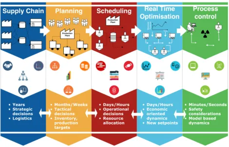
Volatile global market environment, increasing competition and the need for reduction in cost and environmental impact are only a few of the reasons that have led the process industries to seek more responsive and integrated operations. Enterprise Wide Optimisation (EWO) aims to address the aforementioned chal- lenges and provide the industries with tools that can serve as means for enhanced proﬁtability and more sustainable operations ( Grossmann, 2012 ). Within the EWO scope one seeks for more integrated decision making via the coordinated optimisation of the supply chain functionalities so as to holistically guarantee the ef- ﬁcient information sharing and optimal operations among the different levels of decision making. A conceptual representation of the EWO scope is given in Fig. 1 , where the different levels of decision making, the key decisions and timescales involved are summarised. Some of the most important operational functionalities of the process industries comprise of production planning, scheduling, real time optimisation and control. To this end, the process systems engineering (PSE) community has focused on the development of methods for their integration so as to exploit the inherent synergies and prevent suboptimal operations due to negligence of their underlying interdependence

∗ _{Corresponding}_author.

E-mailaddress:[email protected](V.Dua).

( Chu and You, 2015; Grossmann, 2012; Harjunkoski et al., 2014 ). While traditionally, the problems of planning, scheduling and control have been modelled and solved in a decoupled and sequential fashion due to more favorable computational requirements. Re- cently a number of research works have been devoted to their integration ( Charitopoulos et al., 2017b; Gutierrez-Limon et al., 2014; Shi et al., 2015 ). Integration of planning and scheduling has been studied extensively in the past and their simultaneous optimisation has proven to result in improved proﬁtability since decisions such as inventory calculation and production targets from the planning problem are highly interconnected with the optimal resource al- location which stems from the scheduling problem ( Castro et al., 20 04; Maravelias and Sung, 20 09 ). Another signiﬁcant trend is to- wards the integration of scheduling and control and a considerable amount of research work has been reported on that problem ( Chu and You, 2015 ). While scheduling deals with the optimal allo- cation of limited resources and the sequencing of tasks, the underlying dynamics of the systems which are mostly dealt by the control functionality can highly affect the duration of changeovers and the quality of products manufactured during the production periods. It follows naturally that the integration of planning, scheduling and control (iPSC) can result in more optimal operations since the underlying synergies among the individual problems can enhance process operations. Unfortunately, if enhanced operations is the gift of integration, its price is quite high as it results in large- scale, typically non-convex, optimisation problems and extensive computational times that prohibit its application to large scale https://doi.org/10.1016/j.compchemeng.2018.06.021

(2)

Fig.1. Enterprisewideoptimisationscope.

Indexofabbreviations.

Abbreviation Meaning

CAD CylindricalAlgebraicDecomposition CR CriticalRegion

EWO EnterpriseWideOptimisation

iPSC integratedPlanningSchedulingandControl iSC integratedSchedulingandControl KKT Karush–Kuhn–Tucker

MILP MixedIntegerLinearProgramming MINLP MixedIntegerNonlinearProgramming MMA methyl-methacrylate

MPC ModelPredictiveControl mp-P Multi-parametricProgramming

mp-MPC Multi-setpointexplicitModelPredictiveControl NLP NonlinearProgramming

NLMPC NonlinearModelPredictiveControl OFC ObjectiveFunction’sCoeﬃcient PSE ProcessSystemsEngineering RHS right-handside

RTO RealTimeOptimisation SISO SingleInputSingleOutput TSP TravellingSalesmanProblem

systems. To this end, decomposition and simpliﬁcations of the integrated problem have been proposed in the literature so as to allow for the study of large-scale systems ( Pistikopoulos and Diangelakis, 2016; Zhuge and Ierapetritou, 2016 ).

The efficient online computation of the decisions involved in the iPSC under uncertain conditions remains an open challenge ( Dias and Ierapetritou, 2016 ). The main goal of the present work is to propose a framework for the closed-loop iPSC under dynamic disturbances and illustrate how the consideration of uncertain operating conditions accentuates the need for integration among the different levels of decision making. In this article, we build on the developments previously presented by our group ( Charitopoulos et al., 2017b ) for the open-loop case and with the use of multi-parametric programming a novel framework for the closed-loop implementation of the iPSC is proposed. The key elements of the proposed framework involve: (i) linear metamodels that correlate transition times and costs based on closed-loop simulations of the underlying dynamic systems, (ii) the implementation of novel multi-parametric nonlinear model predictive controllers and (iii) an optimisation based algorithm for the efficient rescheduling that mitigates the impact of disturbances on the online implementation of the integrated problem. The remainder of the article is structured as follows: first a literature review is presented on the topic of integrating control with operations and the

need for a closed-loop framework for iPSC is underlined. Next, the key elements of the proposed framework are introduced; we brieﬂy summarise the model employed for the open-loop iPSC and then the role of multi-parametric programming in the closed-loop implementation of the iPSC is presented. Subsequently, the overall closed-loop framework is presented in detail with its necessity and eﬃciency been shown through two case studies. Finally, conclud- ing remarks and future research directions are discussed.

2. Literaturereview

Integrating control and operations has attracted signiﬁcant amount of attention from the research community because of the potential beneﬁts that result from the exploitation of their underlying synergies ( Chu and You, 2015; Dias and Ierapetritou, 2016 ). Control relevant decisions provide an important set of data, such as transition times and production rates, which are crucial for modelling and solving in an optimal manner the scheduling problem. On the other hand, sequencing decisions are needed by the control decision layer so as to proceed with the manipulation of the dynamics of the production system.

The aforementioned interactions between cyclic scheduling and control were examined by Flores-Tlacuahuac and Gross- mann (2006) and the authors showed how their open-loop integration can yield better results when compared to the conventional sequential solution of the problems. The closed-loop integration of cyclic scheduling and control (iSC) for continuous processes was studied by Zhuge and Ierapetritou (2012) and a model predictive control inspired mechanism was proposed so as to mitigate the effect that disturbances had on the execution of the schedule. Through a number of case studies the authors demonstrated how the closed-loop iSC can cope with disturbance rejection during production and transition periods. An alternative methodology for the closed-loop iSC has been reported in Chu and You (2012) . The authors, in an oﬄine step, generated a number of PI-controllers for each possible transition and studied the integrated problem as the optimal simultaneous scheduling and controller selection. In order to achieve fast computational times, the resulting MINLP with frac- tional objective function was solved using Dinkelbach’s algorithm. Aiming to reduce the time needed for the solution Zhuge and Ierapetritou (2014) suggested the use of multi-parametric model predictive control within the context of iSC. First, the original nonlinear dynamics of the underlying production system were lin- earised and then the explicit controller was designed through the

(3)

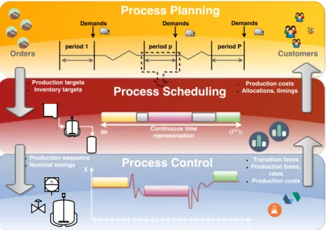
Fig.2. Conceptualrepresentationoftheintegratedplanning,schedulingandcontrolproblemalongwiththerelatedinterdependentdecision.

solution of the corresponding multi-parametric program. The explicit solutions were then incorporated in the scheduling model as a set of big-M constraints and the overall iSC was modelled as an MILP. Later on, the same authors proposed the use of fast MPC ( Zhuge and Ierapetritou, 2015 ) and in that work piecewise aﬃne approximations of the nonlinear dynamics were employed.

One of the main bottlenecks in the integrated problem is the time-scale separation among the different layers of decision making. To this end, Baldea et al. (2015) proposed the use of lower- dimensional dynamic models and embedded them in the scheduling formulation as a set of soft constraints. In their time scale- bridging approach, a scheduling oriented MPC was also employed so as to synchronise the calculations between MPC and scheduling. However, when the demand is not assumed to follow a periodic pattern, the integration of planning along with scheduling and control becomes necessary. The iPSC is an inherently multi-scale problem for which one aims to optimise simultane- ously the decisions involved in the levels of planning, scheduling and control so as to improve process operations and take explic- itly into account their interdependence. As shown in Fig. 2 , the different problems communicate via a number of interconnected decisions and there is information flow throughout. Gutierrez- Limon et al. (2014) extended the work of Flores-Tlacuahuac and Grossmann (2006) and formulated the problem as a large-scale monolithic MINLP along with a nonlinear model predictive control (NLMPC); a number of case studies were presented that resulted in large computational times for the solution of the integrated problem while disturbance rejection was not considered. Recently, in Gutierrez-Limon et al. (2016) a preliminary study on the effect of rush orders on the optimal solution of the iPSC was conducted and a number of heuristics were proposed in a reactive strategy sense. Shi et al. (2015) motivated by the need for faster computational times, proposed a decomposition framework based on flexible recipes involving all the potential transition between products. The overall flexible recipe iPSC was modelled as an MILP and the bilevel decomposition method by Dogan and Grossmann (2006) was employed to further enhance the computational behavior of the proposed framework. In our previous work ( Charitopoulos et al., 2017b ) we studied the iPSC of continuous processes using a traveling salesman problem (TSP) based model that proved to allow for significant computational savings when

compared to the time slot based formulations. We proposed the use of linear metamodels that correlate transition time and cost and under deterministic assumptions solved the integrated problem as an MILP whose optimal solution was equivalent to the one computed by the monolithic nonconvex MINLP.

Even though the problem of integrating control with operations has received considerable attention from the research community, no previous work has considered the iPSC under dynamic disturbances, i.e. closed-loop iPSC. For the online implementation of the iPSC to be effective and realistic one would have to account for dynamic disruptions at the level of control and develop an uncertainty-aware framework so as to secure optimal operations and real time execution. Due to the integrated nature of the problem it is reasonable to expect an immediate effect on the scheduling and planning decisions whenever the dynamics of the system are signiﬁcantly disturbed.

The need for eﬃcient reactive policies in the context of process scheduling has been long underlined in the open literature ( Aytug et al., 2005 ). A least impact heuristic proposed by Kanakamedala et al. (1994) was among the ﬁrst works pub- lished that considered the problem of reactive scheduling in multi- product batch plants. The reactive scheduling of batch processes was also studied by Vin and Ierapetritou (20 0 0) and the authors considered two different kinds of disturbances, rush orders and machine breakdowns. In their work, the rescheduling mechanism is developed by the means of a repetitive solution of a reduced MILP problem every time new information about disruptions becomes available to the plant. The degree of deviation from the original schedule is also controlled through the use of a penalty in the objective function. Scheduling disruptions and reactive policies were studied by Mendez and Jaime (2004) , where the authors used continuous time representation for multistage batch facilities and formulated the rescheduling problem as an MILP. The impact of rescheduling penalties in the objective function on the quality of the reschedule solution was also studied by Kopanos et al. (2008) . Novas and Henning (2010) proposed a reactive scheduling framework based on a combination of constraint programming and explicit object oriented domain model that resulted in nearly optimal solutions at relatively low computational times. The use of multi- parametric programming has also been reported in the literature as a way of developing a reactive policy in scheduling problems by

(4)

several researchers ( Kopanos and Pistikopoulos, 2014; Li and Ier- apetritou, 2008 ). Recently, Maravelias and co workers ( Gupta et al., 2016; Subramanian et al., 2012 ) in a series of papers based on the state-space interpretation of the scheduling of batch processes studied the effect of different factors on the derivation of periodic and reactive schedules.

In the following section, we review the mathematical developments proposed in the present work as a means for the real-time closed-loop implementation of the iPSC decisions along with an MIP-based rescheduling mechanism.

3. Mathematicalformulations

In this section the main methodological components of the proposed framework are presented. First, we brieﬂy review on the open-loop problem and its related modelling aspects. Next, the concept of multi-setpoint explicit controllers is presented and lastly the overall framework along with the corresponding algorithmic steps are outlined.

3.1.Modellingtheintegratedplanning,schedulingandcontrol problem

3.1.1. Open-loopintegrationofplanning,schedulingandcontrol The open-loop case of iPSC was treated in a work recently presented by our group where a TSP based model was proposed for the integrated problem along with the use of linear metamodels ( Charitopoulos et al., 2017b ). Compared to the time slot based formulations used in the literature ( Gutierrez-Limon et al., 2014; Shi et al., 2015 ), in the TSP based formulation there is not a ﬁxed number of time slots to be postulated a priori but rather implicit unique pairs of products/tasks that need to be sequenced. For sequencing purposes, the time slot based formulations require the introduction of binary variables to assign products to time slots for each planning period that tend to increase the solution times for large planning horizons. On the contrary, the TSP based formulations track the sequencing of products/tasks in a similar way to the classic TSP problem using binary variables to model the relevant changeovers and computational saving compared to the time slot based formulation are achieved ( Aguirre et al., 2017; Charitopoulos et al., 2017a; 2017b; Liu et al., 2008 ).

We brieﬂy review the main equations for ease of understanding while the interested reader is referred to our earlier works for detailed exposition on the computational behavior and analysis of the proposed model ( Charitopoulos et al., 2017b; Liu et al., 2008 ). In the TSP-based model, a hybrid time formulation is employed with planning periods modelled as discrete time points whereas within each point, continuous time formulation of

θ

pupduration is consid-

ered. Within each period only one product (i) can be ﬁrst (F _ip) and last (L _ip) as shown by Eqs. (1) and (2) while the assignment of the products in each period is done via Eqs. (3) and (4) with the use of binary variable E ip. N i Fip=1,

∀

p (1) N i Lip=1,

∀

p (2) Fip≤Eip,

∀

i, p (3) Lip≤Eip,

∀

i, p (4)

Sequencing of different products (i, j) within the same planning period is tracked with the binary variable Z ijp and Eqs.

(5) and (6) while between adjacent planning periods changeovers are tracked with the binary variable ZF ijp and Eqs. (7) and (8) .

N i=j Zijp=Ejp−Fjp,

∀

j,p (5) N j=i Zijp=Eip−Lip,

∀

i,p (6) N i ZFijp=Fjp,

∀

j, p > 1 (7) N j ZFijp=L_i,p₋₁,

∀

i, p > 1 (8)

In order to avoid infeasible production subcycles and the enu- meration of symmetric solutions, the integer variable O _ip along with Eqs. (9) –(11) are used.

Ojp−

(

Oip+1

)

≥ −M

(

1−Zijp

)

,

∀

i, j∈I, j=i, p (9) Oip≤M·Eip,

∀

i, p (10) Fip≤Oip≤ N i Eip,

∀

i,p (11)

where M is a big number which for the sake of tight relaxation is equated to the cardinality of the set of products. Within each planning period, the processing (T _ip) and transition time

(

T trans

ijp , TF trans ijp

)

are modelled as continuous variables. More speciﬁcally, production times are bounded between minimum and maximum times,

θ

lo

p

and

θ

_puprespective as shown by Eq. (12) . Moreover, the changeover time between adjacent periods are allowed to split into two parts (CT1 p and CT2 p) as shown by Eq. (13) while the overall time bal-

ance for each period is given by Eq. (14) . The variables CT1 p and

CT2 p are employed to allow for instances where a transition time

can be modelled to be split between two adjacent periods and thus result in more eﬃcient utilisation of resources ( Kopanos et al., 2010 ).

θ

lo pEip≤Tip≤

θ

pupEip,

∀

i, p (12) CT1p+CT2p−1= i j TFtransijp ,

∀

p> 1 (13) N i T ip+ N i N j=i Ttrans ijp +CT1p_|p>1+CT2p|p<|P|=

θ

up p ,

∀

p (14)

Notice that Eq. (14) accounts for idle production time by con- sidering a relevant dummy product. The amount of product i produced during period p (Pr ip) is calculated based on Eq. (15) , by

assuming constant production rate (r _i). Given product demand per customer (D cip), backlog (B cip), sales (S cip) and inventory (V ip) cal-

culations are based on Eqs. (16) and (17) respectively. Also minimum ( V min

ip ) and maximum ( V maxip ) inventory levels can be speciﬁed

by Eq. (18) .

Prip=riTip,

∀

i, p (15)

(5)

Vip=Vi,p−1+Prip−

c

Scip,

∀

i, p (17)

Vmin_i ≤V ip≤V imax,

∀

i, p (18) Transitions times are allowed to be decision variables but in order to avoid the resulting bilinear terms, Glover linearisation is employed as shown in Eqs. (19) –(26) . For the purpose of the linearisation two more artiﬁcial positive variables are deﬁned,

τ

ijp

and

τ

_ijpF. Ttrans

ijp ≥

τ

ijp+

θ

pup

(

Zijp−1

)

,

∀

i, j=i, p (19)

Ttrans

ijp ≤

τ

ijp,

∀

i, j=i, p (20)

Ttrans_ijp ≤

θ

up

p Zijp,

∀

i, j=i, p (21)

Ttrans

ijp ≥

τ

ijminZijp,

∀

i, j=i, p (22)

TFtransijp ≥

τ

ijpF +

θ

up p

(

ZFijp−1

)

,

∀

i, j, p> 1 (23) TFtrans ijp ≤

τ

ijpF,

∀

i,j,p>1 (24) TFtrans_ijp ≤

θ

up p ZFijp,

∀

i, j, p> 1 (25)

TFtransijp ≥

τ

ijminZFijp,

∀

i, j, p> 1 (26)

The transition costs are correlated via linear metamodels with the transition times as explained in Charitopoulos et al. (2017b) and as shown by Eq. (27) . In the literature of integrating control with operations ( Chu and You, 2015 ) the calculation of transition costs based on the system’s dynamics results in complex nonlinear calculations. As a trade–off between computational complexity and model accuracy the use of linear metamodels was proposed, where coeﬃcients

α

_ij and

β

_ij refer to the slope and intercept of the different correlations. The interested reader is referred to our recent work ( Charitopoulos et al., 2017b ) where a thorough discussion on computational steps and accuracy of this approach is provided.

CTtranij =

α

ijTtransij +

β

i j

∀

i,j∈I, i=j (27) The revenue from product sales (RV) is given by Eq. (28) , the operational cost (OC) is given by Eq. (29) , the inventory (IC) and backlog (BC) cost are given by Eqs. (30) and (31) , respectively while production (PC) and transition costs (PC) are calculated based on Eqs. (32) and (33) . Given product prices (P i), unit operational

( C oper_i ), inventory ( C inv

i ), backlog (CB ic) and raw material cost ( C rawm )

the proﬁt (PROF) over the planning period is computed as shown below. RV= c i Pi p Scip (28) OC= i p Coper_i Prip (29) IC= i p Cinv i Vip (30) BC= c i p CBicBcip (31)

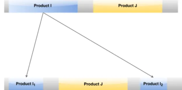
Fig.3. Conceptualinstanceofproductduplicationduetoproductiondiscruption.

PC= m i p Craw m ussmiTip (32) TC= m Craw m p i j=i

α

ij

Ttrans ijp +TF trans ijp_|p>1

+

β

ij

Zijp+ZFijp_|p>1

(33)

Overall, the decomposed iPSC model is an MILP and is formulated as follows:

Open−loopiPSC: maxPROF= RV−OC−IC−BC−PC−TC

Subjectto: Eqs.(1)–(18)

(

Planning−Scheduling

)

Eqs.(19)–(27)

(

Controlconsiderations

)

3.1.2. Open-loopiPSCwithreschedulingconsiderations

The decomposition of the iPSC through the use of linear metamodels and the offline derivation of the minimum transition times is valid under a number of deterministic assumptions throughout the three levels of integration. However, when dynamic disruptions are considered the need to account for possible reschedulings has to be addressed. To this end, the model presented in the previous section is modified accordingly. When dynamic disruptions are identified during the production of a product, it should be allowed to resume the production so as to attempt to fulfill the remaining demand. Product duplication is employed so as to facilitate this is- sue as shown in Fig. 3 .

Through product duplication, an identical product is created and inherits all the relevant information from the original one. Next a dynamic set is created, I I(i, j, p) which denotes the set of

products that are considered for duplication on a speciﬁc planning period, during which the disruption occurred. Moreover, the following sets are considered: I R(i) which is the set of only the orig-

inal products and I D(i, p) which is the set of the dummy prod-

ucts that represent the disturbance occurrence during period p. Eq. (34) is the modiﬁed version of Eq. (16) for the calculation of backlog, while for inventory calculations Eq. (17) is replaced by Eq. (35) .

Bcip=Bci,p−1+Dcip−Scip−

j∈II Scjp,

∀

c, i∈IR, p (34) Vip=Vi,p−1+Prip− c Scip+ j∈II Prjp− j∈II Scjp,

∀

i∈IR, p (35)

The minimum and maximum production times are relaxed for the case of disturbance modelling and thus Eq. (36) arises instead of Eq. (12) . Disturbances do not result production of products thus Eq. (37) is only employed for any product except for the ones that belong in I D

θ

lo

pEip≤Tip≤

θ

pupEip

∀

i / ∈ID, p (36)

(6)

Fig.4. NumericalintegrationofarbitrarytransitioncurveviaSimpson’srule.

Prip=riTip

∀

i / ∈ID, p (37)

As will be discussed in the next section, the closed-loop implementation of the iPSC is enabled via the use of novel multi- parametric controllers which communicate with the open-loop iPSC via a number of ways. One of them is via the information the controllers offer back to the integrated problem about the approximate transition cost between products in the case of rescheduling. In general the transition cost is the integral of the control actions (u(t)) over the transition period ( [0 ,T trans

ij ] ), i.e.,

Ttrans ij

0 u

(

t

)

dt . In or-

der to allow for fast calculations the controller is programmed to compute the numerical integral of the transition based on Simp- son’s rule which provides a good trade-off between numerical accuracy and computational expense as shown in Fig. 4 . Thus, the quantity CT ij

Ttrans ij

0 udt represents the numerical approximate

value of the transition cost as computed by the multi-parametric controller.

This results in the modiﬁcation of Eq. (33) about the calculation of the cumulative transition cost as shown in Eq. (38) .

TC= p i/∈ID j=i

α

ij

Ttrans ijp +Ttransijp_|p>1

+

β

ij

Zijp+ZFijp_|p>1

+ i∈ID j=i CTij

Zijp+ZFijp_|p>1

(38)

3.2.Closingtheloopviamulti-setpointexplicitnonlinearcontrollers 3.2.1. Multi-parametricmodelpredictivecontrol

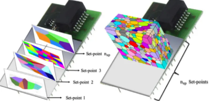
In this section we present the idea behind the design of multi- setpoint explicit controllers. Multi-parametric programming (mp-P) as an optimisation based methodology has found numerous ap- plications in the ﬁeld of process systems engineering with the design of explicit controllers probably being the most popular ( Charitopoulos and Dua, 2016; Dua et al., 2008; Oberdieck et al., 2016 ). Within the context of explicit MPC, one considers as uncertain parameters the initial states of the system at each sampling instance and thus an mp-P problem with uncertainty in the right hand side (RHS) of the constraints is formulated ( Bemporad et al., 2002 ). The solution of this mp-P problem leads to the computation of the control law, i.e. the optimal control input as explicit function of the state of the system together with the regions where each expression holds. Despite the fact that explicit MPC is one of the most well studied areas of mp-P theory, the design of explicit controllers for set-point tracking remains a rather diﬃcult task as one would have to design a controller for each set-point target given the methodologies that have been presented in the literature until now, especially for the nonlinear case ( Pistikopoulos et al., 2015 ).

Fig.5. Conceptualrepresentationofamulti-setpointexplicitcontroller.Ontheleft handsideaconventionalmulti-parametriccontrollerforvariousset-pointsis de-pictedwhileontherighthandsideamulti-setpointexplicitcontrollercanbe visu-alisedwiththethirddimensionbeingthecontinuousset-pointspace.

A generic mathematical formulation of the explicit MPC problem is given by Eq. (39) ,

⎧

⎪

⎨

⎪

⎩

(

x

(

tk

))

=min_u N−1 t=0 L

(

xt, ut

)

+E

(

xN

)

Subjectto: xt|t=0=x

(

tk

)

xt+1=f

(

xt, ut

)

t=0, 1, . . . , N−1 yt+1=h

(

xt

)

t=0, 1, . . . , N−1 g

(

xt, ut, yt

)

≤0 t=0, 1, . . . , N (39)

where xt, ut, yt are the state, control input and system output vec-

tors respectively at every sampling instance, t, and are n x, n u, n y

dimensional. Inequality constraints for the state, output and control inputs are represented without loss of generality by the vector function g∈Rng,_{the mappings}_h _:Rnx→Rny _and_f _:Rnx+nu→

Rnx _{correlate the output with the state and dictate the state evolu-}

tion of the system respectively. _L: _Rnx+nu_→_R_{is a stage cost and}

E : Rnx→R_{is a terminal cost function over the prediction hori-}

zon N. The repetitive solution of problem (39) provides the optimal cost

( x(t _k)) and the optimisation vector, which in this case is the sequence of optimal control inputs u∗=

u∗₁,u₂∗,...,u∗_N₋₁

over the ﬁnite prediction horizon N. While normally, the online repetitive solution of the receding horizon control problem is required, via the means of mp-P one can solve problem (39) for all possible realisations of the system’s measurements and thus compute oﬄine once and for all the optimal control law as a function of the system’s measurements, u=

δ

(

x_t_|_t₌₀

)

along with the corresponding critical regions (CRs), i.e. the parametric ranges over which each explicit expression is optimal.

The class of problems described in (39) involves uncertain parameters on the right hand side (RHS) of the constraints. When multiple set-points need to be considered then there are two ways of designing the explicit controller(s). The ﬁrst one, is to solve n sp mp-P problems, where n sp is the number of set-points con-

sidered and thus design n sp explicit controllers. The second al-

ternative, that we propose in the present work, is to design one multi-setpoint explicit controller (mp-MPC). The idea is to solve only one mp-P problem for n sp set-points and create a universal

“multi-layer” controller as shown conceptually in Fig. 5 .

Designing a multi-setpoint explicit controller mathematically can be expressed by Eq. (40) .

⎧

⎪

⎨

⎪

⎩

ϒ

(

x

(

tk

)

, xsp

)

=min u N−1 t=0 L

(

xt, ut, xsp

)

+E

(

xN, xsp

)

Subjectto: xt|t=0=x

(

tk

)

xt+1=f

(

xt,ut

)

t=0,1,...,N−1 yt+1=h

(

xt

)

t=0, 1, . . . , N−1 g

(

xt, ut, yt

)

≤0 t=0, 1, . . . , N xsp∈XSP (40)

(7)

The difference between problem (39) and problem (40) lies on the treatment of the set-points as uncertain parameters, which results in an mp-P problem with both RHS and objective function’s coeﬃcients (OFC) uncertainty. As seen in (40) , apart from the vector of the initial states ( x(t k)) the various set-points ( xsp) are con-

sidered as uncertain parameters as well. It is interesting to notice that, within the context of EWO, being able to design this kind of controllers is of great importance because the set-points targets are calculated dynamically by the decisions at the scheduling level. 3.2.2. Amethodologyforthedesignofmulti-setpointexplicit

controllers

As mentioned above we are interested in the following case: given a system that is required to operate at multiple set- points and the nonlinear terms involved in its model are non- transcendental we aim to design a single explicit controller that contains all the associated control laws. To do so, we employ con- cepts from computer algebra since the uncertain parameters are treated herein as symbolic expressions while the underlying optimisation problem is solved analytically using Gröbner bases theory ( Charitopoulos et al., 2017c; Dua, 2015 ). Gr ö bner bases theory emerged from the Ph.D. thesis of Bruno Buchberger as a way to analytically solve systems of polynomial multi-variable equations ( Buchberger, 2006 ). Briefly, Gröbner bases and the Buchberger algorithm can be seen as a generalisation of the Gaussian elimina- tion for the case of linear systems. Before we proceed further it is important to provide some formal definitions that are crucial in Gröbner bases theory.

Let k be any ﬁeld and let k[ x] =k[x 1,...,xt] be the ring of polynomials in t indeterminates. Any polynomial can be described as a sum of terms of the form:

α

x β1

1 · · ·x βtt with

α

∈k and

β

i∈N , i =

1 ,...,t and the term x β1

1 · · ·x βtt is called power−product.

Deﬁnition. (Gröbner basis ( Buchberger, 2006 )) A set of non-zero polynomials G ₌

{

g 1,...,g t

}

contained in an ideal I, is called a

Gröbner basis for I if and only if for all f ∈I such that f =0, there exists i ∈

{

1 ,...,t

}

such that lp(g i) divides lp(f), where lp( ·) stands

for the leading power-product of a polynomial function.

In the deﬁnition given, an ideal is a set of polynomials of the form t

i=1

u ig i with g i in G and arbitrary polynomials u i. The ex-

istence of such ideal is guaranteed by the Hilbert Basis theorem ( Bochnak et al., 2013 ), which also guarantees the termination of algorithms that are used for the computation of Gröbner bases. Roughly speaking, within Gröbner bases theory a set of polynomial V is transformed into an other set of polynomials G which is equivalent to the former but has certain favourable computational properties. At the core of Gröbner bases theory the Buchberger algorithm is found ( Buchberger, 2006 ) which is employed for the computation of the Gröbner basis of a speciﬁc set of polynomials. Buchberger introduced within the algorithm the concept of S- polynomials as well as provided a theorem for the proposed algorithm which for the sake of space are not discussed in the present article; however, the interested reader can refer to the book of book of Bochnak et al. (2013) . The implementation of the proposed methodology was done in Mathematica 11. The reason why computer algebra was chosen for the design of the multi-setpoint explicit controllers is because it provides us with the following degree of freedom. One can consider the various set-points as a single uncertain parameter bounded as shown by Eq. (41) .

xlosp≤xsp≤xupsp (41)

where x lo

sp, x upsp represent the lower and upper bounds on the set-

points set for the controller. However, within a computer algebra

environment, one can actually perform computations either in continuous or a discrete sets fashion as indicated by Eq. (42) . Thus following the methodology followed in the present work, the uncertain parameters involved in the mp-P problem for the design of the multi-setpoint explicit controller can be treated in either way.

xsp∈

x1 sp, x2sp, . . . , x nsp sp

(42)

Solving multi-parametric nonlinear programming problems (mp-NLPs) still remains a challenging task despite the research effort put in the literature of multi-parametric programming. Prob- lem (43) provides a generic mathematical formulation of mp- NLPs:

z

(

θ

)

=min

x f

(

x,

θ

)

Subjectto:g

(

x,

θ

)

≤0 (43)

x∈X⊆Rnx,

θ

∈

⊆_Rnθ

where x is the n x-vector of optimisation variables and belongs to

the bounded set X,

θ

is the n _θ−vector of uncertain parameters and belongs to the set

which may be unbounded. The function f and is a scalar-valued function and the function g is a vector-valued function of n g dimensions denoting the constraints of the optimi-

sation; note that both of the functionals mentioned can be linear or non-transcendental nonlinear. While a comprehensive review on the topic can be found in Domínguez et al. (2010) no previous work in the ﬁeld has presented an algorithm that can facilitate mp-NLPs with simultaneous variations on the RHS and the OFC. A considerable amount of research work has been devoted to the analytical solution of mp-NLPs using computer algebra principles ( Charitopoulos and Dua, 2016; Charitopoulos et al., 2017d; Dua, 2015; Fotiou et al., 2005 ) but only the case of RHS uncertainty has been treated. Recently, Charitopoulos et al. (2018) proposed an algorithm for the solution of mp-NLPs with non-transcendental nonlinear terms under the presence of simultaneous variations on RHS, left hand side (LHS) and OFC and this is the main machinery that is employed in the present work for the design of multi-setpoint explicit controllers.

They key idea of the aforementioned algorithm can be summarised as follows: given an mp-NLP, formulate the ﬁrst order KKT conditions and solve the resulting system of nonlinear equations using Gröbner Bases while treating the uncertain parameters as symbols. This step results in a set of candidate solutions for the optimisers x and the Lagrange multipliers

λ

which are parametric in

θ

and include: infeasible, local and global optima. For the candidate solutions computed, qualify with the primal and dual feasibility together with a constraint qualiﬁcation and remove the infeasible explicit solutions. Finally, perform a comparison procedure and keep only the globally optimal solutions along with their corresponding CRs, by computing the corresponding Cylindrical Al- gebraic Decompositions (CAD). For a detailed exposition the interested reader is referred to Charitopoulos et al. (2018) while a comprehensive overview on topics of Gröbner Bases Theory and CAD can be found in Bochnak et al. (2013) . It is worth to note that the proposed algorithm is dependent on Gröbner Bases calculations which have been proven to be doubly exponential with respect to the variables under determination in the worst case ( Charitopoulos et al., 2018; Fotiou et al., 2005 ). In Fig. 6 , an outline of the algorithm is presented.

3.3.Theoverallclosed-loopintegratedframework

Real processes are subject to a number of disturbances that endanger the feasibility and optimality of operations. For continuous manufacturing processes, fluctuations on the feed composi- tion, feed temperature as well as the flow rate of the reactants can lead to significant deviations from the desired open-loop state Please cite this article as: V.M. Charitopoulos et al., Closed-loop integration of planning, scheduling and multi-parametric nonlinear

(8)

Fig.6. Outlineofthemp-NLPalgorithm.

trajectory and result in the production of off-spec material. In the context of iPSC the different timescales involved, lead to the formulation of large scale MINLPs that pose an additional degree of complication that exacerbates the computational requirements and thus prohibit its online solution. In order to alleviate the computational complexity the proposed strategy involves an oﬄine step where linear metamodels that correlate the transition time and cost are built, along with the related nominal minimum transition times. By doing so, this aspect of the interdependence between scheduling and control is exploited and at the same time the control timescale is de-dimensionalised thus reducing the computational complexity. Furthermore, it can happen that the data provided about the transition time and cost from the optimal control simulations can lead to inconsistencies when compared to the closed-loop behavior of the system due to potential model mis-

match or because of the different objectives considered. To this end, the data used for the derivation of the linear metamodels as well as the minimum transition times are computed via a number of closed-loop simulations of the underlying dynamic system through the use of the multi-setpoint explicit controller that was introduced earlier. This was also done in order to simulate what would happen in a real process where the mechanisms that dictate the transition costs and times may not be suﬃciently captured by open-loop dynamic optimisation simulations but from historical data.

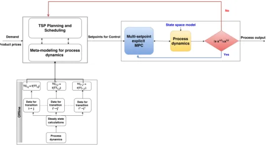
For the online part we consider the solution of an MILP (open- loop iPSC problem) and then the corresponding control problem that tracks online the open-loop solution. Conceptually, the proposed strategy for the closed loop solution is given in Fig. 7 .

Firstly, the mp-MPC for the underlying dynamic system is designed. As shown in Fig. 7 in an oﬄine step the linear metamodels that correlate transition time and cost are computed based on the closed-loop simulations of the system. The linear coeﬃcient of the metamodels are then used in the (open-loop iPSC) problem which is an MILP. The two parts (open-loop iPSC and (mps)- MPC) are coupled through the decision variables E ip, O ip and Z ijp,

ZF ijp. More speciﬁcally, the set of assigned products to the plan-

ning period is created and renewed in every planning period, i.e. Iactive

(

p

)

=

{

i

|

E ip=1

}

. Notice that every time a rescheduling takes

place the set of assigned products is revised accordingly. Next, the production sequence is made known to the controller through the integer variable O _ip and the binary variables that indicate the changeovers (Z ijp and ZF ijp) are employed for the derivation of

the desired set-points. In Algorithm 1 , an algorithmic chart for the integration of closed loop control is given. Initially a nominal production plan and the relevant schedules are computed by solving the open-loop iPSC ( Algorithm 1 , Step 1). The main computational loop iterates over all the planning periods under consideration ( Algorithm 1 , Step 2). The sequencing decisions and the set of assigned products are developed and then the schedule is supervised in a logic manner. A scalar k is used to track the order of the product that is currently being processed ( Algorithm 1 , Steps 3–6). Then following the proposed framework the information goes to the outer control loop where the mps-MPC is employed and the system is regulated around the desired set-point subject to the quality bound ( xq). If the system stays within this

limit ( Algorithm 1 , Step 10) then we sample the next instance normally; otherwise if the threshold/quality bound is violated that means that we have to ﬁx the products current production time, set the current measurement as the state of the disturbance and go

(9)

Algorithm1. Closed-loopiPSC.

to Algorithm 2 to initiate the rescheduling ( Algorithm 1 , Steps 10– 16). If the nominal production time has been accomplished without disruptions then we set the set-point of the mps-MPC as the steady state of the next product ( Algorithm 1 , Step 20) and start the changeover. Similar to the previous steps there has been set a threshold ( ) for which a disturbance during a transition is sup- posed to lead to negligible disruption and thus no rescheduling is triggered ( Algorithm 1 , Steps 21–33); otherwise a rescheduling needs to be initiated and the steps outlined in Algorithm 3 should be followed.

As shown in Algorithm 1 whether the disturbance is detected during a production or a transition period calls for different strate- gies. During the production period the role of control is to reg- ulate the system around the desired steady state given a quality bound for allowable deviation ( xq), which in the context of iPSC

reflects a specific product grade, while during the transition period there is a need for set-point tracking control. In the case that disturbance is detected during the production time of a product, it is assumed that its production is instantly interrupted as the disturbance exceeds the prespecified threshold ( ); note that in the present work we follow the convention of Zhuge and Ierapetri- tou (2012) and these parameters are assumed to be determined via heuristics based on process knowledge. Practically this hap- pens because in real processes there will always exist some noise and model-mismatch and without those tolerances there would be excessive need for rescheduling. Once the disturbance is detected during the production period, it is reasonable to consider

Algorithm2. Reschedulingroutineforproductiondisruption.

Algorithm3. Reschedulingroutinefortransitiondisruption.

the need of re-assignment of that product within the same planning period and this is achieved via a product duplication. The steps outlined in Algorithm 2 are then followed in order to decide upon the rescheduled optimal sequence that allows for resume of the production. That is, the current measurement of the system is assumed to be the steady state of a dummy product ( xss

d_name) and the mps-MPC is employed to simulate all the poten-

tial transitions to the other products and compute transition times and costs ( Algorithm 2 , Steps 1–14). Next, the set of products that have already been processed in the current period is constructed (I past) and the relevant timing and sequencing decisions are ﬁxed

( Algorithm 2 , Steps 15–17). Notice that by ﬁxing the timing de- Please cite this article as: V.M. Charitopoulos et al., Closed-loop integration of planning, scheduling and multi-parametric nonlinear

(10)

cisions, production decisions are also fixed given the assumption about constant production rate. Since the disruption was detected during a production period, it should be allowed to the model to choose the resume of production and to do so we follow the product duplication concept and define an alias element in the products set that is set to be active only for the current planning period and then we proceed in solving the reduce iPSC ( Algorithm 2 , Steps 19– 23). We employ the term “reduced iPSC” since the open-loop iPSC model is solved in reduced decision space, i.e. with the past decisions fixed.

Another case involves the disturbance detection and rejection during the transition time from one product to the other. In that case, there is no need to account for product duplication and we only introduce a new dummy product that represents the current state of the system after the disturbance is realised. Similar to Algorithm 2 , we exploit the ability of mp-MPC to run simulations in very fast times and the potential transition times and costs are computed ( Algorithm 3 , Steps 1–14). The output of these computations are passed to the model and the past decisions are ﬁxed ( Algorithm 3 , Steps 15–18) and the reduced iPSC is solved again to deﬁne the optimal rescheduling action ( Algorithm 3 , Steps 19–21). A summary of these steps is given in Algorithm 3 .

Overall, the integrated problem is formulated and solved as an MILP and the closed-loop is achieved through the rescheduling mechanism outlined in this section via the use of the proposed mp-MPC.

4. Casestudies

In this section the closed loop implementation of iPSC is illustrated through two case studies, where each planning period is assumed to be equal to one week. In all the case studies presented, it is assumed that every system exhibits multiple steady states at which a speciﬁc product is produced in a single CSTR while the occurrence of idle time results in the related start-up and shut- down requirements from a systems dynamics perspective. More- over, a short discussion on the results is conducted at the end of each case study. All the optimisation problems, are formulated and solved using GAMS 24.7.4, on a Dell workstation with 3.70 GHz processor, 16GB RAM and Windows 7 64-bit operating system using CPLEX 12.6.1 for the solution of the MILPs and BARON 16.8.24 ( Sahinidis, 1996 ) for the solution of NLPs. BARON was chosen for the comparison between the NLMPC and mp-MPC scheme because it is a global optimisation solver and the explicit solutions computed for the design of the mp-MPC controllers are globally optimal as well.

4.1.SingleinputsingleoutputCSTR

First, a case study involving a SISO multi-product CSTR is considered. Based on the concentration (C R) and the volumetric ﬂow

of the reactant (Q R) a number of products can be manufactured

at different steady state operating conditions; the related data are given in Table 1 . From the control perspective, the state variable of the system is the concentration of the reactant, while the control input is the volumetric ﬂow of the liquid. A conceptual representation of the related system is given in Fig. 8 . The reaction is 3 rd order irreversible, i.e. R→k 3 P, −RR=kCR3. The nonlinear dynamic model of the system is given by Eq. (44)

dCR

dt = QR

V

(

C0−CR

)

+RR (44)

where C 0 denotes the concentration of the reactant in the feed

stream, V is the reactor volume and k is the reaction’ s kinetic constant.

In order to design the multi-setpoint explicit controller the system’s model is transformed into its algebraic equivalent. In this

Table1

DataofSISOCSTRcasestudy. CostdataofSISOCSTR.

Product OCi(rmumol) Pi(rmumol)

A 0.13 200 B 0.22 150 C 0.35 130 D 0.29 125 E 0.25 120 F 0.18 180 G 0.27 124 H 0.29 140

DynamicdataofSISOCSTR. Product xss i(molL ) ussi(hL) A 0.0967 10 B 0.2 100 C 0.3032 400 D 0.393 1000 E 0.5 2500 F 0.15 39.7 G 0.45 1656.8 H 0.247 200.1

Fig.8. SISOCSTRproductionscheme,themanipulatedvariableisthevolumetric ﬂowrateoftheliquid(QR)whilethestatevariableistheconcentrationofthe

reac-tant(CR).

work, for the sake of simplicity an Euler integration scheme is followed and the problem is formulated as shown in Eq. (45) .

min u(t) J

(

θ

)

= tPH t=0

x

(

t

)

−xref

2 Subject to:

⎧

⎪

⎨

⎪

⎩

dx dt= u V

(

C0−x

)

+RR x

(

t

|

t=0

)

=

θ

1 xref₌

θ

2 0≤x

(

t

)

≤1, 0≤t≤tPH 0≤u

(

t

)

≤3000, 0≤t≤tPH (45)

For the design of multi-setpoint explicit controller the algorithm outlined in Section 3.2 was employed; the interested reader is referred to Charitopoulos et al. (2018) for a more detailed exposition on the main algorithmic steps. The mp-MPC was designed for prediction horizons of unity, two and three; the ﬁnal globally optimal explicit solutions along with their corresponding CRs are given in Table 2 while the ﬁnal partition of the parametric space is given in Fig. 9 . The corresponding explicit solutions are given in Table 3 . With regards to the computational behavior of the proposed scheme solving the corresponding mp-NLP for t PH=1

takes 22.65 s, t PH= 2 takes 262.43 s and t PH= 3 takes 2540.65 s.

As typically observed in the mp-P literature the computational effort grows rapidly with the number of variables and constraints ( Oberdieck et al., 2016 ).

Once the multi-setpoint explicit controller is designed we investigate its performance in comparison to the use of conventional MPC within the context of iPSC. First we consider the case of no imposed disturbances and then at speciﬁc time an additive distur-

(11)

Table2

FinalCRsandexplicitsolutions(controllawandstateevolution)fortPH=1fortheSISOCSTRcasestudy.

CRs Mathematicalexpression Explicitsolution

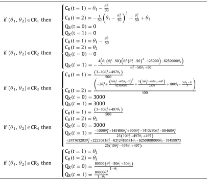
CR1:= θ2≥0.0967 ⎧ ⎪ ⎪ ⎪ ⎨ ⎪ ⎪ ⎪ ⎩ 0.096718≤θ1≤0.503 0.02θ3 1+θ2≤θ1 0.503≤θ1≤1 θ2≤0.5 CR(t=1)=θ1−θ 3 1 50 QR(t=0)=0 CR2:= θ2≤0.5 ⎧ ⎪ ⎪ ⎪ ⎪ ⎪ ⎨ ⎪ ⎪ ⎪ ⎪ ⎪ ⎩ θ2≥0.0967 θ1=1 0≤θ1≤0.09126 0.09126≤θ1≤0.4994 0.994θ1+0.006≤0.02θ13+θ2 0.0967≤θ2 0≤θ1≤0.09126 CR(t=1)=( 3−10θ3 1+497θ1) 500 QR(t=0)=3000 CR3:= ⎧ ⎪ ⎪ ⎪ ⎪ ⎪ ⎪ ⎪ ⎪ ⎪ ⎨ ⎪ ⎪ ⎪ ⎪ ⎪ ⎪ ⎪ ⎪ ⎪ ⎩ 0.0913<θ1≤0.0967 0.0967≤θ2≤0.002(3+497θ1−10θ13) 0.499≤θ1≤0.503 0.0250θ1−θ13 ≤θ2≤0.5 0.0967≤θ1≤0.4994 0.0250θ1−θ13 ≤θ2≤0.002 −10θ3 1+497θ1+3 CR(t=1)=θ2 QR(t=0)= 10000(θ3 1−50θ1+50θ2) 1−θ1

Fig.9. OptimalpartitionoftheparametricspacefortheSISOCSTRcasestudy.

Table3

FinalexplicitoptimalsolutionsfortPH=2fortheSISOCSTRcasestudy.

if(θ1,θ2)∈CR1then ⎧ ⎪ ⎪ ⎪ ⎨ ⎪ ⎪ ⎪ ⎩ CR(t=1)=θ1−θ 3 1 50 CR(t=2)=−501 θ1−θ 3 1 50 3 −θ3 1 50+θ1 QR(t=0)=0 QR(t=1)=0 if(θ1,θ2)∈CR2then ⎧ ⎪ ⎪ ⎪ ⎨ ⎪ ⎪ ⎪ ⎩ CR(t=1)=θ1−θ 3 1 50 CR(t=2)=θ2 QR(t=0)=0 QR(t=1)=− 4θ1(θ12−50) θ2 1(θ12−50) 2 −125000−6250000θ2 θ3 1−50θ1+50 if(θ1,θ2)∈CR3then ⎧ ⎪ ⎪ ⎪ ⎪ ⎨ ⎪ ⎪ ⎪ ⎪ ⎩ CR(t=1)=( 3−10θ3 1+497θ1) 500 CR(t=2)= −2θ3 1+( 10θ3 1−497θ1−3)3 62500000 + 3(10θ3 1−497θ1+497) 2500 +100θ1− 3(θ1−1) 5 100 QR(t=0)=3000 QR(t=1)=3000 if(θ1,θ2)∈CR4then ⎧ ⎪ ⎪ ⎪ ⎪ ⎪ ⎨ ⎪ ⎪ ⎪ ⎪ ⎪ ⎩ CR(t=1)=( 3−10θ3 1+497θ1) 500 CR(t=2)=θ2 QR(t=0)=3000 QR(t=1)=−1000θ 9 1+149100θ17+900θ16−7410270θ51−89460θ14 25(10θ3 1−497θ1+497) +247763203θ3 1+2223081θ21−6212486581θ1+6250000000θ2−37499973 25(10θ3 1−497θ1+497) if(θ1,θ2)∈CR5then ⎧ ⎪ ⎪ ⎨ ⎪ ⎪ ⎩ CR(t=1)=θ2 CR(t=2)=θ2 QR(t=0)= 10000(θ3 1−50θ1+50θ2) 1−θ1 QR(t=1)=10000θ 3 2 1−θ2

(12)

Fig.10.ComparisonoftheclosedloopbehaviorofthestateoftheSISOCSTR(CR)

usingexplicitMPC(bluecontinuousline)andconventionalMPC(reddashedline) forpredictionhorizonofunity(1stplanningperiod).(Forinterpretationofthe ref-erencestocolourinthisﬁgurelegend,thereaderisreferredtothewebversionof thisarticle.)

bance is imposed and the dynamic behavior of the closed loop system is evaluated.

4.1.1. Case1:Noadditivedisturbanceimposed

First the closed loop behavior for prediction horizon of unity and then two is evaluated for the mp-MPC, the threshold values are set to

ω

=10 −6_, ₌_±_{5% and no imposed additive disturbance}

is considered, while a planning horizon of two weeks is employed. When the mps-MPC is employed, it takes 0.1705 CPU s for the nominal iPSC solution to be computed. For the case of the conventional NLMPC the same results are computed at 291.92 CPU s, a rather considerable difference in terms of computational effort. It is important to note that based on Fig. 10 , the dynamic response of the system as computed by the mp-MPC and the conventional NLMPC are identical.

The same instance of the case study was investigated, by em- ploying prediction horizon of 2 for both the explicit and the conventional MPC schemes. Regarding the dynamic response and the stability of the underlying control system, the results indicate no difference when compared to the ones computed for prediction horizon of unity. As far as the online computational complexity is concerned, for the case of the multi-setpoint explicit MPC it takes 0.1707 s for the whole iPSC to be solved and validated in a closed loop manner while the same problem takes 831.24 s using the conventional MPC using BARON 16.3.4 and optimality tolerance of 10 −5_.

As mentioned earlier in the article, real process systems are subject to a number of disturbances that may affect signiﬁcantly the performance of the process. For the case that no disturbances are accounted for, the solution of the open loop and the closed loop iPSC are identical as demonstrated in case 1. However, under the effect of disturbances the need of feedback control mechanism becomes crucial. In the next two cases we investigate the effect of the implementation of the closed-loop strategy under the occurrence of disturbances that lead to state deviation.

4.1.2. Case2:Statedeviationduringthetransitionperiod

In this case we assume that the nominal iPSC has been solved and the optimal decisions begin to be applied to the plant. During

Fig.11. Comparativeplotofthestatedeviationduringthetransitionperiod.

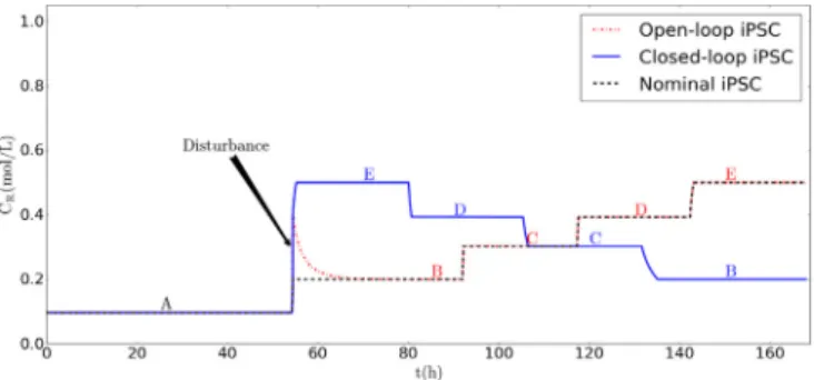
the first planning period, a disturbance is detected 12 minutes after the beginning of the transition from product A to product B and its magnitude exceeds the prespecified threshold. The rescheduling mechanism is triggered and first the current state of the system is passed to the mp-MPC according to the steps outlined in Algorithm 3 . It takes 0.008s for the mp-MPC to compute the candidate transition times and costs which are subsequently passed to the iPSC rescheduling model in order to compute the next optimal step. In this instance, the rescheduling mechanism dictates the change in the nominal sequence and instead of B the system is driven to the production of E while the production of B is set to be the last of the planning period. A graphical representation of this instance is given in Fig. 11 .

On the other hand, if the iPSC solution was applied without any feedback mechanism that would effectively close the loop, the pre- computed nominal control would have been applied to the system regardless of the disturbance occurrence. The impact of the disturbance on the open-loop framework was simulated by ﬁxing all the relevant decisions and as shown in Fig. 11 , it results in signiﬁcantly extended transition time from product A to B which results in turn in considerable reduction of the production time and thus increase in the backlog of the corresponding unmet demand. A summary of the results is given in Table 4 .

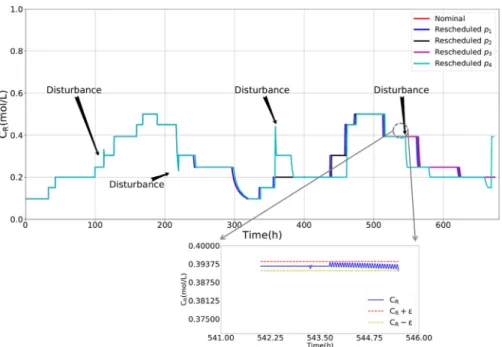
4.1.3. Case3:Multipledisturbancesovertheplanninghorizon In this case we consider 8 products and 4 planning periods. Solving the nominal problem, no disturbance is assumed and it takes 9.984 s for CPLEX 12.6.3 to compute the optimal solution. Within the ﬁrst planning period, during the transition from H to C, 4.2 min after the transition has started (nominal transition time is 6.6 min), a state deviation is realised which exceeds the threshold and is equal to 0.04 mol

L resulting in a concentration of 0.329 molL ,

after its realisation the proposed framework is employed and the need for rescheduling is examined. First, the explicit controller is used for a simulation between all the remaining products of the set Iactive( p) and then the reduced iPSC is solved (7.083 s) for the remainder of the planning horizon. In this case, the optimal solution dictates that it is preferable to keep on the prolonged transition rather than switching production to another product. The result of the extended transition is the decrease of production time of product G and its subsequent increase during planning period 2.

Table4

ComparativeresultsforthesolutionscomputedbytheclosedloopiPSCandtheopenloopiPSC.

Openloopnodisturbance Closedloopwithdisturbance Openloopwithdisturbance iPSCsolution A→B→C→D→E A→E→D→C→B A→B→C→D→E

E→C→B→A B→A→C→E E→C→B→A Proﬁt(rmu) 9.18·106 _9.174_·₁₀6 _8.65_·₁₀6

Backlogcost(rmu) 62331.9 68729.1 338677.65 TotalCPU(s) 0.152(mp-MPC)/ 0.27(mp-MPC) 0.152(mp-MPC)

(13)

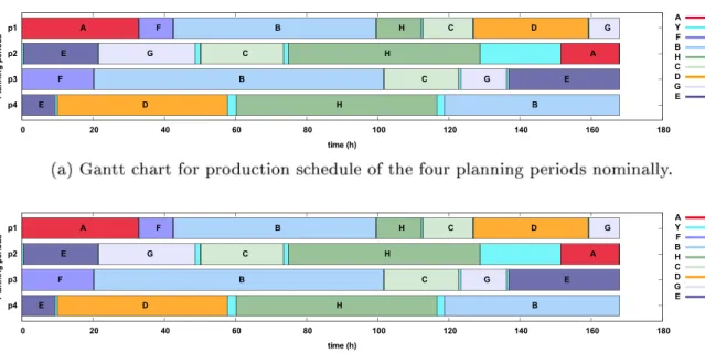
Fig.12. Ganttchartsoftheclosed-loopiPSCfortheSISOCSTRcasestudy.Thehorizontalaxisrepresentthetime(h)andeachweekspansacross168hwithchangeovers indicatedusingthe“Y” label.

Moving on to period 2, another dynamic disruption is realised during the transition from G to C (after 1.4 h of its start) and the system is led to x _d

2=0 .2306

mol

L . Following Algorithm 1 , this mea-

surement is passed to mp-MPC for the calculation of the potential transition times and costs. This instance of the closed-loop integration in quite interesting as the rescheduling mechanism for the current planning period generates a completely different solution for the remaining iPSC and this can be visualised in Gantt chart that is given in Fig. 12 .

As shown in Fig. 12 the disruption results in decrease of production of product C that in order to be rectiﬁed the sequencing decisions in planning period p 3 were revised. Finally, during pe-

riod 4, the case of dynamic disruption during production period is examined. While product D is being produced there is a dis-

crepancy in the system’s dynamics. Due to this discrepancy during the production period the steps outlined in Algorithm 2 are followed and a duplicate product of D is created and the reduced iPSC is solved again with ﬁxed the past decisions. As shown also in Fig. 12 , it was computed that the optimal corrective move would be to return in the production of D. A graphical interpretation of the system’s dynamics throughout the 4 planning periods is given in Fig. 13 , where also the last rescheduling instance is illustrated in more details.

4.2.Methyl-methacrylatepolymerisationreactor

Next the closed-loop iPSC of an isothermal methyl-methacrylate (MMA) polymerisation CSTR is studied. The free radical polymeri- Please cite this article as: V.M. Charitopoulos et al., Closed-loop integration of planning, scheduling and multi-parametric nonlinear

(14)

Fig.13. CR=f(t)plotindicativeofthesystem’sdynamicsovertheentireplanninghorizon.

Table5

DecisionvariablesoftheMMAkineticmodel.

Cm(kmol_m3 ) State:concentrationofmonomer

Cl(kmolm3 ) State:concentrationofinitiator

D0(kmolm3 ) State:deadchainsmolarconcentration

Dl(mkg3) State:deadchainsmassconcentration

Fl(m

3

h) Input:ﬂowrateofinitiator

y=Dl/D0(kmolkg ) Output:molecularweight

Table6

KineticdatafortheMMApolymerisationreactor. F=10.0m3_/_h _Monomer_ﬂowrate

V=10.0m3 _Reactor_volume

f∗₌₀_.₅₈ _Initiator_eﬃciency

kp=2.50×106 m

3

kmol·h Propagationrateconstant

kTd=1.09×1011 m

3

kmol·h Terminationbydisproportionation

Rateconstant kTc=1.33×1010 m

3

kmol·h Terminationbycoupling

Rateconstant Clin=8.00kmol/m

3 _Inlet_initiator_{concentration}

Cmin=6.00kmol/m

3 _Inlet_monomer_{concentration}

kfm=2.45×103 m

3

kmol·h Chaintransfertomonomerrateconstant

kl=1.02×10−1h−1 Initiationrateconstant

Mm=100.12kg/kmol Molecularweightofmonomer

sation reaction takes place in an isothermal CSTR at the temperature of 335K, where MMA is produced using azobis (isobutyroni- trile) as initiator and toluene as solvent. The mathematical model is adopted from Chu and You (2012) and is given by Eqs. (46) –(50) . The system involves 4 state variables, i.e. the concentration of the monomer (C m), the concentration of the initiator (C l), the molar

concentration of the dead chains (D 0) and the mass concentration

of the dead chains (D l), one control input, i.e. the ﬂowrate of the

initiator (F l) and one output, i.e. the molecular weight of the poly-

mer produced (y). Based on different steady states that the system exhibits it is possible to produce different polymeric grades which correspond to different molecular weights and each grade forms a product within the iPSC framework. The notation used in the present case study is given in Table 5 , while the values of kinetic parameters are given in Table 6 .

dCm dt =−

(

kp+kfm

)

2f∗_k_l_C_l kTd+kTc Cm+ F

(

Cmin−Cm

)

V (46) Table7

SteadystateinformationaboutthedifferentpolymergradesoftheMMACSTRcase study. Product Css m Cssl Dss0 Dssl Yss Fssl A 3.2285 0.1216 0.0163 277.47 17,000 0.1675 B 3.0780 0.1487 0.0195 292.54 15,000 0.2049 C 3.3667 0.1009 0.0138 263.64 19,000 0.1391 D 3.3331 0.1056 0.0144 261.01 18,500 0.1455 E 3.4635 0.0885 0.0123 253.95 20,500 0.1219 F 3.5552 0.0780 0.0111 244.76 22,000 0.1075 G 3.7257 0.0615 0.0091 227.69 25,000 0.0847 H 3.8815 0.0491 0.0075 212.09 28,000 0.0677 I 3.9786 0.0426 0.0067 202.38 30,000 0.0587 J 4.1154 0.0346 0.0057 188.68 33,000 0.0476 K 4.2015 0.0302 0.0051 180.06 35,000 0.0416 L 4.3238 0.0248 0.0044 167.81 38,000 0.0341 M 4.4013 0.0217 0.0040 160.05 40,000 0.0299 N 4.4760 0.0191 0.0036 152.57 42,000 0.0263 O 4.5302 0.0173 0.0033 147.15 43,500 0.0239 P 4.5830 0.0157 0.0031 141.86 45,000 0.0217 dCl dt = FlClin−FCl V −klCl (47) dD0 dt =

(

0. 5kTc+kTd

)

2f∗_k_l_C_l kTd+kTc Cm+kf m

2f∗_k_l_C_l kTd+kTc Cm− FD0 V (48) dDl dt =Mm

(

kp+kfm

)

2f∗_k_l_C_l kTd+kTc Cm− FDl V (49) y= Dl D0 (50)

In order to demonstrate the merits of the proposed framework we assume that there are 16 polymer grades that can be produced and their corresponding steady state information are given in Table 7 ; notice that for the sake of space the values are given with truncated decimal points while for the numerical calculation the precision was up to 10 decimal places.

(15)

Table8

EconomicdataoftheMMAcasestudy.

Product OCi[rmukg] Pi[rmukg] ri[kgh]

A 263 388.5 100.529 B 188 252.8 122.937 C 163 247.8 83.457 D 226 293 87.325 E 220 330.5 73.165 F 210 260 64.504 G 190 290 50.833 H 240 350 40.635 I 230 395 35.214 J 290 325 28.607 K 205 310 24.997 L 210 316 20.500 M 183 220 17.996 N 155 260 15.814 O 149 300 14.359 P 134 324 13.040 Table9

ComputationalstudyofCPU(s)fordifferentpredictionhorizonsusingBARONwith zerorelativeoptimalitygap.

Hp CPU(s) 1 602.676 2 1905.328 5 3600a 10 3600a 20 3600a

a _The_solver_failed_to_converge_within₃₆₀₀_s.

Table10

Uncertainparametersofmps-MPCfortheMMACSTRcasestudy. Uncertainparameter Bounds Correlation

θ1 ∈[0,5] Cm|t=0 θ2 ∈[0,0.5] Cl|t=0 θ3 ∈[0,0.05] D0|t=0 θ4 ∈[0,300] Dl|t=0 θ5 ∈[0,5] Set-pointsforCm θ6 ∈[0,0.5] Set-pointsforCl θ7 ∈[0,0.05] Set-pointsforD0 θ8 ∈[0,300] Set-pointsforDl With regards to the economic data a summary of the selling prices and costs is given in Table 8 while inventory and backlog costs are calculated as 10% and 30% of the product’s selling price, P i.

Since none of the nonlinear terms in the system is transcendental, the proposed methodology for the design of the explicit controller can be employed. More specifically, the infinite dimensional optimal control problem is transformed into a finite one with the employment of a discretisation scheme. The present case study has been studied by a considerable number of researchers and it has been reported that its optimal control through numerical schemes is rather challenging due to numerical instabilities that may arise during the discretisation. To this effect, the most common discretisation scheme used is orthogonal collocation on finite elements because of its inherent properties of numerical stability. However, in the present work we employed forward Euler discretisation with a step size of h e=0 .01 h as trade-off between computational com-

plexity and stability of the integration scheme. A number of simulations were conducted so as to decide on a step size that can be small enough so as to avoid oscillatory behavior but not too small so as to avoid an extenuating repetitive solution that would result in further computational effort. Moreover, as will be shown in the results the nature of proposed methodology, i.e. the analytical and not numerical solution of the mp-MPC problem, enhances the ro- bustness of the solutions computed as numerical instabilities were circumvented.

Following the proposed methodology, ﬁrst the set of differential equations involved in the problem is discretised and then the parametric optimisation problem is formulated and solved in Mathe- matica 11. At this point, the prediction horizon was set to be equal to unity as from oﬄine simulations the enhancement of the controller’s stability was not highly affected. On the contrary, following the proposed methodology the global optimality of the explicit solutions is guaranteed whereas using readily available numerical solvers for online implementation of globally optimal solutions results in rather exhaustive computational times given the need for rapid solutions within the context of iPSC. For illustration purposes the results of a comparative study using BARON 16.8.24 solver in GAMS with varying prediction horizons is provided in Table 9 .

In order to design the explicit controller we consider 8 uncertain parameters, 4 for each state and 4 for each family of set- points. From previous experience within our group the number of uncertain parameters considered does not affect the computational complexity of the solution procedure as the uncertain parameters are treated in a symbolic way. In Table 10 , the notation for the uncertain parameter introduced in the present example is given. Note that the bounds on the uncertain parameters regarding the set-points are continuous. It can be argued that having these parameters as continuous may lead to unnecessary computations but one could argue that in the context of enterprise wide optimisation where the supervisory controller receives data from the RTO layer the constant use of the same set-points is not guaranteed. In that case a conventional explicit controller would have to be re- designed from the beginning (solution of the corresponding mp-P problem, storage of the explicit solutions, possibly, in a micro-chip) whereas following the methodology proposed herein, there would be no need for that, under the assumption that the bounds used initially are the feasible range of the system.

The corresponding mp-NLP problem consists of one optimisation variable, the control input, ten constraints and eight uncertain parameters. Note that even though the optimisation variable is one, the variables for which we seek analytical solution are eleven, i.e. the optimisation variable and the Lagrange multipliers of the constraints. Solving the mp-NLP results in 5 candidate solutions which are shown in Table 11 . An interesting observation is that the underlying control law is lin