Learning Latent Characteristics of Data and Models using Item Response Theory

(1)

University of Massachusetts Amherst University of Massachusetts Amherst

ScholarWorks@UMass Amherst

Doctoral Dissertations Dissertations and Theses

March 2020

Learning Latent Characteristics of Data and Models using Item

Response Theory

John P. Lalor

University of Notre Dame

Follow this and additional works at: https://scholarworks.umass.edu/dissertations_2

Part of the Artificial Intelligence and Robotics Commons

Recommended Citation Recommended Citation

Lalor, John P., "Learning Latent Characteristics of Data and Models using Item Response Theory" (2020). Doctoral Dissertations. 1842.

https://scholarworks.umass.edu/dissertations_2/1842

This Open Access Dissertation is brought to you for free and open access by the Dissertations and Theses at ScholarWorks@UMass Amherst. It has been accepted for inclusion in Doctoral Dissertations by an authorized administrator of ScholarWorks@UMass Amherst. For more information, please contact

(2)

LEARNING LATENT CHARACTERISTICS OF DATA

AND MODELS USING ITEM RESPONSE THEORY

A Dissertation Presented by

JOHN P. LALOR

Submitted to the Graduate School of the

University of Massachusetts Amherst in partial fulfillment of the requirements for the degree of

DOCTOR OF PHILOSOPHY February 2020

(3)

c

(4)

LEARNING LATENT CHARACTERISTICS OF DATA

AND MODELS USING ITEM RESPONSE THEORY

A Dissertation Presented by

JOHN P. LALOR

Approved as to style and content by:

Hong Yu, Chair

James Allan, Member

Brendan O’Connor, Member

Lisa Keller, Member

James Allan, Chair of the Faculty

(5)

DEDICATION

(6)

Ad maiorem Dei gloriam

St. Ignatius of Loyola

I bpoll sa talamh a bh´ı c´ona´ı ar hobaid

(7)

ACKNOWLEDGMENTS

This is the part where I thank everyone who made this possible.

I have to start with my advisor, Hong Yu. Throughout my time at UMass, you have supported me, encouraged me, and, most importantly, challenged me. I’ve learned so much from you during my time at UMass. To my dissertation committee, James Allan, Brendan O’Connor, and Lisa Keller, thank you for the very helpful input and suggestions throughout this process. Your help has only improved what is presented here. Hao Wu, Kathy Mazor, and Bev Woolf have been wonderful collaborators for several research projects. Their guidance and suggestions have helped strengthen all of the work presented here. The members of the BioNLP lab have been sounding boards, cheerleaders, and friends, among other things. Abhyuday, Jesse, Jiaping, Subhendu, Bhanu, Frank, Alice, Tsendee, Jinying, Emily, Elaine, Weisong, Kathryn, and everyone else, thank you all. Thank you to everyone at CICS, especially Leanne LeClerc and Eileen Hamel.

Before I started at UMass I was a part-time Masters student at DePaul taking a full-time course load. It was there that I first thought of research as a career, and I must thank the great professors at DePaul who worked with me to develop that interest and expose me to several different areas within CS: Amber Settle, Terrie Steinbauch, Craig Miller, Robin Burke, Jonathan Gemmell. To Rob Easley and everyone in the Mendoza College of Business at Notre Dame, that is where it all started for me, and I am so excited to be returning.

During my Ph.D. I had the opportunity to spend summers working at ESPN and Amazon. For a life-long athlete, getting to see how the sausage was made in

(8)

Bristol, CT really was a dream come true. To Zvi Topol, Javid Husenov, Adithya Tammavarapu, Sean Sanders, Segun Oshin, and everyone in the ESPN Advanced Technology Group who made that a very enjoyable and productive summer, thank you. Imre Kiss, Bill Campbell, Eunah Cho, Francois Marrissee and the rest of the Alexa team in Cambridge, MA pushed me to take what I’d learned and put it into practice, while also thinking through new research ideas.

When I was young, there was a rule in my house with regards to books: you can have them. Mom and Dad, you have always supported me and my interests. You pushed me when I was young to stay focused and challenge myself, in all aspects of life. Thank you. Kevin, you are and have always been my best friend. I can talk to you about anything, and spending time with you and your wife (!) Meghan on trips home to Philly has always been a great way to unwind and leave the stresses of work behind.

I would not be here if it weren’t for the love and support of my wife Kaitlin. From Notre Dame to Chicago to Western Mass. and back to ND, you have been my rock, my support, and my inspiration. During the highs and lows and stresses and more stresses of this process, you have always been there for me. I love you.

I dedicate this thesis to our girls, Teresa and Maeve, and to our upcoming third child. Tess and Maeve, watching you grow and learn has been the greatest experience of my life. I can’t wait to see the women that you become. BL3, we’re very excited to meet you in March!

(9)

ABSTRACT

LEARNING LATENT CHARACTERISTICS OF DATA

AND MODELS USING ITEM RESPONSE THEORY

FEBRUARY 2020

JOHN P. LALOR

B.B.A., UNIVERSITY OF NOTRE DAME M.Sc., DEPAUL UNIVERSITY

Ph.D., UNIVERSITY OF MASSACHUSETTS AMHERST

Directed by: Professor Hong Yu

A supervised machine learning model is trained with a large set of labeled training data, and evaluated on a smaller but still large set of test data. Especially with deep neural networks (DNNs), the complexity of the model requires that an extremely large data set is collected to prevent overfitting. It is often the case that these models do not take into account specific attributes of the training set examples, but instead treat each equally in the process of model training. This is due to the fact that it is difficult to model latent traits of individual examples at the scale of hundreds of thousands or millions of data points. However, there exist a set of psychometric methods that can model attributes of specific examples and can greatly improve model training and evaluation in the supervised learning process.

Item Response Theory (IRT) is a well-studied psychometric methodology for scale construction and evaluation. IRT jointly models human ability and example character-istics such as difficulty based on human response data. We introduce new evaluation

(10)

metrics for both humans and machine learning models build using IRT, and propose new methods for applying IRT to machine learning-scale data.

We use IRT to make contributions to the machine learning community in the following areas: (i) new test sets for evaluating machine learning models with respect to a human population, (ii) new insights about how deep-learning models learn by tracking example difficulty and training conditions, and (iii) new methods for data selection and curriculum building to improve model training efficiency, (iv) a new test of electronic health literacy built with questions extracted from de-identified patient Electronic Health Records (EHRs).

We first introduce two new evaluation sets built and validated using IRT. These tests are the first IRT test sets to be applied to natural language processing tasks. Using IRT test sets allows for more comprehensive comparison of NLP models. Second, by modeling the difficulty of test set examples, we identify patterns that emerge when training deep neural network models that are consistent with human learning patterns. Specifically, as models are trained with larger training sets, they learn easy test set examples more quickly than hard examples. Third, we present a method for using soft labels on a subset of training data to improve deep learning model generalization. We show that fine-tuning a trained deep neural network with as little as 0.1% of the training data can improve model generalization in terms of test set accuracy. Fourth, we propose a new method for estimating IRT example and model parameters that allows for learning parameters at a much larger scale than previously available to accommodate the large data sets required for deep learning. This allows for learning IRT models at machine learning scale, with hundreds of thousands of examples and large ensembles of machine learning models. The response patterns of machine learning models can be used to learn IRT example characteristics instead of human response patterns. Fifth, we introduce a dynamic curriculum learning process that estimates model competency during training to adaptively select training data that is appropriate

(11)

for learning at the given epoch. Finally, we introduce the ComprehENotes test, the first test of EHR comprehension for humans. The test is an accurate measure for identifying individuals with low EHR note comprehension ability, and validates the effectiveness of previously self-reported patient comprehension evaluations.

(12)

LIST OF TABLES

Table Page

2.1 Summary statistics from the AMT HITs. . . 34 2.2 Fleiss’κ scores for the NLI and SA annotations collected from AMT.

Original label-level agreement scores for SNLI are also reported. Inter-annotator agreement was not reported during SSTB

collection. . . 35 2.3 Examples of retained & removed sentence pairs. The selection is not

based on right/wrong labels but based on IRT model fitting and example elimination process. Note that no 4GS entailment

examples were retained (Section 2.2.6) . . . 37 2.4 Parameter estimates of the retained examples . . . 39 2.5 Theta scores and area under curve percentiles for LSTM trained on

SNLI and tested onGSIRT. We also report the accuracy for the

same LSTM tested on all SNLI quality control examples (see Section 2.2.2). All performance is based on binary classification for each label. . . 42 2.6 Estimated ability (θ) and held-out test set accuracy for two LSTM

models trained with a full training set (M1) and a sampled training data set (M2). Differences in θ are larger than differences in

accuracy and better indicate the gap in model performance. . . 44 3.1 Examples of sentence pairs from the SNLI data sets, their

corresponding gold-standard label, and difficulty parameter (bi) as

measured by IRT (§2.1). . . 47 3.2 Examples of phrases from the SSTB data set, their corresponding

gold-standard label, and difficulty parameter (bi) as measured by

IRT (§2.1). . . 47 3.3 Theta Percentile Scores of tested models on the full SNLI training set.

(18)

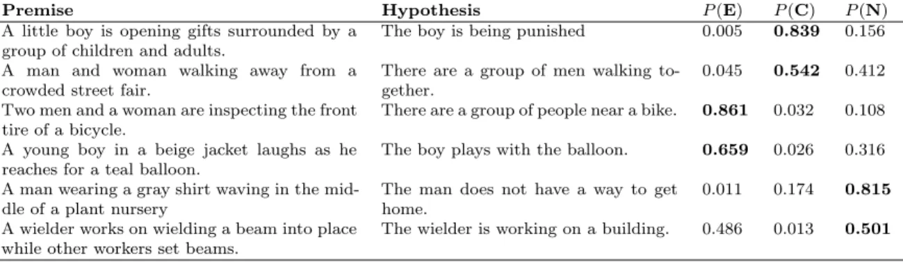
4.1 Examples of premise-hypothesis pairs from the SNLI data set and the AMT-estimated probability that the correct label is Entailment (E), Contradiction (C), or Neutral (N). The original gold-standard

label from SNLI is in bold. In some cases, the gold label provided originally has a low probability based on AMT-population

estimates (i.e. less than 75%). . . 68 4.2 Examples from the SSTB data set and the AMT-estimated

probabilities over labels. The gold label from SSTB is in bold. . . 68 4.3 Training and test accuracy results for incorporating SLMG in three

tasks: NLI, binary sentiment analysis (SA-B), and fine-grain sentiment analysis (SA-FG). Note: for B2, we cannot run on the fine-grained sentiment analysis task because the supplemental data set only includes binary sentiment labels (positive/negative). . . 72 4.4 Examples of premise-hypothesis pairs from the SNLI data set and

output probabilities from the LSTM model. For both examples the probabilities associated with the gold label are in bold. . . 73 4.5 Confusion matrices for the LSTM model, trained according to the

baseline (first block), using SLMG-S with CCE (second block), and using SLMG-S with MSE (third block). Gold standard labels run down the left hand side, while predicted labels are across the top in the matrix. The highest count of True Positives for each label

across the three model-training setups are in bold. . . 74 5.1 Dev accuracy results for MT-DNN model with different training set

sampling strategies. . . 94 5.2 The easiest and hardest examples judged by machine responses for

each class in the SNLI test data set. . . 95 5.3 Examples from the SNLI and SSTB data sets where the ranking in

terms of difficulty varies widely between human and DNN models. In all cases difficulty is ranked from easy to hard (1=easiest). . . 96 6.1 Percent change in training size (lower is better) and test set accuracy

(higher is better) for each curriculum learning method tested. . . 113 6.2 Examples from SSTB with the largest differences in difficulty. . . 114 6.3 Examples from SSTB with the largest differences in difficulty. . . 114

(19)

7.1 Example of questions generated from the researcher/physician

groups. . . 124 7.2 Examples of how the generated questions would be displayed as a

questionnaire, using the example from Table 7.1. . . 124 7.3 Demographic information of Turkers from the per-topic and validation

AMT tasks. a_{Age demographic information was not collected as}

part of the per-topic AMT tasks. . . 128 7.4 Average estimated ability of Turkers according to demographic

information for the validation task. . . 129 7.5 Examples of retained and removed questions following IRT

analysis. . . 130 7.6 Demographic information of Turkers from the follow-up study. . . 142 7.7 Mean scores for the 3 groups. Mean NoteAid scores are significantly

higher than the mean baseline scores, both for raw scores (P = .01) and estimated ability (P =.02). . . 145

(20)

LIST OF FIGURES

Figure Page

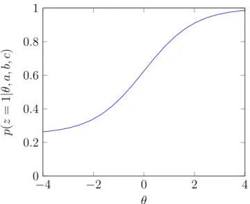
1.1 Example ICC for a “good” example, fit as part of a 3PL Model. For

this example, ai = 1, bi = 0, and ci = 0.25. . . 12

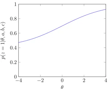
1.2 Example ICC for a “bad” example, fit as part of a 3PL Model. For

this example, ai = 0.5, bi = 0, and ci = 0.4. . . 13

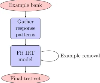
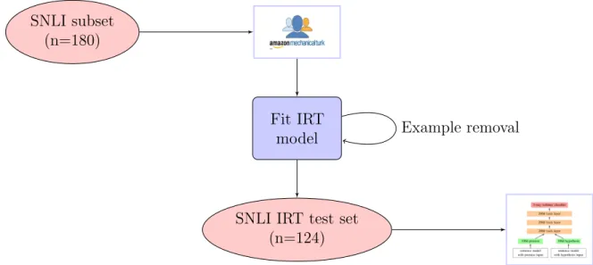
2.1 High level overview of the test set construction process with IRT. . . 31 2.2 Building an IRT test set for the SNLI data set. Response patterns

were obtained from Amazon Mechanical Turk workers (Turkers) and processed using IRT. A subset of examples were retained following analysis as the final test set. The test set can then be

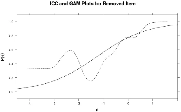
administered to a trained DNN model. . . 32 2.3 Estimated (solid) and actual (dotted) response curves for a removed

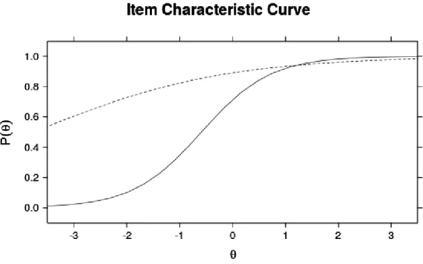
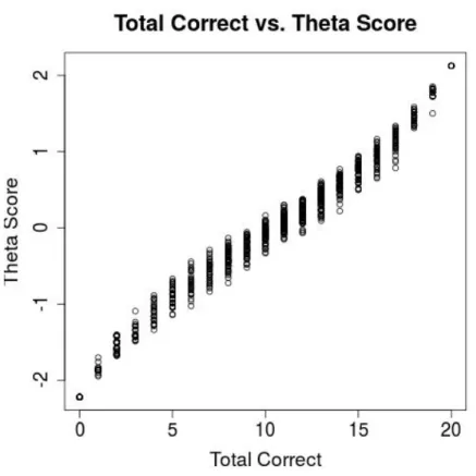
example. . . 38 2.4 ICCs for retained (solid) and removed (dotted) examples. . . 39 2.5 Plot of total correct answers vs. IRT scores. . . 40 3.1 Contour plots showing log-odds of labeling an example correctly for

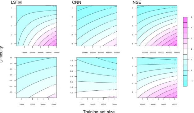
NLI (top row) and SA (bottom row) as a function of training set size (x-axis) and example difficulty (y-axis). Each line in the plots represents a single log-odds value for labeling an example correctly. Blue indicates low log-odds of labeling an example correctly, and pink indicates high log-odds of labeling an example correctly. The contour colors are consistent across plots and log-odds values are

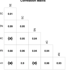
shown in the legend on the right. . . 52 3.2 Correlation matrix for theta scores and SNLI test set accuracy.

Correlations that are not significant (p <0.05) are crossed out. . . 55 4.1 Relative frequency histograms for the crowd-estimated probability of

(21)

4.2 Average KL-Divergence between sub-sampled crowd distributions and the estimated soft label distribution from the entire crowd data. Sampling 20 crowd workers achieves a good estimate of the label distributions without the cost of using the full 1000 worker

population. . . 77 5.1 Comparison of learned example difficulty parameters for human

(x-axis) and machine data (y-axis) for NLI (Fig. 5.1a) and SA (Fig. 5.1b). Spearman ρ (NLI): 0.409 (LSTM) and 0.496 (NSE).

Spearmanρ (SA): 0.332 (LSTM) and 0.392 (NSE). . . 88 5.2 Test set accuracy by filtering strategy for NLI (left) and SA (right)

plotted against percentage of training data retained. In both tasks filtering using the AVI strategy is most efficient in terms of high

accuracy for small training set sizes. . . 90 5.3 Test set accuracy for MNIST and CIFAR for each filtering strategy

plotted as a function of the percentage of training data retained. . . 91 5.4 Density plot of learned difficulties for SNLI and SSTB (left) and

MNIST and CIFAR (right) data sets. . . 93 5.5 The easiest (first and third rows) and hardest (second and fourth rows)

examples in the MNIST and CIFAR test sets. . . 96 6.1 (6.1a) A typical curriculum learning framework, where examples are

added at each epoch according to a static monotonically-increasing learning schedule. (6.1b) DDaCLAE estimates ability at each training epoch to dynamically select appropriate training data

given the model’s current ability. . . 105 6.2 Test set accuracy as a function of training epoch for each data set

tested. Vertical lines indicate the point at which each method had the highest dev set accuracy (for early stopping). Dotted lines indicate the percentage of training data used by each method at a given epoch. For MNIST, CIFAR, and SSTB, models trained with DDaCLAE converge more quickly than all other training setups. For SNLI, the baseline (training with all data) outperforms all curriculum learning setups. Note: the y-axis has been truncated for each plot to improve visibility. Figure best viewed in color. . . 110 7.1 Visualization of the question generation and validation process for the

(22)

7.2 Box plots of Turker scores on the AMT per-topic and validation tasks. Average raw score is above 70% in all cases. Counts indicate the

number of AMT responses retained after quality-control. . . 127 7.3 Results of analysis to identify useful items from the question sets.

Items were removed according to the reasons outlined in the

Methodology. . . 130 7.4 Test information curve for the full ComprehENotes instrument (55

items) and various subsets. . . 131 7.5 Flowchart describing our experiment. Amazon Mechanical Turk

workers were randomly assigned to one of three tasks on the platform. They completed the ComprehENotes test with the use of the provided external tool. All scores were then collected, and ability estimated were obtained using Item Response Theory

(IRT). . . 138 7.6 Example showing NoteAid simplified text. . . 139 7.7 Box plot of raw scores for baseline and treatment Turker groups. The

treatment groups were able to use MedlinePlus and NoteAid,

respectively, when taking the ComprehENotes test. . . 143 7.8 Box plot of ability estimates for baseline and treatment Turker groups.

The treatment groups MLP and NA were able to use MedlinePlus and NoteAid, respectively, when taking the ComprehENotes test.

(23)

INTRODUCTION

A typical supervised learning setup in machine learning involves using a large annotated training data set to fit a model capable of learning patterns in the training data in such a way that the model can generalize to an unseen test data set. Learning involves updating the model parameters according to differences between the model output and a single true, gold-standard label. The input data, which interacts with the model weights to provide the model output, is often taken as given. The output also is relatively static when compared to the work on model tuning. The gold-standard is the gold-standard, and we want our model to fit well to the data while also being able to generalize well. These gold-standard examples are fixed, and specific characteristics of the examples do not affect evaluation.

Once trained, model performance is evaluated by labeling a previously unseen data set and comparing the output labels to the known, gold-standard labels for that data set. Accuracy, recall, precision and F1 scores are commonly used to evaluate NLP applications. These metrics assume that each point in the data set has equal weight for evaluating performance. However examples are different. Some may be so hard that most/all NLP systems answer incorrectly; others may be so easy that every NLP system answers correctly. Neither example type provides meaningful information about the performance of an NLP system. Examples that are answered incorrectly by some systems and correctly by others are useful for differentiating systems according to their individual characteristics.

We propose an integration of psychometrics and machine learning to better model the supervised learning task. This integration allows for the modeling of input data latent traits as well as model latent traits to both inform the model-training procedure

(24)

and provide more insight into model generalization performance. The psychometric methodologies used here are known as Item Response Theory (IRT) [Baker, 2001,Baker and Kim, 2004].

IRT is one of the most widely used methodologies in psychometrics for scale con-struction and evaluation. It is typically used to analyze human responses (graded as right or wrong) to a set of questions (called “items” in the psychometric literature and examples here). With IRT, individual ability and example characteristics are jointly modeled to predict performance [Baker and Kim, 2004]. This statistical model assumes the following: (a) Individuals differ from each other on an unobserved latent trait dimension (called “ability” or “factor”); (b) The probability of correctly answering an example is a function of the person’s ability and of the example’s latent parameters. This function is called item characteristic curve (ICC) and involves example charac-teristics as parameters; (c) Responses to different examples are independent of each other for a given ability level of the person (“local independence assumption”); (d) Responses from different individuals are independent of each other.

First, we introduce two new test sets for natural language inference and sentiment analysis built using IRT that measure the latent ability of a natural language processing model as opposed to raw accuracy, and show that these tests provide more insight into model performance than traditional evaluation such as accuracy or F1. By using IRT, the latent characteristics of specific test set examples affect a model’s score. At the same time, the latent ability parameter of a model places the model on a continuum of ability with other test-takers, which allows for comparison between models more informative than a simple accuracy score. With IRT, we show that high accuracy is not necessarily indicative of high performance if a test data set is very easy.

Second, we show that by modeling the difficulty of test set examples, patterns emerge when training deep neural network models that are consistent with human learning patterns, specifically, that as models are trained with larger training sets,

(25)

they learn easy test set examples more quickly than hard items. We find that there is a relationship between example difficulty and model performance, not only for fully trained models but also as a function of the training set size used to train the model. This allows for new insights into how models behave under different training circumstances, and quantitatively confirms insights about learning that have been used in methods such as curriculum learning.

Third, we propose a soft-label memorization-generalization training sequence for deep neural networks that leverages human uncertainty about data to fine-tune deep learning models. Soft labels for a small sample of data points are estimated by calculating the distribution over potential labels gathered from Amazon Mechanical Turk workers. By fine-tuning three representative deep learning architectures with soft labels we are able to improve test set performance.

Fourth, we propose a new method for modeling latent example and model charac-teristics using IRT at a large scale. At present there has not been work done to build very large scale IRT models because the models are typically used to evaluate humans. We use variational inference methods to estimate the latent parameters that allow for much larger scale modeling of the data than previously done.

Fifth, we propose a dynamic data selection strategy for curriculum learning that estimates model competency during training in order to select training data examples that are most appropriate for a learner at a point in time. This allows for selecting training examples based on model competency and not a rigid learning schedule. Dynamic data selection leads to more efficient and effective models.

Finally, we introduce a new test for measuring human Electronic Health Record (EHR) note comprehension and conduct experiments that demonstrate the ability of active educational interventions to improve note comprehension in patients. In the past patient understanding of their EHR notes has only been measured by self-reported patient data. We have developed a test using IRT to evaluate patient latent ability

(26)

for EHR note comprehension. This test is the first of its kind, and all questions in the test were automatically identified and extracted from de-identified patient EHR notes. The test demonstrates a real-world use case for the IRT test construction methods in the important area of patient health literacy, specifically with regards to EHRs and EHR notes.

In this dissertation we introduce new methods for test set construction and model evaluation for the machine learning and natural language processing community. In addition, we introduce a new way to learn IRT latent parameters for data sets at machine learning scale that tightly integrates input data information and parameter updating for improved generalization. We demonstrate that the integration of psy-chometrics into machine learning model training allows for more information about a data set to be used when training a model, leading to more efficient and effective learning. Finally, we present a new test for patient health literacy that will hopefully contribute to future research on measuring and improving patient health literacy. It is our hope that the methods proposed here provide researchers with new methods for training and evaluating models that do more than just use data but take properties of the data and models into account.

(27)

CHAPTER 1 BACKGROUND, FOUNDATIONS, AND NOTATION

Our goal is to bring psychometrics to machine learning by demonstrating the usefulness of psychometric methods, specifically Item Response Theory (IRT), on machine learning model training and evaluation. In this chapter we will provide an introduction to IRT for machine learning researchers, and an overview of the machine learning models and training methods that will be used to demonstrate the effectiveness of IRT for the benefit of psychometricians.

In typical machine learning evaluation, aggregate scores such as accuracy are calculated on a held-out test set. The characteristics of individual test set examples such as difficulty are not taken into consideration. Often times, the difficulty of a data set is determined after the fact, once it has been shown that certain baseline models do not do particularly well on the task. There is a need to model the intrinsic difficulty of the data sets used in machine learning to help guide progress in the field and to help place the progress of new models into context. For example, if a new machine learning model outperforms the state-of-the-art for a particular task by 0.01%, what does that really tell us about the new model? It could be that this new model labeled all but 3 test examples the exact same way as the previous state-of-the-art model. But for those 3, if the new model labels the easiest one incorrectly and the two harder examples correctly, while the prior model labeled the easiest example correctly but labeled the the two harder examples incorrectly, what does that mean in terms of which model should be used moving forward? Or, what does that tell us about the data set in question? Even if the new model achieves state-of-the-art performance, is

(28)

it acceptable that the model labels the easiest example incorrectly? In order to even know which example is the easiest, there needs to be a way to estimate the difficulty of each example.

Psychometrics is a field in psychology concerned with the evaluation of humans and the design of tests to evaluate those humans. IRT models are psychometric models that estimate the latent ability of humans in certain areas based on their responses to a carefully selected set of examples. These examples also have latent parameters such as difficulty that are learned by gathering a large number of response patterns from individuals. To date, there has been very little work on applying IRT methods in the machine learning community. We propose applying IRT methods to model latent characteristics of supervised learning models and of the data used to train and evaluate them. Specifically, we propose and evaluate the following thesis:

Estimating the characteristics of individual data points such as difficulty and latent model ability using psychometric methods can be done at a large scale, can improve model performance, and can allow for more thorough model evaluation.

1.1 Foundations

The methods described in this thesis apply to supervised machine learning models. For consistency we now define terms that will be used in the subsequent chapters. When there is inconsistency between the IRT and machine learning terminology it will be explicitly mentioned below, and the machine learning terminology will be used moving forward.

Definition 1.1.1 (Example). An example d is a tupled= (x, y), where x is a set of features associated with the example, andy is the gold-standard label for the example. Each y comes from a set of labels Y∗ ={y0, y1, . . . , yn−1}, where n is the number of possible class labels for the task. Y∗ is task-specific. For example, for the task of

(29)

sentiment analysis n = 2 and Y∗ ={positive, negative}. Examples are referred to as

items in the IRT literature.

Definition 1.1.2(Data set). A data set is a collection of examplesD={d0, d1, . . . , dn−1}, wheren is the number of examples in the data set. XD _{is the set of features associated}

with the examples in D, where XD

0 refers to the features of the first example in D.

YD is the set of gold-standard labels associated with the examples in D, where Y₀D

refers to the gold-standard label of the first example inD. Data sets may be used for model training or evaluation. Data sets used for training are training sets. Data sets used for evaluation are test sets (typically referred to as evaluation scales in the IRT literature).

Definition 1.1.3 (Model). A model provides label predictions for a test set. More formally, for some test setDtest, a modelM generates label predictions ˆYDtest based

on the features of Dtest, XDtest: ˆYDtest = M(XDtest), which are compared to the

gold-standard labels YDtest. A model is analogous to a subject in the IRT literature. In this work model will refer to a machine learning model, and if humans are involved they will be referred to as subjects.

Definition 1.1.4 (Response Pattern). A response pattern is a binary vector that compares a model’s label predictions for a test set with the gold-standard labels. For any model M and data set D,M’s response pattern is defined as:

ZM,D = [_I[ˆy0 =y0], . . . ,I[ˆyn =yn]] (1.1)

where _I[A] is the indicator function, which evaluates to 1 when the expression A is true and 0 when the expression is false.

(30)

1.2 Supervised Learning Evaluation

The goal of this thesis is to demonstrate the usefulness of psychometric methods, specifically IRT, for training and evaluating supervised machine learning models. In a typical supervised learning setup, a model is trained on some labeled data set which consists of features and labels. Each example is defined by the features associated with it and each example has a corresponding gold-standard label.

Current gold-standard data set generation methods include web crawling [Guo et al., 2013], automatic and semi-automatic generation [An et al., 2003], and expert [Roller and Stevenson, 2015] and non-expert human annotation [Bowman et al., 2015, Wiebe et al., 1999]. In each case validation is required to ensure that the data collected is appropriate and usable for the required task. Automatically generated data can be refined with visual inspection or post-collection processing. Human annotated data usually involves more than one annotator, so that comparison metrics such as Cohen’s or Fleiss’κ can be used to determine how much they agree. Disagreements between annotators are resolved by researcher intervention or by majority vote.

Evaluating these models requires a set of labeled data that was previously unseen by the model, to determine how well the model can generalize outside of the data the model was trained on. This held out test set is typically drawn from the same distribution as the training data. Model evaluation therefore consists of having the trained model generate labels for the test set and comparing these with the gold-standard labels.

There are many methods for how the test sets are obtained. For large data sets, there is typically a pre-defined held out test set to facilitate direct comparison between models. For smaller data sets, methods such as cross-validation are used, where the full data set is split into folds, and copies of the models are trained on all folds but one, which is held out for testing. Evaluation statistics across models are aggregated. We focus on model evaluation via a standard, held-out test set. This is the norm for

(31)

evaluating deep learning models on large benchmark data sets, as they are typically released with a pre-defined test set for model comparisons.

To evaluate model training, one typically considers accuracy on the training set. Continual improvement in training set accuracy indicates that the model is “learning” by being better able to classify the instances to which it has been exposed. Most common in machine learning experiments is the arithmetic mean:

Definition 1.2.1 (Training error). The training error of a model M refers to the percentage of examples in a training setDtrain that the model labels incorrectly:

etrain = 1− 1 N N X n=1 zMi,Dtrain (1.2)

Once a model has been trained, generalization performance is measured by the arithmetic mean on the held-out test set.

Definition 1.2.2 (Test error). The test error of a model M refers to the percentage of examples in a test setDtest that the model labels incorrectly:

etest = 1− 1 N N X n=1 zMi,Dtest (1.3)

Other performance metrics exist but are less common in the ML literature. For example, the geometric mean uses the product of responses instead of the sum. This more strictly penalizes incorrect answers.

Definition 1.2.3 (Geometric mean). For some response pattern Z the geometric mean is: ( N Y i=1 zM_i )N1 (1.4)

(32)

1.3 Item Response Theory

IRT is a methodology of evaluation for characterizing test examples and estimating subject ability from their performance on such tests. IRT assumes that individual test questions (referred to as “items” in IRT and “examples” here) have unique characteristics such as difficulty and discriminating power. These characteristics can be identified by fitting a joint model of human ability and examples characteristics to human response patterns to the test examples. Examples that do not fit the model can be removed and the remaining examples can be considered a scale to evaluate performance. IRT assumes that the probability of a correct answer is associated with both example characteristics and individual ability, and therefore a collection of examples of varying characteristics can determine an individual’s ability overall.

IRT accounts for differences among examples when estimating a subject’s ability. In addition, ability estimates from IRT are on the ability scale of the population used to estimate example parameters. For example, an estimated ability of 1.2 can be interpreted as 1.2 standard deviations above the average ability in this population. The traditional total number of correct responses generally does not have such quantitative meaning.

IRT has been widely used in educational testing. For example, it plays an instru-mental role in the construction, evaluation or scoring of standardized tests such as Test of English as a Foreign Language (TOEFL), Graduate Record Examinations (GRE) and SAT.

1.3.1 IRT Models

The simplest IRT model assumes a single latent parameter for each example, bi,

corresponding to the example’s difficulty, as well as a latent ability parameter for each model, θj. This is known as the one parameter logistic (1PL) model or the Rasch

(33)

The probability that model (or subject) j will answer example i correctly is:

p(yij = 1|θj, bi) =

1

1 +e−(θj−bi) (1.5)

The probability that model j will answer example iincorrectly is:

p(yij = 0|θj, bi) = 1−p(yij = 1|θj, bi) (1.6)

With a 1PL model, there is an intuitive relationship between difficulty and ability. An example’s difficulty value b can be thought of as the point on the ability scale where an individual (or model) has a 50% chance of answering correctly. Put another way, a model has a 50% chance of answering an example correctly when model ability is equal to example difficulty (if θj =bi in Equation 1.5).

Another common model is the three parameter logistic model (3PL):

pij(θj) = ci+

1−ci

1 +e−ai(θj−bi) (1.7)

where ai, bi, and ci are example parameters: the slope or discrimination parameter ai is related to the steepness of the curve, the difficulty parameter bi is the level of

ability that produces a chance of correct response equal to the average of the upper and lower asymptotes, and the guessing parameter ci is the lower asymptote of the

ICC and the probability of guessing correctly. A two-parameter logistic (2PL) IRT model assumes that the guessing parameters are 0.

1.3.2 Parameter Estimation

The likelihood of a data set of response patterns Z from multiple subjects to a set of examples given the parameters Θ and B is:

p(Z|Θ, B) = J Y j=1 I Y i=1 p(Zij =yij|θj, bi) (1.8)

(34)

−4 −2 0 2 4 0 0.2 0.4 0.6 0.8 1 θ p ( z = 1 | θ ,a, b, c )

Figure 1.1: Example ICC for a “good” example, fit as part of a 3PL Model. For this example, ai = 1, bi = 0, and ci = 0.25.

where zij = 1 if individual j answers example i correctly and zij = 0 if they do not.

The example parameters are typically estimated by marginal maximum likelihood (MML) via an Expectation-Maximization (EM) algorithm [Bock and Aitkin, 1981], in which subject parameters are considered random effectsθi ∼N(0, σ2θ) and marginalized

out. Once example parameters are learned, subjects’ θ parameters are scored typically with maximum a posteriori (MAP) estimation. IRT models are usually fitted to RPs of hundreds or thousands of human subjects, who usually answer at most 100 questions. Therefore the methods for fitting these models have not been scaled to huge data sets and large numbers of subjects (e.g. tens of thousands of machine learning models).

Figures 1.1 and 1.2 show examples of Item Characteristic Curves (ICCs) of two examples in a test set fit via a 3PL model. Figure 1.1 would be considered a “good” example, as there is a relatively steep slope distinguishing individuals that have a high probability of labeling the example correctly. Figure 1.2 would be considered a “bad” example. The slow increase in probability as ability increases indicates that this example is not useful for distinguishing between individuals. What’s more, the very large guessing parameter indicates that even individuals with low latent ability have

(35)

−4 −2 0 2 4 0 0.2 0.4 0.6 0.8 1 θ p ( z = 1 | θ ,a, b, c )

Figure 1.2: Example ICC for a “bad” example, fit as part of a 3PL Model. For this example, ai = 0.5, bi = 0, and ci = 0.4.

a high probability of labeling the example correctly. The ICC plots the probability of a model labeling an example correctly as a function of latent ability. A good example should exhibit an ICC relatively steep slope increasing between ability levels −3 and 3, where most people are located, in order to have appropriate power to differentiate different levels of ability.

1.3.3 IRT with Variational Inference

Variation inference (VI) is a model fitting method that approximates an intractable posterior distribution in Bayesian inference by a simpler variational distribution. Prior work has compared VI methods with traditional IRT methods [Natesan et al., 2016] and found it effective, but was primarily concerned with fitting IRT models for human-scale data.

Bayesian methods in IRT assume that the individual θ and b parameters in Eq. (2) both follow Gaussian prior distributions and make inference through the resultant joint posterior distribution π(θ, b|Y). As this posterior is usually intractable, VI approximates it by the variational distribution:

(36)

q(θ, b) = J Y j=1 πθ_j(θj) I Y i=1 πb_i(bi) (1.9)

Where π_jθ() andπ_ib() denotes different Gaussian densities for different parameters whose means and variances are determined by minimizing the KL-Divergence between

q(θ, b) and π(θ, b|Y).

The choice of priors in Bayesian IRT can vary. Prior work has shown that vague and hierarchical priors are both effective [Natesan et al., 2016]. We experiment with both in this work. A vague prior assumes θj ∼ N(0,1) and bi ∼ N(0,103), where

the large variance indicates a lack of information on the difficulty parameters. A hierarchical Bayesian model assumes

θj | mθ, uθ ∼N(mθ, u−θ1) bi |mb, ub ∼N(mb, u−_b1)

mθ, mb ∼N(0,106) uθ, ub ∼Γ(1,1)

Our results for these two options were very similar, so we only report those for hierarchical priors.

1.3.4 Building IRT Test Sets

To identify the number of factors in an IRT model, the polychoric correlation matrix of the examples is calculated and its ordered eigenvalues are plotted. The number of factors is suggested by the number of large eigenvalues. It can be further established by fitting (see below) and comparing IRT models with different numbers of factors. Such comparison may use model selection indices such as AIC and CBIC and should also take into account the interpretablility of the loading pattern that links examples to factors.

(37)

An IRT model can be fit to data by marginal maximum likelihood method through an EM algorithm [Bock and Aitkin, 1981]. The marginal likelihood function is the probability to observe the current observed response patterns as a function of the example parameters with the persons’ ability parameters integrated out as random effects. This function is maximized to produce estimates of the example parameters. For IRT models with more than one factor, the slope parameters (i.e. loadings) that relate examples and factors must be properly rotated [Browne, 2001] before they can be interpreted. Given the estimated example parameters, Bayesian estimates of the individual person’s ability parameters are obtained with the standard normal prior distribution.

After determining the number of factors and fitting the model, the local inde-pendence assumption can be checked using the residuals of marginal responses of example pairs [Chen and Thissen, 1997] and the fit of the ICC for each example can be checked with item fit statistics [Orlando and Thissen, 2000]. If both tests are passed and all examples have proper discrimination power, then the set of examples is considered a calibrated measurement scale and the estimated example parameters can be further used to estimate an individual person’s ability level.

1.3.5 Exploratory Model Fitting

Once a set of response patterns is gathered, it is not enough to simply fit an IRT model and use the result as your IRT test set. The first step is to identify a subset of examples that meet the underlying assumptions of IRT:

1. People differ from each other on an unobserved latent dimension of interest (usually called “ability”)

2. The probability of correctly answering a particular example is a function of the latent ability dimension (the item characteristic curve, ICC)

(38)

3. Responses to individual examples are independent of each other for a given ability level of a person (the “local independence assumption”)

4. Responses from different individuals are independent of each other.

In this section we describe the process of fitting an exploratory model. A number of software programs exist to automate portions of this process, in particular the mirt R package.

The first step is to confirm that there is a single underlying factor in the response pattern data set. If there are multiple latent factors, then a multi-factor model must be used, or the data must be split according to the latent factors to create multiple tests. To check the latent factors, you can plot the tetrachoric matrix to visualize the eigenvalues of the response pattern data. If there is a single large latent factor then you can proceed with a single factor model. This first step is crucial as it underlies the rest of the reasoning for building an IRT model. The goal is to develop a test that measures a latent ability parameter of some set of individuals for some task. If there are multiple latent factors in the data, then trying to learn a single latent θ will not accurately capture the data.

Once a single factor model has been confirmed as appropriate, the next step is to determine the most appropriate model given the characteristics of the examples. Is a 3 parameter logistic (3PL) model more appropriate than a 2 parameter logistic (2PL) model? That is, do we need to account for the guessing parameters for the examples in the data set? To do this one must first fit both 3PL and 2PL models (Chapter 2) and compare the model fits using traditional model fit statistics such as Akaike information criterion (AIC) [Akaike, 1974] or Bayesian Information Criterion (BIC) [Schwarz et al., 1978]. If a 2PL model is a better fit, than you can continue and not worry about the example guessing parameters. If the 3PL model is a better fit, the next step is to determine if, for each example in the response pattern set, the guessing parameter is significantly different from 0. For each example, if the guessing

(39)

parameter is not significantly different than 0 then a 2PL model is used. Therefore it is possible to construct a test model that is a combination of 2PL and 3PL models for each of the examples.

To identify the number of latent factors, a plot of eigenvalues of the tetrachoric correlation matrix can be inspected and a comparison between IRT models with different number of factors can be conducted. A target rotation [Browne, 2001] can be used to identify a meaningful loading pattern that associates factors and examples. If there are multiple latent factors present, the target rotation can be used to align the factors with specific sub-tasks. For example, in the case of NLI, if three latent factors are present, each factor can be interpreted as the ability of a user to recognize the correct relationship between the sentence pairs associated with that factor (e.g. contradiction).

1.3.6 Confirmatory Model Fitting

Once a model has been fit that best represents the response pattern data, it is important to confirm that the model did not overfit the data by conducting a confirmatory analysis. To do this, a new set of response patterns for the same set of examples are collected from a new population of test-takers. With the pre-fit example parameters, a new IRT model is fit to estimate θ and the model fit statistics are examined. If the fit statistics are reasonable, then the model is determined to be appropriate for the task. Otherwise, a new model must be fit.

1.3.7 Scoring

Estimating the ability of a model at a point in time is done with a “scoring” function. When example difficulties are known, model ability is estimated by maximizing the likelihood of the data given the response patterns and the example difficulties to obtain the ability estimate. All that is required is a single forward pass of the model on the data, as is typically done with a test or validation set.

(40)

Zj =∀y∈YI[yi = ˆyi] (1.10) L(θj|Zj) =p(Zj|θj) (1.11) ˆ θj = arg max θj I Y i=1 p(zij =yij|θj) (1.12)

1.4 Related Work

1.4.1 Uncertainty in Machine Learning

There are several other areas of study regarding how best to use training data that are related to this work. Re-weighting or re-ordering training examples is a well-studied and related area of supervised learning. Often examples are re-weighted according to some notion of difficulty, or model uncertainty [Bengio et al., 2009, Chang et al., 2017]. In particular, the internal uncertainty of the model is used as the basis for selecting how training examples are weighted. For example, the history of model predictions for an example up to time t−1 can be used to estimate the model probability of labeling the example correctly [Chang et al., 2017]. However, model uncertainty is dependent upon the original data set the model was trained on, and is representative of uncertainty with respect to this particular model. This can be considered a local measure of uncertainty and may not be comparable across models.

This work is related to transfer learning and domain adaptation [Caruana, 1995, Bengio et al., 2011,Bengio, 2012], but with an important distinction. Transfer learning and domain adaptation repurpose representations learned for a source domain to facilitate learning in a target domain. We want to improve performance in the source domain by fine-tuning with data from the source domain with distributions over class labels. This work differs from domain adaptation and transfer learning in that we are not adding data from a different domain or applying a learned model to a new task. Instead, we are augmenting a single classification task by using a richer representation

(41)

of where the data lies within the class labels to inform training. The goal is that by fine tuning with a distribution over labels, a model will be less likely to overfit on a training set.

Prior work has considered IRT in the context of evaluating ML models using machine-generated [Martınez-Plumed et al., 2016] response patterns. In one study the authors attempted to fit IRT models using machine generated response patterns on small data sets (i.e. 200-300 examples), but obtained results that are difficult to interpret using the existing IRT assumptions [Martınez-Plumed et al., 2016]. To the best of our knowledge no one has attempted to fit IRT models using DNN-generated response patterns on large data sets.

1.4.2 Latent Modeling for Crowds

Prior work has considered modeling latent characteristics of examples and/or models. In particular, latent-variable models have been developed to identify low-quality annotators (spammers) [Hovy et al., 2013]. The proposed model assumes that an annotator either produces the correct label or guess randomly with a guessing parameter varying only across annotators. Other work used the Dawid & Skene model in which an annotator’s response depends on both the true label and the annotator [Dawid and Skene, 1979, Passonneau and Carpenter, 2014]. In both models an annotator’s response depends on an example only through its correct label. In contrast, IRT assumes a more sophisticated response mechanism involving both annotator qualities and example characteristics. To our knowledge we are the first to introduce IRT to NLP and to create a gold standard with the intention of comparing NLP applications to human intelligence.

The quality of crowdsourced data for linguistics research has been evaluated as well [Munro et al., 2010]. In that work the authors recreate classic linguistic studies and provide evaluation metrics for the obtained data. They compare crowd-generated

(42)

data with controlled experiments, whereas we use the crowd to identify data set examples for a discriminating test set for future evaluations. Identifying true labels via latent-trait models in the past has relied on a small number of annotators [Bruce and Wiebe, 1999]. That work uses 4 annotators at varying levels of expertise and does not consider the discriminating power of data set examples.

1.4.3 Soft Labels

Other work on modeling uncertainty in labels is Knowledge Distillation [Hinton et al., 2015]. In Knowledge Distillation, output probabilities of a complex expert model are used as input to a simpler model so the simpler model can learn to generalize based on the output weights of the expert model. The expectation is that how an expert model assigns output weights can be used to reduce overfitting in the simpler model. However with Knowledge Distillation, the expert model that is distilling its knowledge was still trained with a single class label as the gold standard, and the expert passes its uncertainty to the simpler model. In our work we capture uncertainty at the original training data, in order to induce generalization as part of the original training.

This work is also related to the idea of “crowd truth” and the CrowdTruth platform for collecting and using annotations from the crowd [Kajino et al., 2012, Inel et al., 2014]. The crowd truth assumption is that disagreement between annotators provides signal about data ambiguity and should be used in the learning process. CrowdTruth includes several metrics to calculate likelihoods of different events with regards to particular examples and particular annotators. In those cases, particularly with regards to annotators, the metrics are used to identify potential low-quality annotators for removal. We have a large number of annotations for each example (1000 annotations per example), and therefore we assume that any issues of annotator quality will be “drowned out” by the large number of annotations. Therefore we do not need to

(43)

identify and remove annotations, and instead can use raw annotation metrics instead of the CrowdTruth metrics. In addition this work is closely related to the idea of Label Distribution Learning (LDL) from Computer Vision (CV) [Geng, 2016]. For training and testing, LDL assumes that y is a probability distribution over labels. With LDL, the goal is to learn a distribution over labels. However in our case we would still like to learn a classifier that outputs a single class, while using the distribution over training labels as a measure of uncertainty in the data. We use the distribution over labels to represent the uncertainty associated with different examples in order to improve model training.

To the best of our knowledge this is the first work to use a subset of soft labeled data for fine-tuning, whereas previous work used an all-or-none approach (all hard or soft labels).

1.4.4 One-Shot Learning

One area of ML research in a similar category to the IRT work proposed here is one-shot learning. One-one-shot learning is an attempt to build ML models that can generalize after being trained on one or a few examples of a class as opposed to a large training set [Lake et al., 2013]. One-shot learning attempts to mimic humanlearning behaviors

(i.e., generalization after being exposed to a small number of training examples) [Lake et al., 2013]. Our work instead looks at comparisons to human performance, where any learning (on the part of models) has been completed beforehand. Our goal is to analyze DNN models and training set variations as they affect ability in the context of IRT.

1.4.5 Curriculum Learning

Curriculum learning (CL) is a training procedure where models are trained to learn simple concepts before more complex concepts are introduced [Bengio et al., 2009]. CL training for neural networks can improve generalization and speed up convergence. In

(44)

curriculum learning the difficulty of examples is typically assigned based on heuristics of the data (e.g. the number of sides of a shape). IRT models directly estimate difficulty from the responses of human or machine test-takers themselves instead of relying on heuristics. Self-paced learning and the Leitner method use model performance to estimate difficulties, but are restricted to a single model’s performance, not a more global notion of difficulty [Kumar et al., 2010, Amiri et al., 2018].

Since its original proposal, curriculum learning has become a well-studied area of machine learning [Bengio et al., 2009]. The primary focus has been on developing new heuristics to identify easy and difficult examples in order to build a curriculum. Originally, curriculum learning methods were evaluated on toy data sets with heuristic measures of difficulty [Bengio et al., 2009]. For example, on a shapes data set, shapes with more sides were considered more difficult than shapes with fewer sides. Similarly, sentences with more words were considered more difficult than sentences with fewer words.

Recent work has shown that spaced repetition strategies (SR) can be effective for improving model performance [Amiri et al., 2017, Amiri, 2019]. Instead of using a traditional curriculum learning setup, spaced repetition bins examples based on estimated difficulty. The bins are shown to the model at differing intervals so that more difficult examples are seen more frequently than easier examples. This method has been shown to be effective for human learning, and results demonstrate effectiveness on NLP tasks as well. Similarly to traditional curriculum learning frameworks, SR uses model-dependent heuristics for difficulty and rigid schedulers to determine when training examples should be re-introduced to the learner.

Recent work has shown that measuring model competency during training to determine which examples to include at a training epoch further improves performance by matching data to model competency [Platanios et al., 2019]. However, in that work the model of competency is based on a heuristic rate of knowledge acquisition, and

(45)

does not actually measure model competency. To the best of our knowledge this is the first work to match model ability at a point in training with appropriate training data in a curriculum learning framework.

There has been recent work investigating the theory behind curriculum learning [Weinshall et al., 2018, Hacohen and Weinshall, 2019], particularly around trying to define an ideal curriculum. The authors explicitly identify the two key aspects of curriculum learning, namely “sorting by difficulty” and “pacing.” curriculum learning theoretically leads to a steeper optimization landscape (i.e. faster learning) while keeping the same global minimum of the task without curriculum learning. In that work there is still a reliance on “pacing functions” as opposed to an actual assessment of model ability at a point in time.

Hacohen and Weinshall also demonstrated a key distinction between curriculum learning and similar methods such as self-paced learning [Kumar et al., 2010], hard example mining [Shrivastava et al., 2016], and boosting [Freund and Schapire, 1997]: namely that the former considers difficulty with respect to the final hypothesis space (i.e. a model trained on the full data set) while the later methods consider ranking examples according to how difficult the current model determines them to be [Hacohen and Weinshall, 2019]. In this work we bridge the gap between these methods by probing model ability at the current point in training and using this estimated ability to identify appropriate training examples in terms of global difficulty.

(46)

CHAPTER 2 BUILDING NLP TEST SETS WITH ITEM RESPONSE

THEORY

In this chapter we will demonstrate the usefulness of using Item Response Theory (IRT) for building test sets. IRT has been used to build test sets for many years and in many contexts, and the methodology is well-established. Here, we apply these methods to natural language processing for the first time with two representative tasks: natural language inference (NLI) and sentiment analysis (SA).

The rest of this chapter is structured as follows: we first describe IRT and the process of building a test set with IRT in detail. Then, we describes the data collection, model fitting, and evaluation of the IRT NLP test sets. We then demonstrate the use of the test sets on deep learning models for each NLP task.

2.1 Item Response Theory for Test Set Generation

The process of building an IRT test set can be broken down into three parts: response pattern collection, exploratory model fitting, and confirmatory model fitting. We will describe each of these steps generally here, with specifics in the followings sections for the NLP and EHR comprehension tests, respectively. To begin one must first have a pool of examples from which the test set will be obtained. This could be a large pool of previously written questions, or a data set for a specific task in the context of NLP. For this example pool, a large IRT model is fit and examples are removed that do not fit, until you are left with a subset of examples that can estimate the latent dimension well.

(47)

Throughout this chapter the IRT model under consideration is the three parameter logistic (3PL) model, which was introduced in Section 1.3. Recall that the 3PL model estimates the probability that modelj will answer exampleicorrectly, given modelj’s latent abilityθj and examplei’s discriminatory parameterai, difficultybi, and guessing

parameter ci:

pij(θj) = ci+

1−ci

1 +e−ai(θj−bi) (2.1)

2.1.1 Gathering Response Patterns

Before building an IRT test set, there must first be some example pool from which a subset can be extracted as an IRT test. This pool of examples typically consists of questions that seem appropriate for measuring the desired trait, but have not yet been validated. For example, for the SAT there is a pool of examples that have been written as candidates for inclusion for the test. These examples are included in the test periodically and their latent characteristics are evaluated to determine if they should be included in the test [Carlson and von Davier, 2013].

To learn latent example parameters for a test set, one requires data. Specifically, it is necessary to first gather a large number of graded responses to the examples in the example pool in order to fit the IRT model. Following §1.1, let Dpool be the set

of examples in the example pool under consideration for inclusion, where XDpool _and YDpool _{are the features and gold-standard labels associated with the examples in the}

pool, respectively. For some set of modelsJ, let ˆyij be modelj’s labeling of example i.

Model j’s response pattern Zj is defined as the sequence of model j’s provided labels,

graded correct or incorrect against the gold standard label:

(48)

where _I[] is the indicator function, which evaluates to 1 when the expression is true and evaluates to 0 when the expression is false.

In a typical IRT testing scenario, response patterns are gathered from human subjects for a specific task. For example, new questions on the SAT are added to the test on a trial basis, and responses from students are gathered as they take the full test, and new questions are evaluated with respect to the existing test [Carlson and von Davier, 2013]. In other cases, a target population is identified and given the preliminary test questions, from which the IRT test set is identified. For example, a test of cancer patients was developed from response patterns taken from cancer patients [Mazor et al., 2012b, Mazor et al., 2012a]. However in our work, response patterns are gathered using crowdsourcing workers, specifically those on the Amazon Mechanical Turk (AMT) crowdsourcing platform.

AMT is an online microtask crowdsourcing platform where individuals (called Turkers) perform Human Intelligence Tasks (HITs) in exchange for payment. HITs are usually pieces of larger, more complex tasks that are have been broken up into multiple, smaller subtasks. AMT and other crowdsourcing platforms are used to build large corpora of human-labeled data at low cost compared to using expert annotators [Snow et al., 2008, Sabou et al., 2012]. Researchers’ projects have used AMT to complete a variety of tasks [Demartini et al., 2012, Zhai et al., 2013]. Recent research has shown that AMT and other crowdsourcing platforms can be used to generate corpora for clinical natural language processing and disease mention annotation [Zhai et al., 2013,Good et al., 2015]. AMT was used to detect errors in a medical ontology and found that the crowd was as effective as domain experts [Mortensen et al., 2015]. In addition, AMT workers have been used to identify disease mentions in PubMed abstracts [Good et al., 2015] and rank Adverse Drug Reactions in order of severity [Gottlieb et al., 2015] with good results.

(49)

In order to ensure that the data gathered from the AMT Turkers was reliable, we included a number of quality control mechanisms in each of our tests:

1. AMT task access was restricted to individuals located in the United States, as a proxy for requiring English speakers

2. Tasks were only available to Turkers who have a prior task approval rate of 97% or higher

3. Within each task periodic attention-check questions were included, designed to ensure that the Turkers were paying attention and answering the questions to the best of their ability. Responses where the attention-check questions were answered incorrectly were removed.

For each of our IRT tests, we gathered enough response patterns based on the size of our example banks to ensure that the fit IRT models were reliable. While there is no set standard for sample sizes in IRT models, this sample size satisfies the standards based on the non-centralχ2 _{distribution [MacCallum et al., 1996] used when} comparing two multidimensional IRT models. This sample size is also appropriate for tests of example fit and local dependence that are based on small contingency tables. To identify appropriate examples for the test sets we conducted both exploratory (§1.3.5) and confirmatory (§1.3.6) analysis of the response pattern data.

We built a unidimensional IRT model for each set of examples associated with a single factor. We fit and compared one- and two-factor 3PL models to confirm the unidimensional structure underlying these examples, assuming the possible presence of guessing in people’s responses. We further tested the guessing parameter of each example in the one factor 3PL model. If it was not significantly different from 0, a 2PL ICC was used for that particular example.

Once an appropriate model structure was determined, individual examples were evaluated for goodness of fit within the model. If an example was deemed to fit the