A BAYESIAN LOCAL CAUSAL DISCOVERY
FRAMEWORK
by
Subramani Mani
MBBS, Medical College Trivandrum, 1987
MS (Computer Science), University of South Carolina, 1994
Submitted to the Graduate Faculty of
the School of Arts and Sciences in partial fulfillment
of the requirements for the degree of
Doctor of Philosophy
University of Pittsburgh
2005
UNIVERSITY OF PITTSBURGH
SCHOOL OF ARTS AND SCIENCES
This dissertation was presented
by
Subramani Mani
It was defended on
May 17, 2005
and approved by
Gregory F. Cooper, Department of Medicine and the Intelligent Systems Studies Program,
University of Pittsburgh
Michael M. Wagner, Department of Medicine and the Intelligent Systems Studies Program,
University of Pittsburgh
Peter Spirtes, Department of Philosophy, Carnegie Mellon University
Bruce G. Buchanan, University Professor of Computer Science (Emeritus), Department of
Computer Science, University of Pittsburgh
Dissertation Director: Gregory F. Cooper, Department of Medicine and the Intelligent
Copyright c° by Subramani Mani 2005
A BAYESIAN LOCAL CAUSAL DISCOVERY FRAMEWORK
Subramani Mani, PhD
University of Pittsburgh, 2005
This work introduces the Bayesian local causal discovery framework, a method for discovering unconfounded causal relationships from observational data. It addresses the hypothesis that causal discovery using local search methods will outperform causal discovery algorithms that employ global search in the context of large datasets and limited computational resources. Several Bayesian local causal discovery (BLCD) algorithms are described and results pre-sented comparing them with two well-known global causal discovery algorithms PC and FCI, and a global Bayesian network learning algorithm, the optimal reinsertion (OR) algorithm which was post-processed to identify relationships that under assumptions are causal.
Methodologically, this research formalizes the task of causal discovery from observational data using a Bayesian approach and local search. It specifically investigates the so called Y structure in causal discovery and classifies the various types of Y structures present in the data generating networks. It identifies the Y structures in the Alarm, Hailfinder, Barley, Pathfinder and Munin networks and categorizes them. A proof of the convergence of the BLCD algorithm based on the identification of Y structures, is also provided. Principled methods of combining global and local causal discovery algorithms to improve upon the performance of the individual algorithms are discussed. In particular, a post-processing method for identifying plausible causal relationships from the output of global Bayesian network learning algorithms is described, thereby extending them to be causal discovery algorithms.
In an experimental evaluation, simulated data from synthetic causal Bayesian networks representing five different domains, as well as a real-world medical dataset, were used. Causal
discovery performance was measured using precision and recall. Sometimes the local methods performed better than the global methods, and sometimes they did not (both in terms of precision/recall and in terms of computation time). When all the datasets were considered in aggregate, the local methods (BLCD and BLCDpk) had higher precision. The general performance of the BLCD class of algorithms was comparable to the global search algorithms, implying that the local search algorithms will have good performance on very large datasets when the global methods fail to scale up. The limitations of this research and directions for future research are also discussed.
Keywords: Causality, Causal Bayesian networks, Causal discovery, Global search, Local search, Markov blanket, BLCD, Y structure, Infant mortality.
TABLE OF CONTENTS
PREFACE . . . xvii
1.0 WHY CAUSAL DISCOVERY? . . . 1
1.1 INTRODUCTION . . . 1
1.2 HYPOTHESIS FOR CAUSAL DISCOVERY . . . 3
2.0 BACKGROUND: FRAMEWORK FOR CAUSAL DISCOVERY. . . . 6
2.1 BAYESIAN NETWORKS . . . 6
2.2 CAUSAL BAYESIAN NETWORKS . . . 7
2.3 CAUSAL INFLUENCE, CONFOUNDED AND UNCONFOUNDED CAUSAL RELATIONSHIPS . . . 9
2.4 ASSUMPTIONS FOR CAUSAL DISCOVERY . . . 11
2.4.1 The causal Markov condition . . . 12
2.4.2 The causal faithfulness condition . . . 14
2.4.2.1 The problem of deterministic relationships. . . 15
2.4.2.2 Goal oriented systems . . . 16
2.5 BAYESIAN SCORING OF COMPLETE CAUSAL MODELS . . . 18
2.6 BAYESIAN MODEL AVERAGING (BMA) . . . 19
2.7 SELECTIVE BAYESIAN MODEL AVERAGING AND MODEL SELEC-TION . . . 19
2.8 HANDLING MISSING DATA . . . 20
3.0 RELATED WORK: LEARNING CAUSAL BAYESIAN NETWORKS FROM DATA . . . 22
3.1.1 PC algorithm . . . 23
3.1.2 FCI algorithm. . . 26
3.1.2.1 Population inference assumption (Spirtes et al., 1999) . . . 26
3.1.2.2 O-Equiv(Cond) (Spirtes et al., 1999) . . . 27
3.1.2.3 Partial ancestral graph (Spirtes et al., 1999). . . 27
3.1.2.4 FCI Pseudocode . . . 29
3.1.2.5 Anytime FCI (AFCI) . . . 30
3.1.3 GS Markov blanket algorithm . . . 31
3.2 BAYESIAN NETWORK EQUIVALENCE . . . 32
3.2.1 Independence equivalence . . . 32
3.2.2 Distribution equivalence . . . 33
3.2.3 Hypothesis equivalence . . . 33
3.2.4 Likelihood equivalence . . . 34
3.3 SCORE BASED LEARNING ALGORITHMS . . . 35
3.3.1 Hidden variables . . . 37
3.3.2 Instrumental variables . . . 38
3.4 LOCAL SEARCH BASED METHODS . . . 39
3.4.1 LCD . . . 39
3.4.2 Silverstein algorithm . . . 41
3.4.3 Instrumental variable (IV) algorithm . . . 42
3.5 MDL METHODS . . . 43
3.6 LEARNING AND REPRESENTING LOCAL PARAMETER STRUCTURE USING OTHER FORMALISMS . . . 46
3.7 HYBRID METHODS OF LEARNING NETWORKS . . . 47
4.0 PRIOR WORK . . . 52
4.1 LCD VARIANTS—ALGORITHM DESCRIPTION . . . 52
4.1.1 LCDa, LCDb and LCDc . . . 53
4.1.2 Contextual causal influences—LCDm . . . 54
4.2 LCD VARIANTS—RESULTS AND DISCUSSION . . . 55
5.1 The BAYESIAN LOCAL CAUSAL DISCOVERY (BLCD) FRAMEWORK
AND BLCD ALGORITHM . . . 65
5.1.1 Y structure . . . 69
5.1.2 Scoring the DAGs . . . 74
5.1.3 Scoring Measure . . . 75
5.1.4 BLCD steps . . . 76
5.1.5 Time complexity of BLCD . . . 78
5.1.6 Proof of correctness of BLCD . . . 78
5.1.7 Incorporating prior knowledge in BLCD . . . 79
5.2 EXTENSIONS TO BLCD . . . 85
5.2.1 BLCDvss: Making use of shielded colliders . . . 85
5.2.2 BLCDcv: CombiningX and Z variables . . . 87
6.0 EXPERIMENTAL METHODS . . . 89
6.1 Y STRUCTURES FROM PC, FCI AND OR . . . 90
6.2 SYNTHETIC BAYESIAN NETWORKS . . . 91
6.3 EXPERT DESIGNED CAUSAL NETWORKS . . . 92
6.3.1 Network evaluation . . . 92
6.3.2 The Alarm network. . . 97
6.3.3 The Hailfinder network. . . 97
6.3.4 The Barley network . . . 97
6.3.5 The Pathfinder network . . . 98
6.3.6 The MUNIN network. . . 98
6.3.7 Dataset generation . . . 98
6.3.8 Evaluation metrics for simulated causal network data . . . 99
6.4 REAL-WORLD DATABASES . . . 99
6.4.1 Infant Birth and Death Dataset . . . 99
6.4.2 Prior knowledge for real-world datasets . . . 103
6.5 EXPERIMENTAL RUNS . . . 103
7.0 RESULTS . . . 105
7.2 PC AND FCI RESULTS . . . 113
7.3 BLCD RESULTS . . . 114
7.3.1 Based on what is theoretically discoverable by the algorithm . . . . 114
7.3.2 Based on the union of discoverable causes across all algorithms . . 118
7.3.2.1 Precision-recall graphs for each dataset . . . 118
7.3.2.2 Summary tables for each algorithm. . . 124
7.3.2.3 A global summary table over all the simulated datasets . . 127
7.4 LCD RESULTS . . . 129
7.5 INFANT DATASET RESULTS . . . 131
7.6 RUNTIMES . . . 136 8.0 DISCUSSION . . . 137 8.1 ALARM . . . 140 8.2 HAILFINDER . . . 140 8.3 BARLEY . . . 140 8.4 PATHFINDER . . . 140 8.5 MUNIN . . . 141 8.6 INFANT . . . 143
8.7 IMPLICATIONS FOR CAUSAL DISCOVERY . . . 143
8.8 CONTRIBUTIONS . . . 147
8.9 LIMITATIONS . . . 147
8.9.1 Causal discovery framework limitations . . . 148
8.9.2 Specific algorithmic and experimental methodological limitations . 148 8.10 FUTURE WORK AND OPEN PROBLEMS . . . 149
APPENDIX A. ADDITIONAL RESULTS . . . 151
APPENDIX B. BLCD EQUATION . . . 157
APPENDIX C. Y STRUCTURE THEOREMS . . . 159
APPENDIX D. MARKOV BLANKET THEOREMS. . . 170
D.1 PROOF . . . 171
D.1.1 The components of the score. . . 171
D.1.3 Backward search . . . 172 BIBLIOGRAPHY . . . 173 INDEX . . . 180
LIST OF TABLES
1 LCDm statistical tests for the models shown in Figure 19 . . . 60
2 Conditional probability table of cirrhosis given alcoholic . . . 60
3 LCDm output—X causally influencing Y, and the number of multivariate in-fluences for X →Y . . . 61
4 Infant outcome given infant birth weight. . . 62
5 Infant outcome given infant birth weight and maternal disease . . . 64
6 DAG generation from a four node setF . . . 72
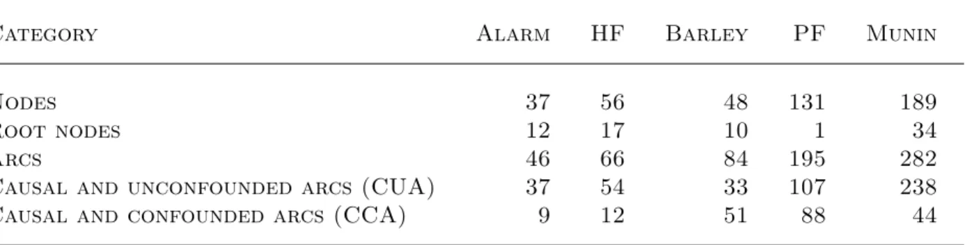
7 Categories of node pairs in the Alarm, Hailfinder, Barley, Pathfinder, and Munin networks . . . 93
8 Nodes and arcs in the Alarm, Hailfinder, Barley, Pathfinder, and Munin networks 94 9 A best case scenario output for PC, FCI, BLCD, and LCD algorithms for the causal Bayesian network shown in Figure 36. . . 95
10 Gold standard labels for Infant data . . . 101
11 Platinum standard labels for Infant data. . . 102
12 A synopsis of the LCD algorithms used . . . 106
13 A synopsis of BLCD, OR, PC and FCI . . . 107
14 Types of Y structures and algorithms that output them (see also Figures 38 and 39) . . . 110
15 Types of “Y” structures in the Alarm, Hailfinder, Barley, Pathfinder, and Munin networks . . . 111
16 OR precision and recall on different datasets based on global Y arcs (20,000 samples). . . 112
17 PC precision and recall on different datasets based on global Y arcs (20,000
samples). . . 113
18 BLCD precision and recall based on unshielded and unconfounded Y arcs (20,000 samples).. . . 114
19 BLCDpk precision and recall based on unshielded and unconfounded Y arcs (20,000 samples).. . . 115
20 BLCDvss precision and recall based on Mshielded and unshielded but uncon-founded Y arcs (20,000 samples). . . 116
21 BLCDcv precision and recall based on unshielded and unconfounded Y arcs (20,000 samples).. . . 117
22 BLCD precision and recall based on global Y arcs (20,000 samples). . . 124
23 BLCDpk precision and recall based on global Y arcs (20,000 samples). . . 125
24 BLCDvss precision and recall based on global Y arcs (20,000 samples). . . 125
25 BLCDcv precision and recall based on global Y arcs (20,000 samples). . . 126
26 Precision and recall based on global Y arcs from all datasets (20,000 samples). 127 27 Dataset aggregation: Precision significance based on all the 229 global Y struc-tures . . . 128
28 LCDa, LCDb, LCDc precision based on causal and unconfounded pairs (20,000 samples). . . 129
29 LCDa, LCDb, LCDc recall based on causal and unconfounded pairs (20,000 samples). . . 130
30 Infant: Summary results (20,000 samples). . . 131
31 Algorithm runtimes in seconds for the different datasets. . . 136
32 Alarm to Munin: Based on what is theoretically discoverable for each algorithm138 33 Alarm to Munin: Based on the union of what is discoverable over all the algorithms (global Y structures) . . . 138
34 Effect of combining PC and BLCD on Munin dataset (20,000 instances) . . . 145
35 Alarm: Precision based on global Y arcs with increasing sample sizes. . . 151
36 Alarm: Recall based on global Y arcs with increasing sample sizes. . . 152
38 Hailfinder: Recall based on global Y arcs with increasing sample sizes. . . 153
39 Barley: Precision based on global Y arcs with increasing sample sizes. . . 153
40 Barley: Recall based on global Y arcs with increasing sample sizes. . . 154
41 Pathfinder: Precision based on global Y arcs with increasing sample sizes. . . 155
42 Pathfinder: Recall based on global Y arcs with increasing sample sizes. . . 155
43 Munin: Precision based on global Y arcs with increasing sample sizes. . . 156
LIST OF FIGURES
1 A hypothetical causal Bayesian network structure . . . 8
2 Three hypothetical causal models in which S causes C. . . 11
3 A CBN with three nodesX1,X2, and X3. . . 13
4 A CBN with two nodesX1, and X3. . . 14
5 A CBN with three nodesX1,X2, and X3. . . 15
6 A CBN with three nodesX1,X2, and X3. . . 15
7 A CBN with three nodesX1,X2, and X3. . . 16
8 A CBN with three observed nodes—X1,X2, X3, and one hidden node H. . . 16
9 A hypothetical Bayesian network structure . . . 24
10 Two-variable independence-equivalent Bayesian networks . . . 32
11 Three-variable independence-equivalent Bayesian networks . . . 32
12 A “V” structure over variables X, Y, and Z. . . 32
13 Bayesian network structure X →Y →Z annotated with conditional indepen-dence relationships. . . 50
14 Causal models in which X causes Y; H denotes a hidden variable(s). . . 50
15 Causal model in which W causes X, and X and Y are dependent due to confounding by a hidden variable(s) represented byH. . . 51
16 Three causal models for variables W, X and Y . . . 51
17 A model that satisfies the CCU rule and is confounded . . . 51
18 Two causal models with equivalent independence relationships . . . 51
19 Selected causal models in whichW causesX, andXcausesY;M acts as a covariate ofY. H denotes a hidden variable(s). . . 59
20 A causally-confounded pattern output by LCDa, but not by LCDb or LCDc.
A double arrow denotes a path length greater than one. . . 60
21 Influence of Birth Weight on Infant Mortality . . . 62
22 Multivariate Influence on Infant Mortality . . . 63
23 A “V” structure—X is a collider in this Figure . . . 66
24 A “shielded” collider—X is a shielded collider in this example. . . 66
25 Several causal models that contain four nodes out of the possible 543 models. 67 26 Four causal models containing one or more hidden variables that represent the same independence relationships of the corresponding models shown in Figure 25. A hidden variable is represented with the letter H. . . 68
27 Four causal models out of the 543 that belong to the same equivalence class.. 72
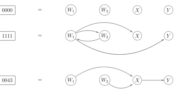
28 Three unconstrained directed graphs and their codes. The code 0043 represents the Y structure. . . 73
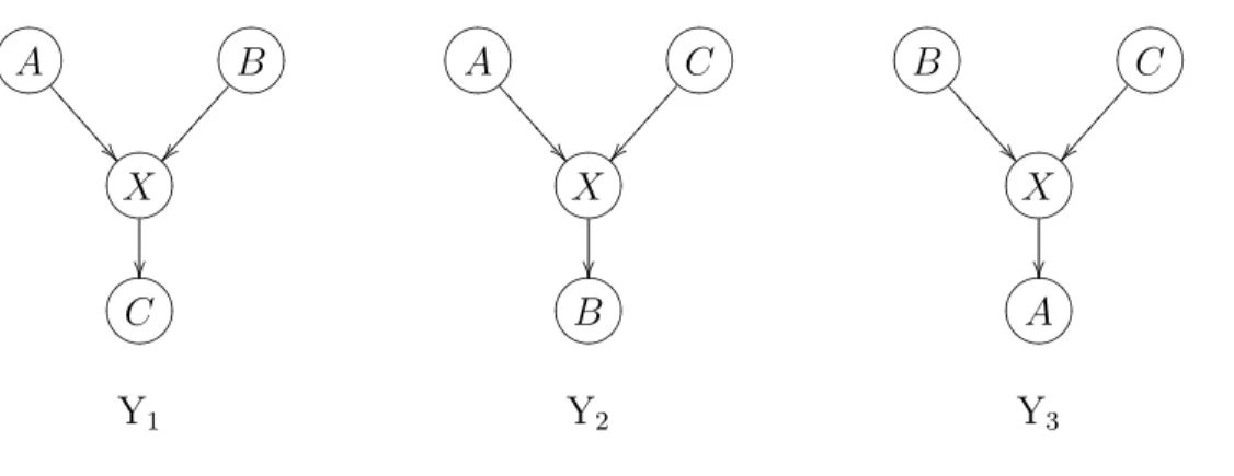
29 Node X and three nodes from the Markov Blanket ofX give rise to three “Y” patterns—Y1, Y2, and Y3. . . 77
30 Prior knowledge (Y is a root node) applied to the models from Figure 25. . . 81
31 Prior knowledge (W1 and W2 are root nodes) applied to the models from Fig-ure 25. . . 82
32 Two Mshielded “Y” structures (“Y1” and “Y2”) and one unshielded “Y” struc-ture (“Y3”). . . 85
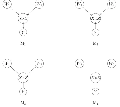
33 Causal models for bounding the causal effect of X on Y. X×Z denotes the cartesian product of X and Z. . . 87
34 An Mshielded “Y” structure (“Y1”) and two confounded “Y” structures (“Y2” and “Y3”). . . 91
35 A causal Bayesian network structure with six nodes and seven arcs. . . 94
36 A causal Bayesian network structure with six nodes and five arcs. . . 95
37 A Y structure. X →Y is a Y arc (YA). . . 96
38 Six “Y” structures. . . 108
39 Three additional “Y” structures. . . 109
41 Hailfinder: Precision versus recall plot.. . . 120
42 Barley: Precision versus recall plot. . . 121
43 Pathfinder: Precision versus recall plot. . . 122
44 Munin: Precision versus recall plot. . . 123
45 BLCD and LCD precision results on the Infant data. . . 133
45.1 BLCD Precision . . . 133
45.2 LCD Precision . . . 133
46 BLCD and LCD recall result on Infant data. . . 134
46.1 BLCD Recall . . . 134
46.2 LCD Recall . . . 134
47 OR and PC precision and recall result on Infant data. . . 135
47.1 OR . . . 135
47.2 PC . . . 135
48 Pair categorization for Pathfinder and Munin . . . 142
48.1 Pathfinder node pair categories . . . 142
48.2 Munin node pair categories . . . 142
49 A Y structure. . . 160
50 A Y PAG. . . 164
51 An unshielded collider X . . . 166
52 A shielded collider X . . . 166
53 A non-collider X . . . 167
54 Another example of a non-collider X . . . 167
PREFACE
We are always searching for causes and effects. My hope is that this research will shed light and provide guidance for this task. I dedicate this dissertation to all my teachers from grade school to grad school who opened the doors and windows of inquiry for me.
First and foremost, I would like to express my gratitude to my advisor professor Greg Cooper for his guidance through the twists and turns of this research. I also sincerely thank my other committee members professor Peter Spirtes, professor Bruce Buchanan and professor Mike Wagner for helpful discussions and critical feedback. I express my gratitude to Dr. Christoph Lehmann and Dr. Michael Neufeld for grading the output of the algorithms obtained from the Infant dataset. I would also like to convey my special thanks to Dr. Joseph Ramsey for help with the latest version of the Tetrad program.
I recall with great appreciation the interesting discussions with my friends and fellow students, in particular, Changwon Yoo and Mehmet Kayaalp that provided an enthusiastic backdrop to pursue my research.
I take this opportunity to thank the National Library of Medicine and the Mellon foun-dation for fellowship support. Finally, my heartfelt thanks go to my family for making this possible.
1.0 WHY CAUSAL DISCOVERY?
1.1 INTRODUCTION
Seeking causes for various phenomena is a significant part of human endeavor. It has been pointed out that “Causality is explanation” (Salmon, 1997), and explanation contributes to understanding. Consider the phenomenon of ozone layer depletion. Scientists studying the ozone layer need to measure the magnitude of loss over time, generate causal postulates and verify them. An ideal approach will involve not only identification of mechanisms responsible for the effect, but also intervention so as to arrest and maybe reverse the trend. Causality is the key to this understanding. Causal knowledge aids planning and decision making in almost all fields. For example, in the domain of medicine, determining the cause of a disease helps in prevention and treatment.
To make the world a better place to live, causal knowledge is the key. Causal knowledge has the potential to tell us the effects of manipulation of the world. It provides explanation for observed phenomena based on past interventions and assessment of outcomes. Causal knowledge also gives us the insight to understand the concurrent causal mechanisms acting in a domain enabling us to plan manipulations or interventions with desirable outcomes. In other words, we will be able to predict the effects of changing (manipulating) nature based on causal knowledge.
As a modern example, discovering causal influences is of paramount importance in sys-tems biology. By syssys-tems biology, we refer to the paradigm shift currently occurring in bi-ology. Instead of just studying single genes and proteins, researchers are investigating whole genomes and proteomes. The advances being made in genomics, proteomics, and metabolic pathways research are contributing to this change. The completion of the human genome
project, the development of the various types of microarray platforms for mRNA expression patterns, protein chips, and other technologies for studying biomolecules are generating a deluge of biological data. This calls for newer methods and algorithms to understand the data. Traditional ways of concentrating on one gene or protein may not be enough. A global perspective has to be developed to obtain the “big picture” and this requires addressing both technical and conceptual issues (Lander, 1999). To accomplish the goals of systems Biology we have to understand the complex causal interactions in the genome and the proteome.
Well designed experimental studies, such as randomized controlled trials, are typically employed in assessing causal relationships. Classically, the value of the variable postulated to be causal is set randomly and its effects are measured. These studies are appropriate in certain situations, for example, animal studies and studies involving human subjects that have undergone a thorough procedural and ethical review.
Based on meta analysis of randomized (experimental) and nonrandomized (observational) studies in healthcare, researchers have found marked correlation between the observational and experimental studies (Benson & Hartz, 2000; Ioannidis et al., 2001). Benson and Hartz focused on clinical studies conducted between 1985 and 1998 and identified more than one hundred published reports related to 19 different treatments. They found that only two of the nineteen treatments had a difference in outcome that was statistically significant between experimental and observational studies (Benson & Hartz, 2000). Ioannidis and others did a larger survey looking at published studies between 1966 and 2000 covering 45 diverse topics based on 240 clinical trials. They found a good correlation between randomized and nonrandomized studies. However, they also noted differences in seven areas that could not be explained by chance (Ioannidis et al., 2001).
Though it is not clear if these findings related to healthcare are generalizable to other areas of inquiry, the potential for observational data as a valid source for discovery science is reinforced by these studies. Observational data is passively and non-invasively collected in routine settings. There is no controlled experimental manipulation of domain variables for data collection. Census data, vital statistics, most business and economic data, astronomical data (e.g., satellite imagery data) and healthcare data routinely collected are some common examples of observational data. Since experimental studies involve deliberate manipulation
of variables and subsequent observation of the effects, they have to be designed and executed with care and caution. Experimental studies may not be feasible in many contexts due to ethical, logistical, or monetary cost considerations. These practical limitations of experi-mental studies heighten the importance of exploring, evaluating and refining techniques to learn more about causal relationships from observational data. The goal is not to replace experimental studies, which are extremely valuable in science, but rather to augment, refine and guide experimental studies when feasible. If pointers to interesting causal relationships could be obtained from observational studies, those causal influences could be more rigor-ously tested and evaluated in experimental settings more efficiently. In those areas of inquiry where experimental studies are not possible or feasible, then causal insight may need to rely primarily on observational data.
Moreover, we need discovery methods and efficient algorithms that will scale up to handle the enormous amounts of data generated continuously in diverse domains. The efficiency and scalability requirements lead us to the following hypothesis for causal hypothesis.
1.2 HYPOTHESIS FOR CAUSAL DISCOVERY
Before stating our hypothesis formally we introduce some definitions and provide a context C for causal data mining.
Large datasets Datasets from which it is not feasible to learn a global causal model us-ing limited computational resources (defined below). The following datasets would be considered as large datasets for our study purposes.
1. Datasets with more than hundred variables or more than ten thousand records. Examples include vital statistics records, multi-center studies, and clinical patient records in medical centers.
2. Datasets with more than one thousand variables, such as gene expression datasets.
Anytime framework A context in which an anytime algorithm would be useful. An any-time algorithm has the property of progressively improving its results over any-time. These
algorithms are usually controlled by a meta-level decision procedure to evaluate the out-put and to stop or continue the comout-putation (Russell & Norvig, 1995, page 844).
Local search (LS) In this dissertation research the focus of a local search methodology is on discovering submodels (subgraphs) of the causal Bayesian network generating the data (for example, pair-wise causal relationships, a node and its parents (direct causes), a node and its children (direct effects)), rather than attempting to build a global causal model. The LS considers a small subset of the total number of variables—for example, triplets or quads of variables at one time. The LS also incorporates other background knowledge in the form of priors. The priors could be special (“W”) variables, a temporal ordering of the variables in the dataset, or already known pair-wise causal relationships.
Limited computational resources Limited processor speed, main memory and running time. A typical current example would be a PC with a 3 GHz processor speed, 1 GB RAM, and a run time of two weeks.
Validity In this dissertation research validity of an output is thedegreeto which a relation-ship is causally correct in some context. For causal discovery algorithms, validity of the output can be assigned based on how it compares to a reference standard. Validity can be studied by categorizing it into three different types—content, criterion-related and construct.
The content validity of an algorithm can be ascertained by the underlying theory, as-sumptions and the correctness of the algorithm. If the underlying theory is sound, the assumptions are correct, and there is a proof of correctness for the algorithm, content validity can be assigned. This is the most basic concept of validity and is also known as “face” validity.
Criterion-related validity can be assessed by comparing the output of the algorithm to a reference gold standard.
Construct validity is similar to criterion-related validity but needs a more sophisticated and rigorous approach (Friedman & Wyatt, 1997). For example, evaluation of a potential “causal” output can be confirmed by a randomized controlled trial.
In general, validity can be defined subjectively by the expert user based on his knowledge of the domain. The validity scale could be qualitative or quantitative.
Better Performance For grading the performance of a causal discovery algorithm the focus will be on causal structure. The performance will be primarily assessed using simulated data from expert designed causal networks as the true structure is known and hence the performance of the algorithm can be assessed as a function of the true positives, false positives, true negatives, and false negatives.
In particular the following two metrics will be computed for the output of the algorithm:
P recision= T P O
T O (1.1)
Recall= T P O
T P (1.2)
where T P O is the Total number of true positive relationships output, T O is the Total number of relationships output, andT P is theTotal number of true positive relationships in the network.
Better performance is defined as higher precision and higher recall.
The context C for our causal data mining hypothesis incorporates the following features: 1. Large datasets.
2. An anytime framework.
3. Limited computational resources.
Hypothesis: Causal discovery using local search methods in context C will have bet-ter performance compared to the causal discovery methods using global search described in Chapter 3.
2.0 BACKGROUND: FRAMEWORK FOR CAUSAL DISCOVERY
Information technology (IT) is at the forefront of increasing data generation and storage which has resulted in the availability of larger and larger datasets in various domains. It is important to have efficient andanytimeapproaches to discover meaningful patterns in these large volumes of data using available computational resources. This dissertation addresses this issue from the perspective of discovering causal relationships.
This section is organized as follows. We first provide a brief introduction to Bayesian networks (BN) in Section2.1 and causal Bayesian networks (CBN) in Section2.2. We define and discuss “causal influence” in Section 2.3, and introduce the basic assumptions used for causal discovery in Section 2.4. Bayesian scoring of causal Bayesian networks is discussed in Section 2.5. Bayesian model averaging takes model uncertainty into account rather than assume that a single model is correct. It is described in Section 2.6. Section 2.7 discusses selective Bayesian model averaging and model selection for causal discovery. Section 2.8
describes the method we use for handling missing data in practice.
2.1 BAYESIAN NETWORKS
Our framework for causal discovery is founded on Bayesian networks. BNs are directed acyclic graphs (DAGs) with the vertices (nodes1) representing observed variables in a domain
and the directed edges denoting dependence relationships between the variables. The prob-abilistic relationships among the variables represented in a BN are quantified by marginal probabilities (for root nodes) and conditional probabilities (for non-root nodes). The joint
probability distribution of the variables represented in a domain can be expressed compactly using a BN and can be factorized as follows:
P(X1, X2, . . . , Xn−1, Xn) = n Y i=1 P(Xi|Pa(Xi)) (2.1) where:
• X1, X2, . . . , Xn−1, Xn are the vertices of the BN.
• Pa(Xi) denotes the set of parents of the node Xi in the BN (Xj is a parent ofXi iff there
is a directed edge from Xj to Xi).
See (Neapolitan, 1990; Pearl, 1991; Heckerman, 1996) for more details.
Our focus is on learning causal Bayesian networks (see Section 2.2) from data and the natural question is why should we try to learn these models from data. Initially Bayesian networks were built as knowledge-based systems. The structure and the parameters were specified by experts (Beinlich et al., 1990; Andreassen et al., 1987; Heckerman et al., 1992). It was very labor intensive and challenging for experts to specify precisely the prior and conditional probabilities that parameterized the models. For various domains, experts had problems assessing a full-fledged causal structure, or the parameters, and in some situations both. Hence researchers started to focus on data—initially for parameter estimation, but subsequently to learn both the network structure as well as the probabilities associated with it.
2.2 CAUSAL BAYESIAN NETWORKS
A causal Bayesian network (orcausal networkfor short) is a Bayesian network in which each arc is interpreted as a direct causal influence between a parent node (variable) and a child node, relative to the other nodes in the network (Pearl, 1991). For example, if there is a directed edge from A toB (A−→B), nodeA is said to exert a causal influence on nodeB. Figure 1illustrates the structure of a hypothetical causal Bayesian network structure, which
ONML HIJKX1 ~ ~|||| |||| | Ã Ã B B B B B B B B B History of Smoking Chronic
BronchitisONMLHIJKX2
à à A A A A A A A A A A ONMLHIJKX3 ~ ~}}}} }}}} }} à à A A A A A A A A A A Lung Cancer
Fatigue ONMLHIJKX4 ONMLHIJKX5 Mass Seen onChest X-ray
Figure 1: A hypothetical causal Bayesian network structure
contains five nodes. The states of the nodes and the probabilities that are associated with this structure are not shown.
The causal network structure in Figure 1indicates, for example, that aHistory of Smok-ing can causally influence whetherLung Cancer is present, which in turn can causally influ-ence whether a patient experiinflu-ences Fatigueor presents with a Mass Seen on Chest X-ray.
Theindependence mapor I-map of a causal network is the set of dependence/independence relationships between individual variables or sets of variables unconditioned or conditioned on other variables or sets of variables. The I-map of the causal network W1 −→ X ←−W2
is as follows: • W1⊥⊥W2 • W16⊥⊥X • W16⊥⊥X|W2 • W16⊥⊥X • W26⊥⊥X|W1 • W16⊥⊥W2|X
2.3 CAUSAL INFLUENCE, CONFOUNDED AND UNCONFOUNDED CAUSAL RELATIONSHIPS
We define thecausal influenceof a variableX on variableY using themanipulation criterion (Spirtes et al., 1993; Glymour & Cooper, 1999). The manipulation criterion states that if we had a way of setting just the values of X and then measuring Y, the causal influence of X
onY will be reflected as a change in the conditional distribution of Y. That is, there exists values x1 and x2 of X such that P(Y| set X =x1)6=P(Y| setX =x2). We now introduce
the types of causal influences (relationships) encountered in our framework.
In a causal Bayesian network an arc between any pair of nodes represents a causal influence. These causal relationships can be termed as confounded or unconfounded based on the following criteria. The arcs and node pairs can be categorized using the following framework. Each pair (X,Y) is categorized as follows:
Causal and unconfounded pair (CUP) If CUP(X,Y), then there is a directed path from X to Y, and there is no common ancestor W that has a directed path to X and a directed path to Y that does not traverse X. A directed path from node X to node Y
is a set of one or more directed edges originating from X and ending in Y. The nodes Lung Cancer and Mass seen on Chest X-ray in Figure 1 are causal and unconfounded, that is CUP(X3,X5) holds.
Causal and confounded pair (CCP) If CCP(X,Y) holds then there is a directed path from X to Y, and there is a common ancestor W that has a directed path to X, and a directed path to Y that does not traverse X. The nodes Chronic Bronchitis and Fatigue in Figure 1 are causal and confounded (History of Smoking is a common ancestor).
For completeness we now introduce the two other types of relationships encountered between two variables X and Y in a causal Bayesian network.
Confounded-only pair (COP) There is no directed path between X and Y, and there is a common ancestor Wthat has a directed path toX, and a directed path to Ythat does not traverse X. The nodes Chronic Bronchitis and Lung Cancer in Figure 1 have the confounded-only pair relationship.
Independent pair (IP) There is no d-connecting path (Pearl, 1991) between X and Y. See Section 3.1.1 for an explanation of d-separation and d-connectivity.
The arcs of a CBN can be categorized as given below:
Causal and unconfounded arc (CUA) If CUA(X,Y), then there is an arc fromXtoY, and there is no common ancestor W that has a directed path to X and a directed path to Y that does not traverse X. The arc between Lung Cancer and Mass seen on Chest X-ray in Figure1 is causal and unconfounded, that is CUA(X3,X5) holds.
Causal and confounded arc (CCA) If CCA(X,Y), then there is an arc from X to Y, and there is a common ancestor Wthat has a directed path to X and a directed path to Y that does not traverseX. The arc between Chronic BronchitisandFatigue in Figure1
is causal and confounded (History of Smoking is a common ancestor).
Note that all causal and unconfounded arcs (CUA) are causal and unconfounded pairs (CUP) but not vice versa. Likewise, all causal and confounded arcs (CCA) are causal and confounded pairs (CCP) but not vice versa. Note also that there cannot exist confounded-only or independent arcs.
In causal discovery, we are usually interested in identifying both confounded (usually by a measured variable) and unconfounded causal relationships. Consider the three hypothetical models in Figure 2. Assume that G stands for a Gene, S for Smoking, and C for Cancer, and these variables have two states—present and absent. Note that H stands for a hidden variable. Model (1) has the measured confounder G, Model (2) has a hidden (unmeasured) confounder H, and Model (3) is unconfounded. Model (1) and model (3) are informative. For example, ifGis causing a section of the population to smoke and also causing lung cancer (C), an effective intervention strategy could be to focus on the segment of the population without G and persuade them to stop smoking. Likewise, advocating cessation of smoking is a good interventional strategy to reduce the incidence of lung cancer based on model (3). The causal effect of S onC can be assessed from observational data. Model (2) is a lot less informative. Because of the hidden confounder H, the causal effect of S on C cannot be quantified with confidence from observations (not interventions) of S and C only.
rela-7654 0123G ¢ ¢¥¥¥¥ ¥¥ À À ; ; ; ; ; ; 7654 0123S //76540123C (1) 7654 0123H ¢ ¢¥¥¥¥ ¥¥ À À ; ; ; ; ; ; 7654 0123S //76540123C (2) 7654 0123S //76540123C (3)
Figure 2: Three hypothetical causal models in which S causes C. S and C are confounded by a measured variable represented byGin Model (1), and a hidden confounderH in Model (2). There is no confounding variable (measured or hidden) in Model (3).
tionships of the form “X does not causally influence Y”. However, for purposes of this dissertation we concentrate on causal discovery and do not focus on acausal discovery.
2.4 ASSUMPTIONS FOR CAUSAL DISCOVERY
In this section we describe the basic assumptions of our causal discovery framework. Ad-ditional assumptions that some causal discovery algorithms may require will be introduced with the respective algorithm descriptions.
2.4.1 The causal Markov condition
The causal Markov condition (CMC) gives the independence relationships2 that are
specified by a causal Bayesian network:
A variable is independent of its non-descendants (i.e., non-effects) given just its parents (i.e., its direct causes).
According to the causal Markov condition, the causal network in Figure1is representing that the chance of a Mass Seen on Chest X-raywill be independent of aHistory of Smoking, given that we know whether Lung Canceris present or not.
The CMC is representing the “locality” of causality. This implies that indirect (distant) causes become irrelevant when the direct (near) causes are known. For example, if we know the status of Lung Cancer (present/absent), knowledge of History of Smokingdoes not give any additional information to enhance our understanding of the effect variable (Mass seen on chest X-ray). The CMC can fail in certain situations as illustrated by the following two examples adapted from (Cooper, 1999).
Consider the hypothetical CBN in Figure 3. If we sum over and marginalize out the
X2, we get the CBN shown in Figure4. This demonstrates that the absence of a statistical
dependency between two variablesXandY does not necessarily mean that there is no causal relationship between them when hidden variables are also considered.
High Blood Cholesterol : no, moderate, severe
Coronary Artery Disease : absent, moderate, severe
Myocardial Infarction : absent, present
Figure 5shows a CBN that depicts the following hypothetical causal relationships: High Blood Cholesterol causally influences Coronary Artery Disease which in turn causally influ-ences Myocardial Infarction. Each of these variables take one of the corresponding values given above.
Assume that the CMC correctly implies thatX1 and X3 are independent given X2. Now
consider the variables and their states where Coronary Artery Diseasetakes values “absent” 2We use the termsindependenceanddependencein this section in the standard probabilistic sense.
High
Cholesterol ONMLHIJKX1
Á Á = = = = = = = = = ONMLHIJKX2 ¡ ¡¢¢¢¢ ¢¢¢¢ ¢ Gene ONML HIJKX
3 Heart DiseaseIschemic
P(X1=present) = 0.5 P(X2=present) = 0.5
P(X3=present) |X1=present,X2=present)=0.1 P(X3=present)|X1=present,X2=absent)=0.9 P(X3=present)|X1=absent, X2=present)=0.9 P(X3=present)|X1=absent,X2=absent)=0.1
Figure 3: A CBN with three nodes X1, X2, and X3. [Modified from (Cooper, 1999)]
and “present” instead of the three level given earlier. If we now condition on the value Coronary Artery Disease = present, it is possible that X1 may not be independent of X3.
A “severe” High Blood Cholesterol causes “severe” Coronary Artery Disease that in turn causes myocardial infarction. In this scenario, knowledge that “Coronary Artery Disease = present” does not renderHigh Blood CholesterolandMyocardial Infarction independent (see Figure 6).
This example shows that the independence properties of a CBN implied by the CMC may vary if the number of states of one or more variables in the CBN is modified (Cooper, 1999).
Another point worth noting is that based on quantum theory causality is not local (Her-bert, 1985; Cooper, 1999) and this may cause CMC to fail. However, we note that as with Einsteinian physics not negating Newton’s laws in the macroscopic world, local conditioning given by CMC is not generally negated by quantum mechanics in the macro world.
High
Cholesterol ONMLHIJKX1 P(X1=present)=0.5
Ischemic
Heart DiseaseONMLHIJKX3 P(X3=present)=0.5
Figure 4: A CBN with two nodesX1, and X3. [Modified from (Cooper, 1999)]
2.4.2 The causal faithfulness condition
While the causal Markov condition specifies independence relationships among variables, the
causal faithfulness condition(CFC) specifies dependence relationships:
Variables are dependent unless their independence is implied by the causal Markov condi-tion.
For the causal network structure in Figure 1, three examples of the causal faithfulness condition are (1) History of Smoking and Lung Cancer are probabilistically dependent, (2) History of Smoking and Mass Seen on Chest X-ray are dependent, and (3) Mass Seen on Chest X-rayandFatigueare dependent. The intuition behind that last example is as follows: the existence of a Mass Seen on Chest X-ray increases the chance of Lung Cancer which in turn increases the chance of Fatigue; thus, the variables Mass Seen on Chest X-ray and Fatigueare expected to be probabilistically dependent. In other words, the two variables are dependent because of a common cause (i.e., a confounder).
The CFC is related to the notion that causal events are typically correlated in obser-vational data. The CFC relates causal structure to probabilistic dependence. The CFC generally holds in most situations but it can also fail. The following discussion and examples are based on (Cooper, 1999).
ONML
HIJKX1 //ONMLHIJKX2 //ONMLHIJKX3
High Cholesterol Coronary Artery Disease Myocardial Infarction
High Blood Cholesterol : no, moderate, severe
Coronary Artery Disease : absent, moderate, severe
Myocardial Infarction : absent, present
Figure 5: A CBN with three nodes X1, X2, and X3. [Modified from (Cooper, 1999)]
2.4.2.1 The problem of deterministic relationships Assume that all the variables in Figure 7are binary and the probability distributions are as follow:
P(X1=yes) = 1 P(X2=yes |X1=yes) = 1 P(X2=no |X1=no) = 1 P(X3=yes |X2=yes) = 1 P(X3=no |X2=no) = 1 ONML
HIJKX1 //ONMLHIJKX2 ''//ONMLHIJKX3
High Cholesterol Coronary Artery Disease Myocardial Infarction
ONML
HIJKX1 //ONMLHIJKX2 //ONMLHIJKX3
Figure 7: A CBN with three nodes X1, X2, and X3.
Note that all the three variables X1,X2, and X3 are related in a deterministic way. All
the three variables are always in the state “yes”. Since all the values are the same (yes), we cannot infer from observational data the potential effect of a manipulation.
Now assume that P(X1=yes) = 0.5. All the conditional probabilities remain the same.
Knowing the value of X3 tells us the value of X1 and conditioning on X2 has no effect.
In both these situations CFC is violated. We also emphasize that a deterministic rela-tionship is not a necessary condition for the violation (see Figure 3).
2.4.2.2 Goal oriented systems A class of systems where CFC can fail is the framework of goal oriented systems. Consider the clinical situation represented by Figure 8. H stands
Disease GFED @ABCH ( ( Q Q Q Q Q Q Q Q Q Q Q Q Q Q Q Q Q v vmmmmmm mmmmmm mmmmm ONML
HIJKX1 //ONMLHIJKX2 //ONMLHIJKX3
Patient Symptom Physician Treatment Patient Outcome
Figure 8: A CBN with three observed nodes—X1,X2,X3, and one hidden nodeH. [Modified
from (Cooper, 1999)]
for a hidden disease. Assume that it is a slow-growing tumor that turns malignant in a proportion of patients and gives rise to symptoms. The disease is fatal only when it turns malignant and left untreated. Once patients develop symptoms they consult a physician,
get treatment (say chemotherapy) and go into remission. If the outcome variable is five-year survival and all patients survive, physician action (X2) and patient outcome (X3) will be
independent. This violates the CFC. But the CFC is likely to hold in systems that are not goal-oriented. The CFC is also likely to hold in goal-oriented systems if the goal is to keep a constant state of the system. Otherwise, the CFC is not likely to hold in goal oriented systems.
When we consider exhaustively all possible distributions the proportion that violate CFC are relatively very small (Spirtes et al., 1993; Meek, 1995). But such distributions when they exist can cause problems in discovering causal relationships using algorithms that assume CFC (Cooper, 1999).
Before we move on to the next property of a CBN, we introduce our notational convention. We represent sets of variables in bold and upper case, random variables by upper case letters italicized, and the value of a variable or sets of variables by lower case letters. When we say
X = x, we mean an instantiation of all the variables in X, while X = x denotes that the variable X is assigned the value x. Graphs are denoted by calligraphic letters, such as G or upper case letters such as G or M.
We now describe another property of a CBN that is based on the Markov property. This property is called theMarkov Blanket(MB). The MB of a nodeX in a CBNG is the union of the set of parents ofX, the children ofX, and the parents of the children ofX (Pearl, 1991). Note that it is the minimal set of nodes when conditioned on (instantiated) that makes a nodeX independent of all the other nodes in the CBN. The MB is minimal and unique when there are no deterministic relationships in the CBN. Let V be the set of all variables in G,
B the MB of X, and A be V\(B∪X). Conditioning on B renders X independent of A. For example, in the hypothetical CBN shown in Figure 1, the MB of node X4 is composed
2.5 BAYESIAN SCORING OF COMPLETE CAUSAL MODELS
Bayesian methods for scoring CBNs were first developed by Cooper and Herskovits (Cooper & Herskovits, 1992). Subsequently a modified scoring metric was proposed by Heckerman et al. (Heckerman et al., 1995). Starting with a set of user-specified priors for network structures and parameters, the methods derive a posterior score using observational data and some basic modeling assumptions. Instead of user-specified priors, the methods also allow use of noninformative priors for both structures and parameters.
We now summarize the Bayesian scoring of a network structure. This discussion is based on (Cooper, 1999, pages 39–40). Let D be a dataset over a set of observed variables V. Let
BS represent any arbitrary causal BN structure overV andKdenote background knowledge
that has bearing on the causal network overV. We can derive the posterior probability of a BN structure BS as follows: P(BS|D,K) = P(BS, D|K) P(D|K) = P(BS, D|K) P BSP(BS, D|K) (2.2)
Since P(D|K) is a constant for all the causal structures, we can write equation 2.2 as:
P(BS|D,K)∝P(BS, D|K) (2.3)
The right hand side of equation 2.3 can be expressed as:
P(BS, D|K) = P(BS|K)P(D|BS,K)
= P(BS|K) Z
P(D|BS, θBS,K)P(θBS|BS,K)dθBS (2.4)
where P(BS|K) is the prior probability of BS given the background knowledge K that we
possess;θBS represent the parameters associated with the BN structureBS;P(D|BS, θBS,K)
is the likelihood of data Dassuming the network structureBS, its parameterizationθBS and
background knowledge K; and P(θBS|BS,K) is the prior for the parameterization of the
2.6 BAYESIAN MODEL AVERAGING (BMA)
IfX and Y represent a pair of variables in V, we can derive the posterior probability of the existence of a causal relationship X → Y using Bayesian model averaging over structures containing X →Y:
P(X →Y|D,K) = X
BSX→Y
P(BSX→Y|D,K) (2.5)
whereBSX→Y denotes a causal BN structure with the causal relationshipX →Y. Combining
equation 2.2 through equation 2.5, we can write:
P(X →Y|D,K) = P BSX→Y P(BSX→Y|K) R P(D|BSX→Y, θBSX→Y,K)P(θBSX→Y|BSX→Y,K)dθBSX→Y P BSP(BS|K) R P(D|BS, θBS,K)P(θBS|BS,K)dθBS (2.6)
The numerator sum (PB
SX→Y) is over the BN structures containing the causal
relation-ship X → Y, and the denominator sum (PBS) is over the BN structures being modeled. Note that this derivation of posterior probability of a causal relationship is exhaustive and comprehensive. However, it often is not computationally feasible in the exact form shown.
The model BS can be scored using a Bayesian metric such as the K2 metric (Cooper
& Herskovits, 1992) or the BDe metric (Heckerman et al., 1995). Using these metrics the integrals in Equation 2.6 can be computed.
2.7 SELECTIVE BAYESIAN MODEL AVERAGING AND MODEL
SELECTION
The number of causal DAGs is exponential in the number of variables in the DAG. For any non-trivial domain, scoring and summing over all these models in the framework of BMA is computationally intractable. This calls for identifying a much smaller subset of models that has the potential to be high-scoring. Cooper and Herskovits (Cooper & Herskovits, 1992) describe a greedy heuristic search method to restrict the number of models by limiting the
number of parents of each node. This greedy forward search can be used to arrive at a single highest scoring model in which case it is termed model selection. The search strategy can also be used to select a set of high scoring models. Another method is restricting the search to Markov equivalent class of models (Spirtes & Meek, 1995).
Since in our dissertation we learn local (composed of a subset of variables) causal models we do not limit our search to just a few of the possible CBNs over the modeled variables. Instead of restricting the scoring to Markov equivalent class of models, we score all the models that are causally distinct as discussed in Section 5.1.
2.8 HANDLING MISSING DATA
Data is said to be missing when values for observed variables are not available for a subset of instances. A variable is considered hidden when its value remains unmeasured for all the instances. See Heckerman et al. (Heckerman et al., 1999, pages 151–153) for a description of Bayesian scoring methods in the presence of missing data and hidden variables. Since an exact Bayesian approach is often intractable, approximation methods such as Gibbs sampling (Geman & Geman, 1984), Gaussian approximation, and maximum likelihood approximation with EM algorithm are often used. As the focus of this dissertation is not in developing methods for handling missing data, we now describe a practical and simple method that we propose to follow.
With simulated data the problem of missing data is normally not encountered. However, with most real-world datasets missing data is often present. The absence of an observation could be random or dependent on the actual states of the variables. For purposes of this discussion we assume that data is missing completely at random. Researchers have used different approaches to the problem of missing data. A simple approach is to discard instances with missing data. However, this could result in a substantial reduction in sample size. For the algorithms in our prior work, we excluded instances that had a missing value in any of the three attributes considered by the algorithm at a particular time. We propose to follow the same approach for a newly introduced algorithm (BLCD), as only a subset of
the variables are considered by the algorithm for its local search strategy (See Section 5.1
for details). However, the PC and FCI algorithms consider all the variables in assessing a causal relationship. Thus excluding all those instances with missing values is not a feasible approach as little or no instances would remain. We propose to take the simple approach of treating the missing value as a separate state of an attribute. For example, if a variable
X has known values “Y” and “N”, the missing value is assigned “U” (unknown). This can lead to missing causal relationships but not incorrectly claiming causal influences. We refer to this phenomenon as the missing value effect. However, this adds to the computational complexity as the number of states of each variable that has even a single missing value increases by one. This increase in the number of states of variables results in larger marginal and conditional probability tables for parameter estimation.
3.0 RELATED WORK: LEARNING CAUSAL BAYESIAN NETWORKS FROM DATA
In this chapter we review the current Bayesian network learning algorithms that are useful for discovering causal structure from data. Note that some of the algorithms reviewed do not make explicit “causal” claims. Others do so, and we describe them in greater detail.
The BN learning methods can be broadly classified into constraint-based and Bayesian. The networks have a structural component and a parametric component that represents marginal and conditional probabilities of the variables. Once the structure is ascertained, it is often straightforward to estimate the parameters from data particularly in the absence of hidden confounders. Hence our focus here will be on search methods for learning the causal structure from data.
Constraint-based methods use tests of independence/dependence between two variables (X, Y) or two sets of variables (X, Y) given another set of variables (Z) (including the empty set) to add/remove edges between variables and orient them. They typically start with a complete network and delete edges based on the tests, or start with a fully disconnected network and add edges, or do both. The number of possible tests to be done in this framework is exponential in the number of variables V in the worst case.
Score-based methods compute the probability of the data D given a structure. Exhaus-tive model selection involves scoring all possible network structures on a given set of variables and then picking the structure with the highest score. However, heuristic search methods are typically employed to restrict the search space as the number of potential networks are exponential in the total number of variables. Researchers have proved that it is NP-hard to identify a Bayesian network that can have up to k parents for a node where k ≥ 1 and a score greater than some constant C using a likelihood equivalent score such as the BDe
metric (see Section 3.2.4) (Chickering, 1996).
A different class of score-based methods are based on the minimal description length (MDL) principle that has its roots in information theory. These are described in Section3.5. All the causal discovery algorithms discussed below make two cardinal assumptions—the causal Markov and the causal faithfulness conditions, which are described in Section 2.4. Additionally, constraint-based algorithms make use of statistical tests for elucidating de-pendence and indede-pendence between variables or sets of variables. Hence they also need a statistical testing assumption. This is discussed in Section 3.4.1.
The causal Bayesian network (CBN) learning methods can also be classified as global or local based on their search methodology and their output. If the goal is to learn a unified CBN over all the model variables, the search methodology is termed global. PC and FCI are global constraint-based algorithms (Spirtes et al., 1993). If the goal of the learning procedure is to discover causal models on subsets of the model variables (for example, pairwise causal relationships), alocal searchmethodology is employed. This could be over triplets of variables (restricted local search) such as in LCD (see Section 3.4.1) or over more than three variables (extended local search) such as in BLCD (see Section 5.1).
3.1 GLOBAL CONSTRAINT-BASED ALGORITHMS
In this section we discuss the PC, FCI, anytime FCI and the GS Markov blanket algorithm.
3.1.1 PC algorithm
The PC algorithm takes as input a dataset D over a set of random variables V, a condi-tional independence test, and an α level of significance threshold for the test. It then out-puts an essential graph that we define below. Recall that Markov equivalence (also known as independence equivalence) is a relationship based on independence that establishes an equivalence class of directed acyclic graphs over an observed set of variablesV. These DAGs are statistically indistinguishable based on independence relationships among V. Let U be
one equivalence class of DAGs over V. An essential graph E of U over V will have directed and undirected edges such that each directed edge between a pair of nodesX andY will be represented in all the DAGs in U and each undirected edge between a pair X and Y in E will be represented as either X → Y or X ← Y in all the DAGs in U (Cooper, 1999) with both arc types represented.
We first define the terms ancestor and descendent. We then introduce the concept of a d-separating set and outline the steps of the algorithm.
Ancestor : In a CBN, node X is said to be an ancestor of node Y if there is a directed path from X toY.
Descendent : In a CBN, nodeY is said to be a descendent of nodeX is there is a directed path from X toY. GFED @ABCV 1 ² ² GFED @ABCV2 ~ ~~~~~ ~~~~ ~ GFED @ABCV3 Ã Ã @ @ @ @ @ @ @ @ @ GFED@ABCV4 ~ ~~~~~ ~~~~ ~ GFED @ABCV 5 ² ² GFED @ABCV 6
Figure 9: A hypothetical Bayesian network structure
d-separation (Pearl, 1991): Consider the DAG G in Figure 9. Assume that X and Y are vertices in GandZis a set of vertices in Gsuch thatX6∈ZandY 6∈Z. X andY are said to be d-separated given Ziff the following property holds: there exists noundirected path1 U betweenX andY s.t.
1An undirected path between two verticesAand B in a graphGis a sequence of vertices starting with
A and ending withB and for every pair of vertices X andY in the sequence that are adjacent there is an edge between them (X→Y orX ←Y) (Spirtes et al., 2000, page 8)
1. every collider2 on U has a descendant inZ.
2. no other vertex onU is inZ.
Likewise, if X and Y are not in Z, then X and Y are d-connected given Z iff they are not d-separated given Z.
In Figure 9 the nodes V1 and V6 are d-separated by V3. The nodes V1 and V4 are d-connected given V6.
The following are the salient steps of the PC algorithm (Spirtes et al., 2000, page 84–85).
1. Start with complete undirected graph composed of all the variables as vertices.
2. For each pair of variables, obtain a minimal d-separating set. The set Sj is a minimal
d-separating set of node X and node Y among all the d-separating sets Si if |Sj| ≤ |Si|
for all Si6=j. For example, for the pair (X, Y), try to find the minimal conditioning set of
nodes S(including the empty set) that satisfies (X⊥⊥Y|S). This is done by starting with low order conditional tests and moving up. Note that we check only subsets of vertices currently adjacent to one endpoint or the other. If such a set Sis found then delete edge
X—Y, whereX—Y represents an undirected edge between X and Y.
3. Consider each triplet of nodes X,Y, andZ where (X, Y) and (Y, Z) are adjacent3 while
(X, Z) is not. If Y is not in the d-separating set of (X, Z), the triplet is oriented as
X →Y ←Z.
4. Orient edges iteratively using the following rules until no more edges can be oriented. • If X →Y and Y—Z are present, and X and Z are not adjacent, then orient (Y —
Z) as (Y →Z).
• If there is a directed path from X to Y, and X—Y exists, then orient X — Y as
X →Y.
• If W → X ←Y and X —Z, and W —Z, and Y — Z, and there is no adjacency between W and Y, then the edge X —Z can be oriented asX ←Z.
The PC algorithm has a worst-case time complexity that is exponential in the largest degree in the output graph. The degree of a vertexv refers to the number of adjacent nodes (vertices) of v. The PC is also known to be unstable in steps 2 and 3 (Spirtes et al., 1993).
2A node with a head to head configuration. Cis a collider in A→C←B.
3Two nodesX andY are said to be adjacent if there is an edge betweenX andY. Initially all pairs of
Note that it is not guaranteed to orient all the edges as the goal is to identify the essential graph. Hence the final output can be a graph with both directed and undirected edges.
PC also makes an assumption of causal sufficiency. This means that all the variables of the causal network are measured and there are no latent or hidden variables. Hence PC is not designed to discover hidden variables that are common causes of any pair of observed variables.
Spirtes et al. have reported that the PC algorithm learned the Alarm network (see Section 6.3.2) from data orienting most of the edges correctly but omitted two edges of the generating graph in one trial and added an extra edge in another (Spirtes et al., 2000, page 109).
The PC algorithm was also evaluated on simulated data from artificially generated CBNs. The algorithm performed well with high sample sizes and a low average degree for the generating graph (Spirtes et al., 2000, page 116).
3.1.2 FCI algorithm
Real world data can contain hidden (unobserved or latent) variables. There are variables in a domain that were unmeasured and hence are not explicitly represented in the collected data. Another problem pertaining to real-world data is sample selection bias. This occurs when the values of the variables under study determine when certain instances are included in the sample (Spirtes et al., 1999). Spirtes et al. introduce the following assumption for data that is subject to sample selection bias.
3.1.2.1 Population inference assumption (Spirtes et al., 1999) The population selected by sampling criteria has the same causal structure (the statistical properties might differ due to sample selection bias) as the population about which causal inferences are to be made.
The FCI algorithm can discover causal relationships in the presence of hidden variables and selection bias. The first three steps of the FCI algorithm are similar to that of the PC algorithm. The later steps involve edge deletion and then orienting the edges using a
different set of rules compared to the PC algorithm. FCI takes as input dataD representing a causal graphical structure that has the observed set of variables O and outputs a partial ancestral graph (PAG) of the causal structure over O (Spirtes et al., 1999).
We introduce some definitions that are required for understanding FCI and anytime FCI (AFCI) based on the description in (Spirtes et al., 2000) and (Spirtes et al., 1999).
1. π refers to a partial ancestral graph.
2. V refers to the set of all variables in a domain. 3. L refers to the set of latent variables in a domain. 4. S refers to the set of selection variables in a domain. 5. O refers to the set all observed variables.
6. A ↔B refers to a hidden cause that directly causesA and B. 7. A◦→B refers to eitherA↔B or A→B.
8. A∗ →B refers to one of A↔B, A→B, A◦→B.
9. B is a collideralong path < A, B, C > iff A∗ →B← ∗C inπ
10. An edge between B and A is into A iff A← ∗B in π. 11. An edge between B and A is out of A iff A→B inπ. 12. T is Sepset(X, Y) ifT d-separates X and Y.
A DAG G with a partition of its variable set V into O, S and L variables is written as
G(O,S,L).
3.1.2.2 O-Equiv(Cond) (Spirtes et al., 1999) A Cond is a set of conditional inde-pendence relations among the variables inO. A DAGG(O,S,L) is inO-Equiv(Cond)when
G(O,S,L) entails that X⊥⊥Z|(Y∪(S=1)) iff X⊥⊥Z|Y is in Cond. If G0(O,S0,L0) entails
thatX⊥⊥Z|(Y∪(S0 =1)) iff G(O,S,L) entails that X⊥⊥Z|(Y∪(S =1)), then G0O,S0,L0)
is in O-Equiv(G).
We now define a partial ancestral graph.
3.1.2.3 Partial ancestral graph (Spirtes et al., 1999) A DAG G with a partition of its variable setV intoO,S andL variables is written asG(O,S,L). A PAGπ represents a DAG G(O,S,L) iff: