FORECASTING EXCHANGE RATE
A Uni-variate out of sample Approach (Box-Jenkins Methodology)
Mahesh Kumar Tambi1
Abstract
In this paper we tried to build univariate model to forecast exchange rate of Indian Rupee in terms of different currencies like SDR, USD, GBP, Euro and JPY. Paper uses Box-Jenkins Methodology of building ARIMA model. Sample data for the paper was taken from March 1992 to June 2004, out of which data till December 2002 were used to build the model while remaining data points were used to do out of sample forecasting and check the forecasting ability of the model. All the data were collected from Indiastat database. Result of the paper shows that ARIMA models provides a better forecasting of exchange rates than simple auto-regressive models or moving average models. We were able to build model for all the currencies, except USD, which shows the relative efficiency of the USD currency market.
Key words: Exchange rate forecasting, univariate analysis, ARIMA, Box-Jenkins methodology, out of sample approach
Object
This paper is an attempt to forecast the exchange rate of Indian rupee (INR) in terms of five different currencies; SDR, USD, GBP, Euro and JPY. Paper tries to make short horizon forecasts based on univariate time series analysis. A survey of literature shows a continuous debate is going on whether exchange rate follows a random walk or it can be modeled, there is also debate whether one should use structural models or time series models to forecast exchange rate.
Introduction
Forecasting exchange rate is quite important not only for the firms having their business spread over different countries or firms planning to raise long or short terms funds from international markets but also for the firms confined their entire business in the domestic market only, because a change in foreign exchange rate can change the business and competition scenario for the firms. Firms having their exposure in foreign currencies are subject to two types of risk; Accounting Exposure2-that although does not involve any cash flows still can influence the profitability of the firm and Cash Flow Exposure-a direct impact on the profitability of the firms by affecting the cash flows. Forecasting exchange rate is an important input in various corporate decisions like currency for invoicing, pricing decision, borrowing and lending decisions and management of exposures and hedging strategies. Demise of Bretton woods system in 1973 enhanced
1 Author is a Research Scholar at IIMT and can be contacted at [email protected]
2 Accounting exposure refers to the changes in value of a firm’s foreign currency denominated accounts
due to the change in exchange rates. Firms are subject to this risk because they need to convert all the assets and liabilities (in foreign currencies) into a base currency for the purpose of consolidation of accounts.
both the difficulty and desirability of obtaining reliable forecasts of exchange rates to earn income from speculative activities, to determine optimal government policies as well as to make business decisions.3
Exchange rates can be forecasted in two broad ways; using a multivariate approach-where logic is that exchange rate of a country has a relationship with other macro economic variables like; money supply, output, inflation, interest rate, balance of payment etc. and an attempt is made to explain changes in exchange rate in terms of changes in these explanatory variables. Academics suggest a number of approaches to forecast exchange rate like; demand-supply (balance of payment) approach, monetary approach, asset approach, portfolio balance approach, uncovered interest parity models and forward rate approach. Empirical studies use some of them very frequently specially monetary approach in different versions like flexible price monetary model (Frankel 1976, Bilson 1978), the sticky price monetary model (Dornbusch 1976, Frankel 1979b) and Hooper–Morton model (Meese & Rogo 1983, Alexander & Thomas 1987, Schinasi & Swami 1989 and Meese & Rose 1991). Hooper Morton model is more general and nests the other two models.
But this structural methodology has several limitations, which makes it less valuable in the field of finance. One such reason is that data for these macro economic variables are available at the most monthly, while in finance one need to deal with very high frequency data such as daily, hourly or even minutes wise also. Again, these structural models are not quite useful for out of sample forecasting. To avoid these problems, one often use univariate models or a-theoretical models which try to model and predict financial
variables using informations contained only in their own past values and possibly current and past values of an error term. One especial class of time series models are ARIMA models which are often associated with Box and Jenkins (1976) for their efforts to systematize the whole methodology of estimating, checking and forecasting using ARIMA models.
Backdrop of the paper
In the initial age, till 1980s forecasting of exchange rate was primarily done through structural models, which were mainly limited to within sample forecasting. Meese and Rogoff (1983) compared a number of time series and structural models on the basis of out of sample forecasting accuracy and found that in the short horizon (less than one year) random walk model outperforms a range of fundamentals-based models of exchange rate determination, but the same author (Meese and Rogoff, 1983b) in another study found that the random walk models do not yield the minimum forecast errors when forecast horizon is extended to periods beyond one year. In the long run structural models performs more accurately than random models. Although the Meese–Rogoff’s finding were remarkably robust, a number of authors found models whose out-of-sample forecasting performance improves upon a random walk (MacDonald and Taylor, 1993; Chinn and Meese, 1995; Mark, 1995; MacDonald and Marsh, 1997). In recent time, some
researchers (Van Dijk 1998, Kilian 1999 and Berkowitz and Giorgianni 2001) even questioned the inference procedures and robustness of results of these studies and argued that although difficult but still possible to beat random walk models.
Chen and Leun (2002) used Bayesian Vector Error Correction model (BVECM) and Bayesian Vector Auto-regression (BVAR) to forecast 1 month ahead changes in currency exchange rate for three major Asia Pacific economies and found that BVECM and BVAR were able to forecast the changes in exchange rates better than the random walk model. In terms of conventional forecast evaluation statistics, BVECM outperforms BVAR for all three currencies examined. These researchers also found that BVECM produces systematically less biased and more efficient out-of-sample forecasts than BVAR. BVECM is shown to produce equally or more economically significant directional change forecasts than BVAR. Recent development in informational technology rekindled the interest in forecasting exchange rate. New techniques like multivariate time series and Artificial Neural Network (ANN) are being used. Chen and Leun (2003) used a two-stage methodology (combination of multivariate and ANN technique) to predict exchange rate. In the first stage estimate of exchange rate were generated using time series models, followed by General Regression Neural Network to correct the errors of the estimates and they found that this approach produces better exchange rate forecasts.
Hogan (1985) compared different structural and time series models; PPP model, forward exchange theory, sticky price monetary model and ARIMA models on the basis of their accuracy to forecast Australian –US dollar exchange rate and concluded that forward rates gives superior forecasts at a horizon of one quarter. At the two quarter forecasting horizon, uncovered interest parity is the preferred model. While for the remaining horizon dynamic specification of the sticky price monetary model outperformed all other models, including random walk models.
Franklin (1981) and Boothe and Glassman (1987) found that monetary/asset models are not very useful to explain the movements in exchange rates under flexible exchange rate system. John Faust et al (2002) examined the real-time forecasting performance of standard exchange rate models. Their findings contradicted the Mark (1995) and Meese and Rogoff, they found that long-horizon exchange rate predictability was present in only a two-year window of data vintages around that originally used. Approximately one-third of the improved forecasting performance over a random walk is eventually undone by data revisions. They also found that the models consistently perform better using original release data than fully revised data, and sometimes forecast better using real-time
forecasts of future fundamentals instead of actual future fundamentals.
A recent development in the focus came by the work of some of the researchers like (Balke & Fomby 1997; Taylor & Peel 2000; Taylor et al. 2001). They argued that underlying economic theories are fundamentally sound, still economic exchange rate models were not able to give superior forecasting performance because these models assume a linear relationship between the data. In reality these data shows nonlinearity.
They argued that underlying fundamentals shows long run equilibrium condition only, towards which the economy adjust in a nonlinear fashion.
The rest of the paper is organized as follow: next section discusses the ARIMA methodology in some details, followed by a brief description of data and a detailed discussion of results and out of sample forecasting. Last section includes conclusion and scope for further studies.
Methodology
Time series models are based on the logic that data points taken over time may have an internal structure like autocorrelation, trend or seasonal variance. Paper uses univariate time series model called ARIMA (autoregressive integrated moving average) model, which says that the current value of a variable can be explained in terms of two factors- a combination of lagged values of the same variable and a combination of a constant term plus a moving average of past error terms.
An autoregressive model is one where the current value of a variable can be explained in terms of values of the variable taken in the past plus an error term. An autoregressive model of order p, AR (p) is explained as:
y
t =µ +
Ф
1y
t-1+
Ф
2y
t-2+……….+
Ф
py
t-p+ u
t……… (1)
Whereut is a white noise disturbance term. In the lag operator form equation (1) can be written as
Ф
(L) yt = µ + ut
Where
Ф
(L) = (1-
Ф
1L-
Ф
2L
2-
………-
Ф
pL
p)
A moving average processes assumes that the current value of a variable can be explained in terms of sum of a constant term plus a moving average of current and past white noise disturbance terms. A moving average of order q, MA (q) is explained as:
yt = µ + ut +
θ
1 ut-1 +θ
2 ut-2 + ……..+
θ
q ut-q ………. (2)In the lag operator form equation (2) can be written as
yt = µ +
θ
(L) ut
Where
θ
(L) = 1+
θ
1L+
θ
2L
2+
………..+
θ
qL
qARMA (p, q) process is a combination of AR (p) and MA (q) models. In the lag operator form this model is written as:
ARMA process shows a combination of the characteristics of AR and MA process. AR process has a geometrically declining ACF (auto correlation function) and a number of non-zero points of PACF (partial auto correlation function), while MA process has a number of non-zero points of ACF and geometrically declining PACF. ARMA process will be having both geometrically declining ACF and PACF. One very essential condition of time series analysis is that underlying series must be stationary4. So for the stationary conversion of the series one more letter is added in the ARMA process ‘I’, which shows the number of time underlying series is needed to differentiate to make it stationary. On account of this transformation ARMA process is also referred as ARIMA process.
To build an ARIMA model one essentially use Box-Jenkins methodology (1976), which is an iterative process and involves four stages; Identification, Estimation, Diagnostic Checking and forecasting. The whole process starts with the checking of stationary and seasonality in the series. A brief idea about the series can be obtained by plotting it on the graph paper against the time. Further analysis of the series is performed on the basis of either a Unit-Root test or Correlogram5 technique. Non-Stationarity in the series is indicated by slowly decaying acf6 and pacf7.
If underlying series is non-stationary, then first it is converted into a stationary series either by using differencing approach or taking logarithms or regressing the original series against time and by taking the error terms of this regression. Sometimes in empirical research one comes across with seasonality8. Box-Jenkins methodology can be applied for seasonal time series also, but one has to incorporate seasonal term in the model. So it necessitates the identification of the order of the seasonal autoregressive and seasonal moving average terms. For many series, the period is known and a single seasonality term is sufficient. For example, for monthly data one can typically include either a seasonal AR 12 term or a seasonal MA 12 term.
Once stationarity and seasonality have been addressed, the next step is to identify the order (i.e., the p and q) of the autoregressive and moving average terms. The primary tools for doing this are the autocorrelation plot and the partial autocorrelation plot. Sample autocorrelation plot and the sample partial autocorrelation plot are compared with theoretical plots. But in real life one will hardly get the patterns similar to the theoretical one, so he/she has to use iterative methods and select the best model on the basis of following criteria; relatively small AIC (Akaike’s information criteria) or SBIC (Schwarz’s information criteria), Relatively small of SEE, Relatively high adjust R2 and white noise residuals of the model (which shows that there is no significant pattern left in the ACFs and PACFs of the residuals).
4 Stationarity is a common assumption in time series analysis. A stationary process has the property that the
mean, variance and autocorrelation structure do not change over time.
5 Correlogram is the graphical representation of Auto Correlation and Partial Auto Correlation coefficients
against the lag value.
6 Autocorrelation function, denoted as covariance at lag k divided by variance
7 Partial autocorrelation function, pacf removes the effect of shorter lag autocorrelation from the correlation
estimate at longer lags.
Monthly Average rate for JPY (Level Form ) 0 10 20 30 40 50 Mar -92 Mar -94 Mar -96 Mar -98 Mar -00 Mar-0 2 Mar -04
Monthly Average rate for JPY (First Difference) -4 -2 0 2 4 Mar -92 Mar -94 Mar -96 Mar -98 Ma r-00 Mar -02 Mar -04
After identifying a proper order of the model next step is to estimate the parameters and forecast the future value of the variable based on the model. One should also check whether forecast is accurate or not. There are various statistical measures available for this purpose. One can use mean error (ME), mean absolute error (MAE), mean squared error (MSE), mean percentage error (MPE), mean absolute percentage error (MAPE), Naïve forecast or Theil’s U-statistic to compare the forecasting accuracy of various models. While making forecast about the future, care should be taken to first express the estimated model in level form (if any sort of transformation was used to convert the series into stationary series).
Data
Paper uses data for monthly average nominal exchange rate of Indian rupee (INR) with respect to SDR, USD, Euro, GBP and JPY. Data was collected for the period March 1992 to June 2004 (except SDR, for which data from March 1993 to June 2004 are used). There are overall 148 observations; paper used data till December 2002 to build the model, while remaining data were used for out of sample forecasting. All the data were collected from www.indiastat.com . Since Euro came into existence from January 1999 so prior to 1999 data were generated for Euro on the basis of data for DM and ECB.
Results
INR (Indian Rupee) versus JPY (Japanese Yen)
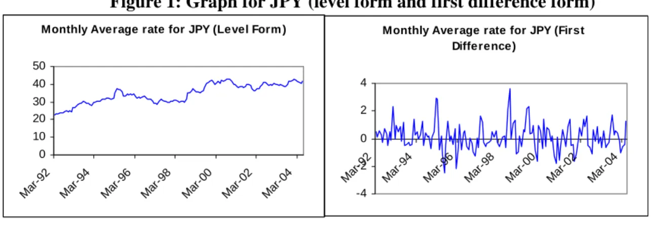
The Box-Jenkins methodology of building a model for this series begins with checking the series for stationarity. For this purpose series was plotted on the graph paper and also performed Unit root test (ADF9) and Correlogram analysis, all the three tests indicated that underlying series was not stationarity. But the first difference of the series was stationarity (See figure 1).
Figure 1: Graph for JPY (level form and first difference form)
9
In the ADF test of stationarity, if calculated value of tau-statistics is more than critical value at a given level of significance (in absolute terms), then one should reject the null hypothesis (H0 : δ= 0) or in other
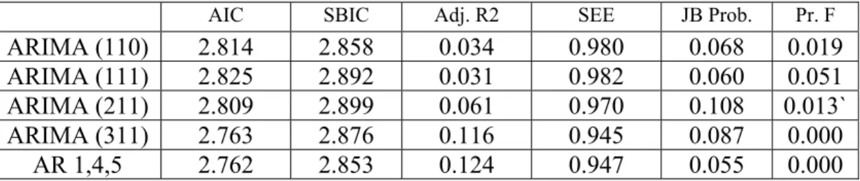
Correlogram of first difference series had significant ACF and PACF spikes at lag 1, which cut-off to zero immediately. Further series do not exhibit any significant spikes10 except at lag 4 and 5 for both ACF and PACF. It gives us a tentative idea to try with AR (1) or MA (1) or ARMA (1,1) and move further to add 4th and 5th order. After iterative process we find that ARIMA (3,1,1) and AR model with lag 1, 4 and 5 are two models better suited (see figure 2) to the given data on the basis of selected criteria (i.e. first error terms should be normally distributed, relatively small AIC or SBIC, Relatively small of SEE, Relatively high adjust R2 and overall fit of the model (F-statistics).
Figure 2: Comparison of Different Models for JPY
So these two models were selected for further analysis in terms of their ability to forecast accurately. Next table (figure 3) shows the comparison of the two models on the basis of various tests.
Figure 3: Comparison of Two Models for JPY
ARIMA (3,1,1) AR (1,4,5)
Mean Error (ME) 0.0385596 0.0094694
Mean Absolute Error (MAE) 0.5801059 0.5929072 Mean Squared Error (MSE) 0.5556437 0.477798 Mean Percentage Error (MPE) 0.08159 0.00528 Mean Absolute Percentage Error (MAPE) 1.42267 1.46296
Naïve11’s MAE 0.6432 0.6432
Naïve’s MAPE 1.58 1.58
Theil’s U statistics 1.0098105 0.9401678
As is cleared from the above table, AR model with lag 1, 4 and 5 more accurately forecast exchange rate of Japanese Yen (JPY) in terms of INR. So this model was finally selected.
10 Spike (or acf/pacf coefficient at a given lag is considered significant if absolute value of coefficient is
greater than 1.96 (1/√n ), where n is the number of observations.
11 Naïve’s Forecasting (NF1) approach attempts to check the accuracy of the model in relative form. It
involves two stages; first most recent observation is taken as forecast and MAE and MAPE for this forecast is calculated. In the second stage, MAE and MAPE so obtained is compared with the model under consideration and model is considered better if it gives less MAE and MAPE.
AIC SBIC Adj. R2 SEE JB Prob. Pr. F
ARIMA (110) 2.814 2.858 0.034 0.980 0.068 0.019
ARIMA (111) 2.825 2.892 0.031 0.982 0.060 0.051
ARIMA (211) 2.809 2.899 0.061 0.970 0.108 0.013`
ARIMA (311) 2.763 2.876 0.116 0.945 0.087 0.000
Here one more modification was required in the model, as first difference form of the series was used to build the model, which shows the changes in the exchange rate rather than the absolute exchange rate, so before forecasting the future values based on this model, it was integrated back to the level form.
AR model with lag 1, 4 and 5 was originally as:-
∆
y
t= c +
Ф
1∆
y
t-1+
Ф
2∆
y
t-4+
Ф
3∆
y
t-5So in level form it will be,
y
t= c + (
Ф
1+ 1) y
t-1-
Ф
1y
t-2+
Ф
2y
t-4+(
Ф
3-
Ф
2) y
t-5-
Ф
3y
t-6or, y
t= 0.133 + 1.162
y
t-1- 0.162y
t-2– 0.163y
t-4+0.0882y
t-5-0.251 y
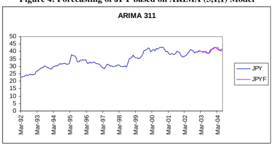
t-6 Figure 4: Forecasting of JPY based on ARIMA (3,1,1) ModelARIMA 311 0 5 10 15 20 25 30 35 40 45 50
Mar-92 Mar-93 Mar-94 Mar-95 Mar-96 Mar-97 Mar-98 Mar-99 Mar-00 Mar-01 Mar-02 Mar-03 Mar-04
JPY JPYF
Figure 5: Forecasting of JPY based on AR (1,4,5) Model
AR145 0 5 10 15 20 25 30 35 40 45 50
Mar-92 Mar-93 Mar-94 Mar-95 Mar-96 Mar-97 Mar-98 Mar-99 Mar-00 Mar-01 Mar-02 Mar-03 Mar-04
JPY JPYF
Monthly Average Rate for GBP (Level Form ) 0 20 40 60 80 100 M a r-9 2 M a r-9 4 M a r-9 6 M a r-9 8 M a r-0 0 M a r-0 2 M a r-0 4
Monthly Average rate for GBP (First Difference) -10 -5 0 5 M a r-9 2 M a r-9 4 M a r-9 6 M a r-9 8 M a r-0 0 M a r-0 2 M a r-0 4 Series1
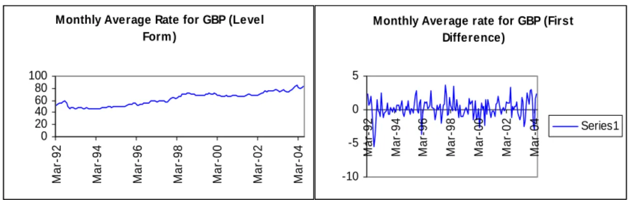
Indian Rupee (INR) versus Pound Sterling (GBP)
Graphical representation, Unit root test and Correlogram analysis showed that GBP series is not stationary (Figure 6) so first make it stationary by taking first difference of the series. Two more tests; Correlogram and Unit root test were performed to ensure that series had become stationary after taking first difference. Corrlogram of the difference series showed significant ACF at lag 1 which gradually decreased to zero and significant PACF at lag 1 and 2, which gave a tentative idea to proceed with either AR (2) or MA (1)
Figure 6: Graph for GBP (level form and first difference form)
or ARMA (2,1) process. But none of these models were giving normally distributed error terms (as was seen from very low p-values of J-B test). So we move further to test for higher order processes and ultimately found that ARIMA (4,1,4) and ARIMA (5,1,4) process were better suited for the given data (Figure 7).
Figure 7: Comparison of Different Models for GBP
AIC SBIC Adj. R2 SEE Pr. F JB Prob.
ARIMA (210) 3.438 3.505 0.026 1.33 0.068 0.000 ARIMA (011) 3.431 3.476 0.030 1.33 0.027 0.000 ARIMA (211) 3.451 3.541 0.021 1.33 0.129 0.000 ARIMA (414) 3.340 3.544 0.154 1.24 0.000 0.116 ARIMA (512) 3.314 3.496 0.175 1.23 0.000 0.012 ARIMA (514) 3.331 3.558 0.172 1.23 0.000 0.157 ARIMA (515) 3.376 3.626 0.143 1.25 0.001 0.107
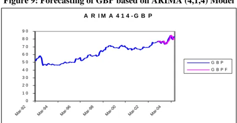
So these two models were selected for further analysis in terms of their ability to forecast accurately. Next table (figure 8) shows the comparison of the two models on the basis of various tests. As clear from this table, ARIMA (5,1,4) was better than ARIMA (4,1,4), so it was selected finally to forecast exchange rate of GBP in terms of INR.
∆yt = Ф1 ∆yt-1 + Ф2 ∆yt-2 + Ф3 ∆yt-3+ Ф4 ∆yt-4 + Ф5 ∆yt-5 + θ1 ut-1+ θ2 ut-2+ θ3 ut-3+ θ4 ut-4
Figure 8: Comparison of Two Models for GBP
ARIMA (4,1,4) ARIMA (5,1,4)
Mean Error (ME) 0.13273159 0.0966694
Mean Absolute Error (MAE) 1.66865209 1.5990937
Mean Squared Error (MSE) 3.54662157 3.4932872
Mean Percentage Error (MPE) 0.1374 0.0946
Mean Absolute Percentage Error (MAPE) 2.1229 2.0320
Naïve’s MAE 1.77111667 1.7711167
Naïve’s MAPE 2.251 2.251
Theil’s U statistics 0.9645881 0.9572996
So after integrating back at level form, it will be;
yt = 0.1845 + 0.5719 yt-1 + 0.6803 yt-2 – 0.4117 yt-3 – 0.3308 yt-4 + 0.3562 yt-5
+ 0.1346 yt-6 - 0.5304ut-1 – 0.2596ut-2 + 0.1475 ut-3 + 0.7463ut-4
Figure 9: Forecasting of GBP based on ARIMA (4,1,4) Model
A R I M A 4 1 4 - G B P 0 1 0 2 0 3 0 4 0 5 0 6 0 7 0 8 0 9 0
Mar-92 Mar-94 Mar-9 6
Mar-98 Mar-00 Mar-0 2
Mar-04
G B P G B P F
ARIMA 514 0 10 20 30 40 50 60 70 80 90
Mar-92 Mar-93 Mar-94 Mar-95 Mar-96 Mar-97 Mar-98 Mar-99 Mar-00 Mar-01 Mar-02 Mar-03 Mar-04
GBP GBPF
Indian Rupee versus EURO
The forecasting for exchange rate of Indian rupee in terms of Euro was not a straight-forward task, because Euro came into existence on January 1st, 1999 when eleven countries12 of European union (Belgian, Germany, Spain, France, Ireland, Italy, Luxemburg, Austria, Portugal, Finland and The Netherlands) decided to enter into a common currency regime. Thus, data for Euro are available for January 1999 onwards only and not prior to that. To avoid the data problem, we had a number of alternatives with us; first based on the irrevocable euro conversion rate13 we could generate the series of exchange rate for individual currencies1999 onwards. Second, based on the theoretical weightage14 given to each currency in the euro basket, we construct the quasi-euro rates prior to January 1999 and third, for period prior to January 1999 we could also use the exchange rate of ECU15 (ISO symbol XEU) as the proxy for euro. Each of these alternatives had their own limitations. While it was quite easy to generate the post 1999 series based on conversion rate, there was no practical use of such forecasting provided the fact that these individual currencies are no more used for international transactions. Technique of using theoretical weights seems to be appropriate, but non-availability of data for all the individual currencies prior to 1999 made it difficult to use this technique. Using European currency as proxy also had its own limitation, because being narrow based it does not properly represents euro.
12 List extended to 12 countries with the inclusion of Greece in January 2001.
13 On December 31 1998, midnight an irrevocable conversion rate for domestic currency with Euro (or
vice-versa too) and for the currencies of member states was fixed. Details can be obtained from
www.ecb.int
14 At the time of introduction of Euro, each member countries currency was given a weightage on two
aspects; narrow index and broad index. Deutsche Mark (around 35%) and French Franc (around 17.5%) were given the highest weights. Details can be obtained from Eurostat-Comext.
15 ECU was an artificial basket currency that was used by the member states of the EU as their internal
accounting unit. ECU was the precursor of new currency Euro, which was adopted on January 1, 1999. When Euro was introduced it replaced the ECU at par (1:1 ratio)
Monthly Average rate for Euro (DM converted series)- 1st difference series
0 20 40 60 80 M a r-9 2 M a r-9 4 M a r-9 6 M a r-9 8 M a r-0 0 M a r-0 2 M a r-0 4
Monthly Average rate for Euro (DM converted series)- 1st difference series
-4 -2 0 2 4 Mar -92 Mar -94 Mar -96 Mar -98 Mar -00 Mar -02 Mar -04
In this paper we made use of first and third techniques. In the first technique slight modification was done in the sense that instead of calculating the exchange rate for 1999 onwards, we took Deutsche Marks series prior to 1999 and convert it into euro series based on conversion rate. This series was not stationary, so we took first difference of the series to make it stationary (Figure 11).
Figure 11: Graph for Euro (level form and first difference form)
Figure 12: Comparison of Different Models for Euro (DM converted) AIC SBIC Adj. R2 SEE Pr. F JB Prob.
AR (1) 3.136 3.181 0.032 1.152 0.019 0.85 AR (2) 3.150 3.217 0.034 1.155 0.035 0.89 AR (3) 3.167 3.257 0.031 1.161 0.075 0.89 MA (1) 3.127 3.172 0.042 1.147 0.011 0.88 MA (2) 3.141 3.208 0.035 1.150 0.037 0.89 ARMA (111) 3.142 3.209 0.036 1.151 0.036 0.86 ARMA (211) 3.165 3.255 0.029 1.160 0.084 0.88
Correlogram of this series showed that it could be either AR (1) process or MA (1) process or ARMA (1,1,1) process. So we started with AR (1) process and checked other process also iteratively. By iterative process, we selected three processes AR (1), MA (1) and ARIMA (111) for further analysis (Figure 12).
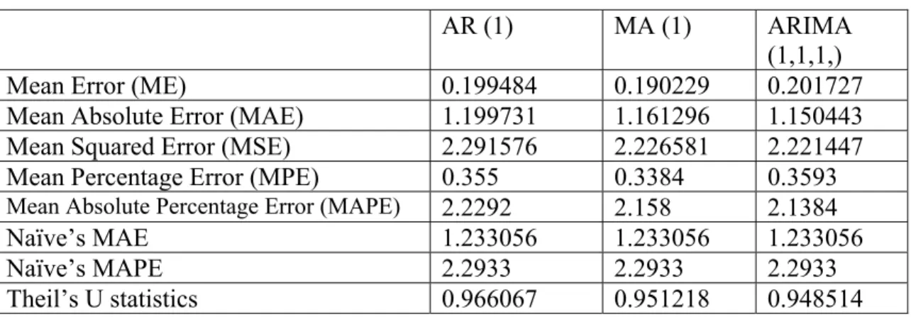
Figure 13: Comparison of Three Models for EURO (DM)
AR (1) MA (1) ARIMA
(1,1,1,)
Mean Error (ME) 0.199484 0.190229 0.201727
Mean Absolute Error (MAE) 1.199731 1.161296 1.150443 Mean Squared Error (MSE) 2.291576 2.226581 2.221447 Mean Percentage Error (MPE) 0.355 0.3384 0.3593
Mean Absolute Percentage Error (MAPE) 2.2292 2.158 2.1384
Naïve’s MAE 1.233056 1.233056 1.233056
Naïve’s MAPE 2.2933 2.2933 2.2933
ARIMA 111 0 10 20 30 40 50 60 70 Mar-9 2 Mar-9 3 Mar -94 Mar-9 5 Mar -96 Mar -97 Mar-9 8 Mar -99 Mar -00 Mar-0 1 Mar -02 Mar -03 Mar-0 4 DM DMF
A comparison of the three models on the basis of various statistical measures showed that ARIMA (1,1,1) model is more suitable for the given data. So this model was finally selected for forecasting exchange rate.
Figure 14: Forecasting of EURO (DM) based on ARIMA (1,1,1) Model
Our final model in level form is;
yt = 0.0979 + 0.8663yt-1 + 0.1336yt-2 +0.3638ut-1
ECU as Proxy for Euro
Next, we used ECU data as proxy for Euro prior to January 1999 and generated a series for that. As was expected from previous experience, original series was not stationary, but first difference transformation of the series was stationary. Correlogram of the first difference series indicated that series could be explained in terms of either AR (1) or MA (1) or ARIMA (1,1,1) process. By the iterative method and comparing various models, we finally selected ARIMA (1,1,1) for this series.
Our final model is;
y
t= 0.0877 + 0.7131y
t-1+ 0.2868y
t-2+0.5211u
t-1Figure 16: Comparison of Different Models for Euro (ECU Proxy Series)
AIC SBIC Adj. R2 SEE Pr. F JB Prob.
AR (1) 2.969 3.013 0.030 1.059 0.027 0.79 AR (2) 2.986 3.035 0.029 1.064 0.059 0.57 AR (3) 2.998 3.088 0.027 1.066 0.091 0.58 MA (1) 2.981 3.026 0.038 1.066 0.014 0.58 MA (2) 2.991 3.058 0.036 1.057 0.036 0.48 ARIMA (111) 2.969 3.036 0.037 1.055 0.035 0.40 ARIMA (211) 2.990 3.080 0.032 1.062 0.070 0.49 ARIMA (112) 2.984 3.074 0.029 1.059 0.080 0.40 ARIMA (212) 3.000 3.112 0.029 1.064 0.104 0.42
Figure 17: Comparison of Three Models for EURO (ECM)
AR (1) MA (1) ARIMA (1,1,1) Mean Error (ME) 0.215255 0.192947 0.21358033 Mean Absolute Error (MAE) 1.164208 1.120727 1.09463582 Mean Squared Error (MSE) 2.146903 2.062975 2.05424406 Mean Percentage Error (MPE) 0.385 0.345 0.383
Mean Absolute Percentage Error (MAPE) 2.1639 2.0832 2.036
Naïve’s MAE 1.217255 1.217255 1.21725459
Naïve’s MAPE 2.2639 2.2639 2.2639
Theil’s U statistics 0.962605 0.942828 0.93658921
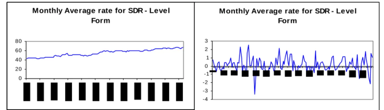
INR versus SDR
To forecast the exchange rate of SDR in terms of INR data from March 1993 onwards were taken. This adjustment in the data series was done to do away the impact of a drastic
Monthly Average for Euro (ECU Proxy)- Level Form 0 10 20 30 40 50 60 70
Monthly Average for Euro (ECU Proxy) 1st difference Form -4 -3 -2 -1 0 1 2 3 4
Monthly Average rate for SDR - Level Form 0 20 40 60 80
Monthly Average rate for SDR - Level Form -4 -3 -2 -1 0 1 2 3
correction that was done in February 199316. Series was not stationary, so first it was converted into stationary series by taking the fires difference of the series.
Figure 18: Graph for SDR level form and first difference form
Correlogram of first difference series had significant spikes at lag 1,2,5,14,20 and 21. That gave us a tentative idea to try for higher order ARIMA process also. We tried for various models and noted down the corresponding values of various selective criteria. Ultimately we short-listed three models; ARIMA (15,1,4), ARIMA (16,1,1) and AR (with lag 1,2,5,6,12-16) plus MA (1). When checked these three models for their forecasting accuracy, we found that ARIMA (15,1,4) is most suitable model to forecast exchange rate of SDR in terms of INR.
In the level form this model is;
y
t= 0.1828 + 1.1719y
t-1– 0.1682y
t-2+ 0.1100y
t-3+ 0.3413y
t-4– 0.1954y
t-5–
0.0899y
t-6- 0.0926y
t-7– 0.0622y
t-8+ 0.0173y
t-9+ 0.0401y
t-10– 0.024y
t-11+ 0.0801yt-12 - 0.0472yt-13 + 0.1774yt-14 – 0.2045yt-15 - 0.0541yt-16 -
0.1164ut-1 - 0.2848ut-2 - 0.2097ut-3 - 0.6490ut-4
Figure 19: Comparison of Different Models for SDR Exchange Rate AIC SBIC Adj. R2 SEE Pr. F JB Prob.
ARIMA (13,1,4) 2.526 2.983 0.109 0.791 0.050 0.06 ARIMA (13,1,5) 2.266 2.749 0.318 0.691 0.000 0.08 ARIMA (15,1,5) 2.427 2.968 0.227 0.744 0.002 0.13 ARIMA (15,1,4) 2.501 3.016 0.162 0.774 0.015 0.15 ARIMA (15,1,3) 2.509 2.998 0.149 0.780 0.019 0.05 ARIMA (16,1,3) 2.598 3.115 0.080 0.812 0.123 0.08 ARIMA (16,1,2) 2.568 3.060 0.100 0.803 0.073 0.11 ARIMA (16,1,1) 2.525 2.991 0.131 0.789 0.029 0.13 AR (1,2,5,6,9-16) MA (1) 2.464 2.827 0.156 0.778 0.007 0.32 AR (1,2,5,6,10-16) MA (1) 2.446 2.782 0.164 0.774 0.004 0.27
AR (1,2,5,6,11-16) MA (1) 2.441 2.752 0.161 0.775 0.004 0.29 AR (1,2,5,6,12-16) MA (1) 2.427 2.712 0.166 0.773 0.002 0.31
Figure 20: Comparison of Three Models for SDR
ARIMA (15,1,4) ARIMA (16,1,1) AR 1,2,5,6,12-16, MA (1)
Mean Error (ME) -0.20697 -0.17845798 -0.202962259
Mean Absolute Error (MAE) 0.775784 0.836958286 0.809161034 Mean Squared Error (MSE) 0.999335 1.059067493 1.019741363
Mean Percentage Error (MPE) 0.3289 0.2862 0.3234
Mean Absolute Percentage Error (MAPE) 1.1883 1.2814 1.24
Naïve’s MAE 0.882889 0.882888889 0.882888889
Naïve’s MAPE 1.3474 1.3474 1.3474
Theil’s U statistics 0.930576 0.9616225 0.945642195
Indian Rupee versus US Dollar
It was very hard to explain the behaviour of USD exchange rate data in terms of ARIMA process, even after exploring the possibility till 16th lag, so we had to conclude that ARIMA process is not suitable to explain the behaviour of this series and enable us to forecast the exchange rate of USD in terms of Indian rupee.
Figure 21: Forecasting of SDR based on ARIMA (15,1,4) Model
ARIMA (15,1,4) 0 10 20 30 40 50 60 70 80 Mar -93 Mar -94 Mar -95 Mar -96 Mar -97 Mar -98 Mar -99 Mar -00 Mar -01 Mar -02 Mar -03 Mar -04 SDR SDRF
Conclusion
Based on the result of this paper, we can conclude that exchange rate do not exhibit a random walk and it is quite possible to build a model for it, although slightly difficult. Again ARIMA methodology produces superior results than only AR process or MA process. We are able to build a model for all the currencies under our study, except for US Dollar, which shows the relatively efficiency of the currency market for dollar.
Further Scope
In recent time a number of newer and more sophisticated techniques have been developed to build univariate models for the purpose of forecasting. To name a few, Bayesian Vector Auto-regression (BVAR), Bayesian Vector Error Correction Model (BVECM), exponential smooth transition autoregressive (ESTAR) model, Bootstrap technique, PC ARIMA, ARCH models, a full family of GARCH models and various other non-linear models, so one can further work on the same paper using these methodology and try to find out if these models have the ability to produce more accurate forecast.
References
• An Sing Chen and Mark T. Leun, “ A Bayesian vector error correction model for forecasting exchange rates”, Computers & Computers & Operations Research 30 (2003) 887–900.
• An Sing Chen and Mark T. Leun, “ Regression neural network for error correction in foreign exchange forecasting and trading”, Computers & Computers & Operations Research 31 (2004) 1049-1068.
• Cao R., García Jurado I., Gonzalez Manteiga W., Prada Sanchez J.M. and Febrero-Bande M., “Predicting using Box-Jenkins, nonparametric and bootstrap techniques” Technometrics 37 (1995) 303-310.
• European Monetary Institute’s report on progress towards convergence 1996.
• “Exchange Rate Forecasting; techniques and applications” by Imad A. Moosa, Macmillan Business, London 2000.
• Harald Reinton and Steven Ongena, “ Out-of-sample forecasting performance of single equation monetory exchange rate models in Norwegian currency market”, Applied Financial Economics, 1999, 9, 545-550.
• Jeffrey M. Wrase, “The Euro and the European Central Bank”, Business Review, November/December 1999.
• Lindsay I. Hogan, “A comparision of alternative exchange rate forecasting models”, Bureau of agricultural Economics, Canberra ACT 2601.
• Lutz Lillian and Mark P. Taylor, “Why it is so difficult to beat random walk forecast of exchange rates?”, Journal of International Economics 60 (2003) 85-107.
• Mary E. Gerlow and Scott H. Irwin, “ The performance of exchange rate forecasting models: an economic evaluation”, Applied Economics, 199123, 133-142.
• Pilar Olave and Jesus A. Miguel, “Bootstrap Method in Exchange Rate Forecasting”, University of Zaragoza, Spain.
Books
• John Faust, John H. Rogers, Jonathan H. Wright “Exchange rate forecasting: the errors we’ve really made”, Journal of International Economics 60 (2003) 35-59
• International Financial Management by prakash G. Apte , 3rd edition, Tata Mcgraw hill publication Pg. 325-330
• Introductory econometrics for finance by Chris Brooks, Ist edition, Cambridge University press, Pg. 229-301.