Load frequency control of large scale power system using quasi-oppositional grey wolf optimization algorithm

Full Length Article

Load frequency control of large scale power system using

quasi-oppositional grey wolf optimization algorithm

Dipayan Guha

, Provas Kumar Roy

, Subrata Banerjee

a_{Department of Electrical Engineering, Dr. B.C.Roy Engineering College, Durgapur, West Bengal, India} b

Department of Electrical Engineering, Jalpaiguri Government Engineering College, Jalpaiguri, West Bengal, India c

Department of Electrical Engineering, National Institute of Technology, Durgapur, West Bengal, India

a r t i c l e i n f o

Received 2 August 2015 Revised 14 May 2016 Accepted 6 July 2016 Available online 18 July 2016 Keywords:

Load frequency control Grey wolf optimization Oppositional based learning Quasi-oppositional based learning Sensitivity analysis

a b s t r a c t

This article presents a newly developed, novel and efficient optimization technique called quasi-oppositional grey wolf optimization algorithm (QOGWO) for the first time to solve load frequency control problem (LFC) of a power system. Grey wolf optimization (GWO) is a recently developed meta-heuristic optimization technique based on the effect of leadership hierarchy and hunting mechanism of wolves in nature. Two widely employed test systems; viz. two-area hydro-thermal and four-area hydro-thermal power plant, are considered to establish the effectiveness of the proposed QOGWO algorithm. Optimal proportional-integral-derivative controller (PID) is designed for each area separately using proposed algorithm employing integral time absolute error (ITAE) based fitness function. The validity of proposed QOGWO method is tangibly verified by comparing its simulation results with those of GWO and other approaches available in the literature. Time domain simulation results confirm the potentiality and effi-cacy of the proposed QOGWO method over other intelligent methods like fuzzy logic, artificial neural net-work (ANN) and adaptive neuro-fuzzy interface system (ANFIS) controller. Finally, sensitivity analysis is performed to show the robustness of the designed controller under different uncertainty conditions. Ó2016 Karabuk University. Publishing services by Elsevier B.V. This is an open access article under the CC

BY-NC-ND license (http://creativecommons.org/licenses/by-nc-nd/4.0/).

1. Introduction

Stable operation of power system requires matching between total generation with total load demand and with accompanying system losses. Due to rising and falling of load demand, the real and reactive power balance is disturbed, resulting deviation of sys-tem frequency and tie-line interchange power from their sched-uled value. High deviation of system frequency may lead to system collapse. This encourages designing of an accurate, effective and fast controller in power system called load frequency con-troller (LFC) to maintain system parameters, i.e. area frequency, and tie-line interchange power, at their predefined values. LFC is one of the most profitable ancillary services to be maintained for

the smooth and secure operation of power system[1,2]. The

objec-tive of LFC is to diminish transient deviations of area frequency and tie-line interchange power and to confirm their steady state errors to be zeros. In today’s scenario, LFC is one of the most prominent issues for supplying sufficient and reliable electric power with

good quality to the customers and is becoming much more signif-icant in accordance with increasing size of power system unit, changing of structure and drastic change in load demand. The main

functions of load frequency controller are as follows[3]:

1. The steady state frequency error following a step load change should vanish. The transient frequency and time errors should be small.

2. The static change in tie-line power following a step load pertur-bation in any area should be zero, provided each area can accommodate its own load change.

3. Any area in need of power during any emergency should assist from others.

During the last few decades, various control strategies based on

classical controllers[4–10], adaptive controller[11], robust

con-troller [12], intelligent controllers including neural network

[1,2,13], fuzzy logic[14–16], H1controller [17], fractional order

controller [18], internal model control [19], hybrid neuro-fuzzy

controller[20]etc. have been demonstrated to maintain the

sys-tem frequency and tie-line interchange power at their nominal

value under normal and disturbed conditions. In[6], several

classi-cal controllers’ structure like integral (I), proportional integral (PI),

http://dx.doi.org/10.1016/j.jestch.2016.07.004

2215-0986/Ó2016 Karabuk University. Publishing services by Elsevier B.V.

This is an open access article under the CC BY-NC-ND license (http://creativecommons.org/licenses/by-nc-nd/4.0/).

⇑ Corresponding author.

E-mail address:[email protected](D. Guha). Peer review under responsibility of Karabuk University.

Contents lists available atScienceDirect

Engineering Science and Technology,

an International Journal

integral derivative (ID), proportional integral derivative (PID) and integral double derivative (IDD) were implemented and their com-parative performances for the LFC system have been presented.

Oysal [11] proposed dynamic neural network (DNN) model for

adaptive LFC design in power systems. In [18], authors have

designed an optimal fractional order PI and PID controller to improve the dynamic stability of automatic generation control (AGC) system employing integral time absolute error (ITAE) based performance index. Internal model control scheme with model

order reduction technique was elaborated in [19]. A hybrid

neuro-fuzzy controller was suggested in[20]as a supplementary

controller to solve LFC problem in a restructured environment of the power system. Although the aforesaid methods improve the dynamic stability of power system, they require extensive compu-tation. Moreover, high order, complexity, a requirement of large training data set, defuzzification operations, inference mechanism etc. makes the controller inapplicable for the real-time implemen-tation. Recently, the effect of redox flow batteries in LFC of

multi-area power system has been investigated in[21].

It is perceived in the power system that parameter values in the various power generating units, viz. governors, turbines, genera-tors etc., are endlessly varying w.r.t time subject to system and power flow condition. Thus, the controller parameters design at normal operation may not able to give satisfactory performance under external disturbed and/or parameter uncertainty condition. To ensure robustness and to preserve the system stability, various populations based meta-heuristic optimization techniques such as

particle swarm optimization (PSO) [22], genetic algorithm (GA)

[23], biogeography-based optimization (BBO) [24,25], krill herd

algorithm (KHA)[26], teaching learning based optimization (TLBO)

[27,28], bacteria foraging optimization (BFOA) [7], gravitational

search algorithm (GSA) [29], hybrid PSO-pattern search

(hPSO-PS) algorithm [30], hybrid FA-PS [31], Tabu search algorithm

(TSA)[32], quasi-oppositional harmony search algorithm (QOHSA)

[33,34], BAT algorithm[35], backtracking search algorithm (BSA)

[36], were proposed in the literature. Padhan et al. [4] have

designed an optimal LFC by employing firefly algorithm (FA) and showed its superiority over other similar optimization techniques.

Nanda et al.[6]demonstrated that BFOA has better tuning ability

than GA and Zeigler–Nichols (ZN) based controller for an intercon-nected power system. An improved PSO algorithm was elaborated

in[8]for a nonlinear multi-area hybrid power system comprising

thermal-hydro-gas power plant. In[9], lozi map chaotic

optimiza-tion algorithm was proposed for the design of PID-controller to

solve LFC problem in power system. In [24,25], BBO algorithm

was successfully designed and applied to a nonlinear intercon-nected power system and showed its superiority over other opti-mization methods. However, the performance of BBO is highly determined by the maximum emigration and immigration rate, mutation probability, the step size of integration, habitat

modifica-tion probability etc. Guha et al.[26]have offered KHA for

multi-area power system considering flexible alternating current trans-mission system (FACTS) controller. A tabu search algorithm (TSA) for finding the optimal solution of LFC problem was reported in

[32]. The main advantage of TSA is its ability to escape from local

solution and fast convergence speed. However, conventional TSA might have the problem of reaching a global optimum solution in an equitable time when the initial solution is far away from

the region where the global solution exists. Shiva et al.[33]have

addressed an improved harmony search algorithm with the theory of quasi-oppositional based learning (Q-OBL) so as to tune the LFC parameters under the deregulated environment. In the design of HAS, determination of harmony memory consideration rate, pitch adjusting rate and a number of improvisation are obligatory.

Abd-Elazim et al.[35]have proposed bat algorithm based optimal

PI-controller for the effective solution of LFC problem and

established the supremacy of bat algorithm over simulated anneal-ing in tunanneal-ing PI-controller usanneal-ing different performance indices. Guha in his most recent endeavor has explained the solution of

LFC problem using BSA[36]. Shabani et al. [37] have employed

an imperialist competitive algorithm (ICA) to optimize the PID-controller gains in a multi-area multi-unit power system. Simu-lated annealing based optimal controller for the control of system frequency and terminal voltage of an interconnected multi-area

multi-source power system is discussed in[38]. In [39], the use

and effectiveness of interline power flow controller (IPFC) in LFC area have been investigated. Although the aforementioned meth-ods give an optimal solution of LFC problem leaving behind some deficiencies which are further corrected by the researchers. The main drawback is the slow convergence towards the optimal solu-tion and more or less all aforesaid techniques depends on the proper initialization of input parameters. Additionally, the algo-rithms demand proper tuning of some of their own input control parameters. For example, GA involves the determination of algorithm-specific parameters such as crossover rate and mutation rate. PSO has its own parameters like inertia weight, social and cognitive parameters. If the parameters are not properly defined, the algorithm may easily trap into local optimum solution. Thus exploring new optimization technique is still prevailing to enhance the relative stability of power system, especially, by the design of an optimal controller.

Grey wolf optimization (GWO)[40]is a new optimization

tech-nique proposed by Mirjalili et al. in 2014 and hardly being used in power system to solve LFC problem. However, the literature review reveals that the proposed GWO algorithm has been successfully applied to different areas of power system for betterment of the

existing results[41–45]. The GWO algorithm simulates the

leader-ship hierarchy and hunting mechanism of grey wolves in nature. Unlike other optimization technique, GWO only requires defining of population size and a maximum number of iteration for its func-tionality. In this article, the quasi-oppositional based learning (Q-OBL) theory is integrated into conventional GWO to accelerate its convergence rate and to minimize the computational intricacy. The proposed approach is applied for the first time to solve LFC problem in an interconnected power system.

The main contribution of this paper to:

(i) demonstrate the effectiveness of proposed scheme, initially two-area hydro-thermal power plant is investigated and then the study is forwarded to a more complex and realistic test system considering the four-area hydrothermal system. (ii) propose an optimal design of PID-controller for the effective

and simple solution of load frequency control problem. (iii) frame a novel optimization scheme utilizing Q-OBL theory

with original GWO algorithm.

(iv) add some degree of complexity, possible inherent power system nonlinearities like governor dead-band, time-delay, and generation rate constraint are integrated into the sys-tem modeling.

(v) demonstrate the advantage of proposed algorithm, dynamic responses of the concerned power system are compared to those yielded by other existing results available in the liter-ature by transient analysis method.

(vi) discuss the dynamic behavior of the concerned test system by applying a realistic load pattern and aggregated load in all the areas for the sake of its robustness analysis. (vii) show the robustness of proposed technique, sensitivity

anal-ysis is performed over a wide variation of system parameters and loading conditions.

The rest of the paper is organized as follows: The dynamic

problem description. A brief outline of GWO algorithm is

elabo-rated in Section3 followed by its algorithmic steps applied to

LFC system. The theory of Q-OBL is given in Section4 followed

by algorithmic steps of proposed QOGWO algorithm for the

solu-tion of LFC problem in Secsolu-tion5. Section6highlights the

simula-tion results and comparative analysis of concerned power

system. Finally, Section7concludes the present analysis.

2. Problem formulation

A dynamic model of interconnected test system should first develop in order to implement an appropriate control scheme for enhancing the dynamic stability of the power system. Initially, a two-area hydro-thermal power system is designed and its dynamic responses are investigated and later the study is forwarded to a four-area hydro-thermal power system. QOGWO algorithm is used to design optimal PID-controller for each area employing ITAE based fitness function. 1% step load perturbation in area-1 is con-sidered to demonstrate the dynamic stability of concerned power

system.Fig. 1shows the transfer function model of the test system.

The nominal values of system parameters are taken from[1]and

presented inTable 1A. Fig. 1 Ri represents the speed regulation

constant of governor,Bi is the frequency bias constant,Tsg is the

hydraulic time constant,Ttis the turbine time constant,Tr is the

reheat time constant,Kris the reheat gain,Kpsis the control area

gain,Tpsis the control area time constant,Twis the water starting

time of hydro-turbine,KD;KP;KI are the electric governor

deriva-tive, proportional and integral gains, respectively,Df1andDf2are

the frequency deviations in area-1 and area-2 respectively, DPtie

is the tie-line power deviation andDPDis the incremental change

in system loading condition. Inputs to the PID-controllers are the area control error (ACE) of respective areas and controlled inputs

ðu1;u2Þto the plant with PID-controller structure are defined as

follows: ACE1¼B

D

D

D

D

ACE is treated as controlled output of LFC system, which is used to identify any mismatch between power generation and load demands. In an optimal control system, the selection of objective function is done either by (i) taking few points of the time

response, or (ii) by taking the entire time response, i.e. integral

Fig. 1.Transfer function model of two-area hydro-thermal power system (test system-1)[1].

Table 1A

Nominal values of system parameters.

Parameter Values Parameter Values Parameter Values Parameter Values

Test System-1[1] f 60 Hz Tti 0.3 s B1¼B2 0.425 p.u MW/Hz Tr 10 s Pr1¼Pr2 2000 MW Tgi 0.08 s Kp1¼Kp2 120 Kr 0.5 R1¼R2 2.4 Hz/p.u MW Tpi 20 s 2pT12 0.545 Tw 1 s KP 1 KI 5 KD 4 a12 1 Test system-2[13] f 50 Hz Tti 0.3 s Bi 0.425 p.u MW/Hz Tr 10 s Pri 2000 MW Tgi 0.08 s Kpi 120 Kr 0.5 Ri 2.4 Hz/p.u MW Tpi 20 s 2pTi;j 0.545 Tw 1 s KP 1 KI 5 KD 4 a12 1

criterion. Integral criterion is the most commonly used mance index in optimal control theory. The commonly used perfor-mance indices based on integral criterions are the integral square error (ISE), integral absolute error (IAE), integral time multiplies of square error (ITSE) and ITAE.

ISE is a measure of system performances formed by integrating the square error over fixed interval of time. It exhibits smaller overshoot but albeit large settling time. IAE is error taken absolute and added over time. It is often used where digital simulation of a system is employed. However, it is irrelevant to real-time analyti-cal work, since the determination of the absolute value of error in analytic form is somewhat difficult. It produces a slower system response. ITAE and ITSE have an additional time multiplier of the error function, which highlight long duration errors and gives fas-ter time response compared to ISE and IAE. ITAE integrates the absolute error multiplied by the time over time. What this does is to weight errors which exist after a long time much more heavily than those at the beginning of the response. ITAE based tuning makes the system to settle down much faster than the other said tuning methods. ITAE criterion also provides minimum peak over-shoot. On the other hand, ITSE criterion based controller offers large controller output for the sudden change in reference value, which is not wanted from the controller design point of view.

Thus, ITAE based objective function is considered to tune the controller parameters using QOGWO algorithm. The fitness

func-tion or objective funcfunc-tion (J) is defined as:

J¼ Z Tfinal

0

t jð½

D

D

D

whereTfinal is the final simulation time.

The problem constraints are the controller parameter bounds; hence, optimal design of LFC problem can be formulated as follows:

MinimizeJ:

Subjected to:KP;min6KP6KP;max;KI;min6KI6KI;max;KD;min

6KD6KD;max ð4Þ

whereKPID;minandKPID;maxare the minimum and maximum value of

PID-controller parameters respectively, which are selected between

[0, 2][36,49]. The typical block diagram of gain scheduling method

with the proposed QOGWO algorithm is shown inFig. 2.

3. Grey wolf optimization

In the recent times, meta-heuristic optimization techniques like GA, GSA, ACO, PSO etc. are becoming more famous in the area of swarm intelligence (SI). Said techniques are not only successfully applied to the power system domain but it spreads its wings to other research areas. Mainly there are four basic reasons behind the popularity of these algorithms; these are (i) simplicity, (ii) flex-ibility, (iii) derivative-free mechanism, and (iv) local optima

avoid-ance[40]. Nearly all the conventional optimization methods are (i)

nature inspired, (ii) randomly initialized, and (iii) they have several input parameters those need to be fitted to the problem in hand. In addition to this, they are also suffering from the long computa-tional time, poor convergence rate, large dimension, no guarantee to give the global optimum solution, growing to need more com-puter resources. According to ‘No-Free-Lunch’ theorem, there is no meta-heuristic optimization method well suited for all opti-mization problems and there is always a room for improvement. Having knowledge of the aforesaid discussion, a novel nature-inspired optimization technique called grey wolf optimization (GWO) inspired by social hierarchy and hunting behavior of grey wolves is proposed for solving LFC problem. The advantages of GWO algorithm are: (i) it is free from the initialization of input parameters, (ii) straightforward and free from computational com-plexity, (iii) ease of transformation of such concept to the program-ming language, and (iv) ease of understanding. In this section, first, the encouragement of GWO technique is discussed and thereafter the mathematical modeling of GWO algorithm is elaborated.

3.1. Encouragement of GWO

Grey wolf, also known as the timber wolf or western wolf, belongs to Canidae family and its scientific name is Canis Lupus. Grey wolfs are normally considered as apex predators (at the top of the food chain) and popularly available in remote areas of North America, Eurasia and northern, eastern and western Africa. The -grey wolf optimization (GWO) algorithm is introduced by Mirjalili

et al. in 2014[40]which simply mimic the leadership hierarchy

and hunting mechanism of grey wolves in nature. Grey wolfs mostly prefer to live in the pack (5–12 on average). Four types of

grey wolves such as alpha (

a

are employed for simulating the leadership hierarchy. In addition to that, three main steps of hunting like searching for prey, encir-cling prey and attacking prey are implemented to perform optimization.

Grey wolves present at the top of the hierarchy are called as alpha category wolves and they are the leader of the whole pack. This category of wolves may be male or female and has decision-making power about hunting, sleeping place, time to wake etc. Their decisions are directed to the pack. However, some kind of democratic behavior is also observed for which they follow other wolves in the pack. Interestingly, alpha is not necessarily the stron-gest member in the hierarchy, it only manages the pack.

In the second level of the hierarchy, the grey wolves are named as beta category wolves and they are subordinate to the alpha cat-egory. They help alphas in decision-making and other movements of the pack. The betas are probably the best candidate of alpha in case one of the alpha wolves passes away or become very old. It plays the role of an advisor to alphas and discipliner in the pack.

The lowest stage of the hierarchy is occupied by the omega types of wolves. They are basically used as a scapegoat and always follow the decision made by other dominant wolves. It is noted Fig. 2.Control strategy for gain scheduling of controller settings using QOGWO

that omega types of wolves are not so much important in the pack, but the whole pack may face internal fighting in case of losing the omega. Omegas are always maintaining the dominant structure in the hierarchy and sometimes they can use as babysitters in the pack.

The wolves which don’t come under alpha, beta and omega cat-egory are grouped under delta catcat-egory. Delta types of wolves always follow the alphas and betas but dominate omegas. Five basic things come under this hierarchy such as (i) scouts, (ii) sen-tinels, (iii) elders, (iv) hunters and (v) caretakers. Scouts are responsible for watching the boundaries and alert the pack in case of any danger. Sentinels protect and confirm the safety of the pack. Elders are the experienced wolves (alphas or betas) and their expe-riences are used to attack prey or any target elements. Hunters help alphas or betas when hunting prey and providing food for the pack. Finally, caretakers are responsible for caring the feeble, sick and injured wolves.

The main steps of grey wolf hunting are as follows[40]:

(i). Tracking, chasing and approaching the prey

(ii). Pursuing, encircling and harassing the prey until it stops moving

(iii). Attack towards the prey

3.2. Mathematical modeling of GWO

In this section, the social hierarchy of wolves, tracking, encir-cling and attacking prey are discussed followed by the mathemat-ical modeling of GWO algorithm.

3.2.1. Social hierarchy

For modeling of the social behavior of the grey wolf, alpha is considered to be the fittest solution followed by beta and delta, respectively, and the rest of the solutions are grouped under omega. In GWO, the hunting (optimization) process is guided by alpha, beta and delta, whereas omega always follows these three wolves.

3.2.2. Encircling

To model the encircling behavior of grey wolves around the

prey, following equations are considered[40].

~

D¼ j~C:~xpðtÞ ~xðtÞj ð5Þ

~xðtþ1Þ ¼~xpðtÞ ~A~D ð6Þ

where,tis the current iteration,~xpðtÞdenotes the current position of

the victim, and the coefficient vectors~Aand~Care computed using

(7) and (8), respectively.

~_{A¼2~a~r1~a ð7Þ}

~_{C¼2~r2 ð8Þ}

where,~r1and~r2 are two random vectors between [0, 1] and the

component of~ais linearly decreasing from 2 to 0 over each course

of the iteration.

3.2.3. Hunting

In hunting phase which is basically guided by the alphas, the positions of the grey wolves are updated. Though alphas are the main agents in hunting phase, still occasionally betas and deltas also participate in the hunting process. So far we have the candi-date solutions of grey wolves in terms of alphas, betas and deltas but we don’t know the exact or optimum position of prey. To find the optimum positions, three best solutions (obtained so far) in terms of alpha, beta and delta are saved and remaining solutions

including omega compete. Following formulas are used to update

the wolf positions around the prey[40].

~ Da¼ j~C1~XaX~j; ~Db¼ j~C2~Xb~Xj; ~Dd¼ j~C3~Xd~Xj ð9Þ ~ X1¼~Xa~A1ðD~aÞ; ~X2¼~Xb~A2ð~DbÞ; ~X3¼~Xd~A3ð~DdÞ ð10Þ ~ Xðtþ1Þ ¼~X1þ~X2þ~X3 3 ð11Þ

It would be observed that final position is random in nature within the circle which is completely defined by the alpha, beta and delta in the search space, whereas other wolves update their position by estimating the prey position.

3.2.4. Attacking prey (exploitation)

Exploitation refers to local search capability around the promis-ing regions obtained in the exploration phase. In the above sec-tions, it is discussed that how the grey wolves finish the hunt by attacking prey when it stops moving. In order to mathematically express the model approaching the prey, two parameters, as

described below are considered.~ais linearly decreasing from 2 to

0 and fluctuations of~Ais also decreased with~a. In other words~A

is a random value between ½a;a: When random value of~A is

between [1, 1], the next position of search agent can be any

posi-tion between current posiposi-tion and prey posiposi-tion.

3.2.5. Search for prey (exploration)

The exploration phase refers to the course of investigating the promising area of the search space as broadly as possible. Opti-mum search in grey wolf algorithm is based on the positions of alpha, beta and delta. They diverge from each other when they search for prey and converge during attacking the prey.

Mathemat-ically, when random value of~Ais greater than 1 or less than -1,

search agent diverges to prey. This emphasizes exploration behav-ior in GWO algorithm. One more variable in GWO technique helps

exploration process is~C. The random value of~C varies between

[0,2], as evident from(8), which affects the prey of defining the

dis-tance as in(5). Thus, GWO shows more random behavior

through-out the optimization and favoring exploration and local optima avoidance.

Finally, the algorithmic steps of GWO may be summarized as follows:

(a) The search process is started with random initialization of candidate solutions (wolves) in the search space.

(b) Alpha, beta and delta wolves are estimated based on the position of prey.

(c) To find the optimum location of prey, each wolf updates its position.

(d) A control parameter~alinearly decreases from 2 to 0 for

bet-ter exploitation and exploration of candidate solutions.

(e) Candidate solutions tend to diverge when~A>1 and to

con-verge when~A<1 and at the end GWO gives the optimum

solution.

The general flowchart of GWO algorithm is shown inFig. 3and

for more details about the GWO algorithm; readers are referring to

[40].

4. Quasi-oppositional based learning (Q-OBL)

Oppositional based learning (OBL) developed by Tizhoosh[46]

and to accelerate the convergence rate of different optimization techniques in the field of artificial intelligence. OBL considered cur-rent population and its opposite population at the same time to generate better candidate solution. In OBL, the opposite number is generated at the mirror point of the solution from the center of the defined search space. In the recent times, OBL is established to increase the convergence rate of innumerable optimization

methods like GSA[47], ant colony optimization (ACO)[48], BBO

[49], TLBO[50], harmony search algorithm (HSA)[31,32]etc. The

researchers in the field of optimization claim that an opposite number is better than a pseudo random number for finding the global solution.

The opposite number and opposite point, as used in OBL, has straightforward definition as follows:

Let, an initial populationðyO_{Þbe a real number in an interval}

½a_;b, i.e.yO_{2 ½a;b, whereaandbare two extreme points of the}

search space and its opposite populationðyOP_{Þis mathematically}

defined by (12)in 1-dimensional search space. The definition of

the opposite population can easily extend tod-dimensionalsearch

space and it is defined by(13).

yOP_¼aþbyO _ð12Þ

yOP

i ¼aiþbiyO ð13Þ

whereyi2 ½ai;bi;i¼1;2; ;d:

It is evident from Simon et al.[51]that quasi-oppositional

ber is usually closer to the optimal solution than an opposite num-ber. The quasi-oppositional number is defined at the center of the

search space and opposite number. Ford-dimensionalsearch space,

quasi-oppositional number is expressed as follows: yQOP i ¼rand aiþbi 2 ;y OP i i¼1;2; ;d ð14Þ

The evolutionary process may be forced to skip or jump

based on jumping rate ðJrÞ to a new candidate solution which

is fitter than the current one. After generating new population

based on ðJrÞ, the quasi-opposite population is calculated and

the best population gets sorted from the union of current and quasi-opposite population based on candidate solution. In the present study, authors define a time-varying jumping rate as

shown in(15). Jr¼ Jr;maxJr;min Jr;maxJr;min NFCmaxNFC NFCmax ð15Þ

whereJ_r;minandJr;maxare the minimum and the maximum value of

jumping rate, respectively, NFCmax is the maximum number of

function call,NFCis the maximum number of function call at the current iteration. In the present study, authors considered the min-imum and the maxmin-imum value of jumping rate are 0 and 0.3, respectively.

5. Algorithmic steps of QOGWO applied to LFC problem

Step 1 Initialize the input parameters of original GWO

algo-rithm, i.e. population sizeðnpÞ, the number of control

variablesðdimÞ, the minimum and the maximum

jump-ing rate.

Step 2 Initial populations, i.e., search agents or grey wolves

(LFC parameters Kp;Ki;Kd) are randomly generated

within the defined solution space and calculate fitness

function using(3).

Step 3 Generate quasi-opposite population at the center of the

search space and opposite population using(14).

Calcu-late fitness function using(3).

Step 4 SelectNp (population size) fittest population from the

union of the current and quasi-opposite population. Step 5 Filter out some elite solutions based on fitness value.

Step 6 Define

_a

calculate fitness value.

Step 7 Update the positions of

a

the following pseudo code:

for i_¼1_:Np if fitness<alpha

alphaupdatefitness end

if fitness>alpha&&fitness<beta betaupdatefitness

end

if fitness>alpha&&fitness>beta&&fitness<delta deltaupdatefitness

end end

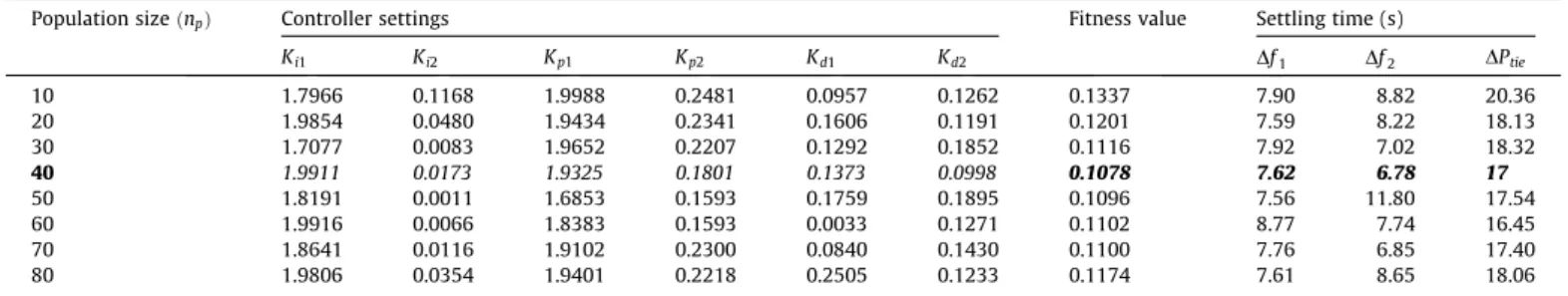
Table 1B

Comparative transient performance of test system-1 with different number of grey wolves employing QOGWO algorithm.

Population sizeðnpÞ Controller settings Fitness value Settling time (s)

Ki1 Ki2 Kp1 Kp2 Kd1 Kd2 Df1 Df2 DPtie 10 1.7966 0.1168 1.9988 0.2481 0.0957 0.1262 0.1337 7.90 8.82 20.36 20 1.9854 0.0480 1.9434 0.2341 0.1606 0.1191 0.1201 7.59 8.22 18.13 30 1.7077 0.0083 1.9652 0.2207 0.1292 0.1852 0.1116 7.92 7.02 18.32 40 1.9911 0.0173 1.9325 0.1801 0.1373 0.0998 0.1078 7.62 6.78 17 50 1.8191 0.0011 1.6853 0.1593 0.1759 0.1895 0.1096 7.56 11.80 17.54 60 1.9916 0.0066 1.8383 0.1593 0.0033 0.1271 0.1102 8.77 7.74 16.45 70 1.8641 0.0116 1.9102 0.2300 0.0840 0.1430 0.1100 7.76 6.85 17.40 80 1.9806 0.0354 1.9401 0.2218 0.2505 0.1233 0.1174 7.61 8.65 18.06

Bold shows the best results.

10 20 30 40 50 0.105 0.11 0.115 0.12 0.125 0.13 0.135 0.14 number of generation fi tn e s s va lu e (a) QOGWO GWO 10 20 30 40 50 0.024 0.026 0.028 0.03 0.032 0.034 0.036 0.038 0.04 0.042 number of generation fitn e ss va lu e (b) QOGWO GWO

Fig. 4.Convergence characteristics of proposed algorithm, (a) test system-1, (b) test system-2.

Table 2

Optimal value of controller gains, ITAE value and settling time of system oscillations of test system-1.

Evolutionary algorithm PID-controller gains ITAE value Settling time (s)

Ki1 Ki2 Kp1 Kp2 Kd1 Kd2 Df1 Df2 DPtie

GWO 1.8498 0.0418 1.9352 0.2916 0.2091 0.1863 0.1216 7.64 8.98 18.98

QOGWO 1.9911 0.0173 1.9325 0.1801 0.1373 0.0998 0.1078 7.62 6.78 17

0 5 10 15 -20 -15 -10 -5 0 5x 10 -3 time in sec fr equency devi ati o n i n H z (a) GWO QOGWO PID [1] Fuzzy [1] ANN [1]

0

2

4

6

8

10

12

14

-20

-15

-10

-5

0

x 10

time in sec

frequency

d

ev

iat

ion

in

H

z

(b)

GWO

QOGWO

PID [1]

Fuzzy [1]

ANN [1]

0

5

10

15

-3

-2

-1

0

1

x 10

time in sec

ti

e-l

in

e pow

er devi

ati

o

n i

n

p.

u.

(c)

GWO

QOGWO

PID [1]

Fuzzy [1]

ANN [1]

Fig. 5.Transient performance of test system-1 after 1% SLP in area-1 (a) change in frequency of area-1, (b) change in frequency of area-2, and (c) change in tie-line power.

0 5 10 15 -10 -8 -6 -4 -2 0 2 4x 10 -3 time in sec A rea co nt rol error (a) area-1 area-2 0 5 10 15 20 -9 -8 -7 -6 -5 -4 -3 -2 -1 0 1x 10 -3 time in sec A rea co nt rol error (b) area-1 area-2 area-3 area-4

Step 8 Defining two random numbersr1;r2between [0, 1] and

~alinearly decreasing from 2 to 0.

Step 9 Update the positions of search agents including omega

type wolves using(9) and (10). Finally, modify the

con-trol variables (KP;KI; KD) for the each search agents

using(11).

Step 10 Check the feasibility of newly generated solution set. Replace infeasible solution by the randomly generated new solution.

Step 11 Generate quasi-opposite population based on the

jump-ing rateðJrÞ, which is defined as follows:

if rand<Jr

OPði;jÞ ¼ajþbjPði;jÞ;Cði;jÞ ¼ ðajþbjÞ=2; QOPði;jÞ ¼randðCj;OPi;jÞ;

end

Step 12 Selectnp numbers of fittest solutions from the current

and quasi-opposite population.

Step 13 Sort the positions of search agents obtained in step 11 from best value to worst value and use them for next generation.

Step 14 Go to step 7 until the termination criterion is met.

6. Transient analysis

The main purpose of this simulation study is to test the effec-tiveness and applicability of the proposed QOGWO algorithm to solve LFC in the power system. The algorithm is implanted on two test systems, viz. two-area and four-area hydro-thermal power plant and dynamic performances are evaluated under normal and disturbed condition. The models of test systems are developed in SIMULINK environment, whereas the MATLAB code of proposed optimization technique is written separately in the.m file. PID-controllers are separately designed for each control

area using QOGWO algorithm employing ITAE based fitness func-tion. The program is implemented in an Intel core i-3 processor, of 2.4 GHz, 4GB RAM personal computer in Matlab R2009 (7.8.0) environment.

Initially, original GWO is designed to tune controller parame-ters and then the theory of Q-OBL is applied to GWO algorithm to accelerate its convergence speed and computational efficiency. It is already discussed that GWO algorithm only requires initializa-tion of populainitializa-tion size and maximum generainitializa-tion count for

suc-cessful implementation. Owing to the random nature of

optimization algorithms, different independent trial is required to perform to extract the best results. Eight different values of

pop-ulation size, i.e. grey wolf, are considered as shown inTable 1Band

the proposed technique as described in Section5is employed to

find the PID-controller gains for test system-1. The comparative

study with different population size is displayed inTable 1B. It is

viewed fromTable 1Bthat fitness value and settling time of

fre-quency and tie-line power oscillations are decreases with popula-tion size. It is obvious that computapopula-tional time will increase with

population size. It is further noted fromTable 1Bthat for a higher

value of population sizes like 50, 60, 70, and 80, the fitness value and setting times are nearly equal to those values which are

obtained at np= 40. Hence, based on the results as depicted in

Table 1B, authors found that the proposed algorithm can give

opti-mal and effective results at np= 40 for the proposed problem.

Again, higher population size may degrade the convergence speed without improving the simulation results. Further, the comparative convergence profiles of test systems with proposed

GWO and QOGWO algorithms are presented inFig. 4. It is clearly

viewed from Fig. 4that QOGWO outperforms GWO in terms of

computational ability and a higher degree of convergence and reaches global optimum solutions without any unexpected

oscilla-tions. It is somewhat clear fromFig. 4that GWO and QOGWO

algo-rithms approach to the global solution within 30–40 iterations, Table 3

Comparative system performances of test system-1.

Evolutionary algorithm Overshoot Undershoot (ve) Settling time (s)

Df1 Df2 DPtie Df1 Df2 DPtie Df1 Df2 DPtie

Ref.[1] PI 0.64 0.72 0.08 NA NA NA 30 30 25

PID 0.049 0.059 0.008 NA NA NA 26 27 24

Fuzzy 0.071 0.075 0.0035 NA NA NA 23 23 27

ANN 0.045 0.055 0.003 NA NA NA 17 17 23

ANFIS 0.044 0.044 0.012 NA NA NA 15 15 20

Proposed GWO: PID 0.0039 0.0046 0.0011 0.0156 0.0142 0.0026 7.64 8.98 18.98

QOGWO: PID 0.0038 0.0044 7.86104

0.0165 0.0198 0.0032 7.62 6.78 17

Bold signifies best results.

Table 4

Percentage of improvement of system performances with QOGWO algorithm for test system-1. Controller structure

system performances

Overshoot Settling time (s) ITAE value

Df1 Df2 DPtie Df1 Df2 DPtie PI 99.4 99.3 99 74.53 70.07 32 NA Ref.[1] PID 92.24 92.54 90.17 70.69 74.88 29.17 NA Fuzzy 94.64 94.13 77.54 66.86 70.52 37.04 NA ANN 91.56 92 73.8 55.17 60.12 26.08 NA ANFIS 91.36 90 93.45 49.2 54.8 15 NA

which justifies the choice of maximum generation iteration of 50. Additionally, authors have run the optimization program for higher values iteration numbers, but no significant improvement is observed in the results. Having knowledge of the aforesaid discussion, the population size of 40 and 50 generation count are defined for all cases in the present study.

6.1. Test system-1 with 1% SLP at area-1

Initially, two-area hydro-thermal power system equipped with

PID-controller, as shown inFig. 1, is designed and 1% step load

per-turbation (SLP) is given to area-1 for investigating the dynamic sta-bility of the concerned power system. GWO and QOGWO

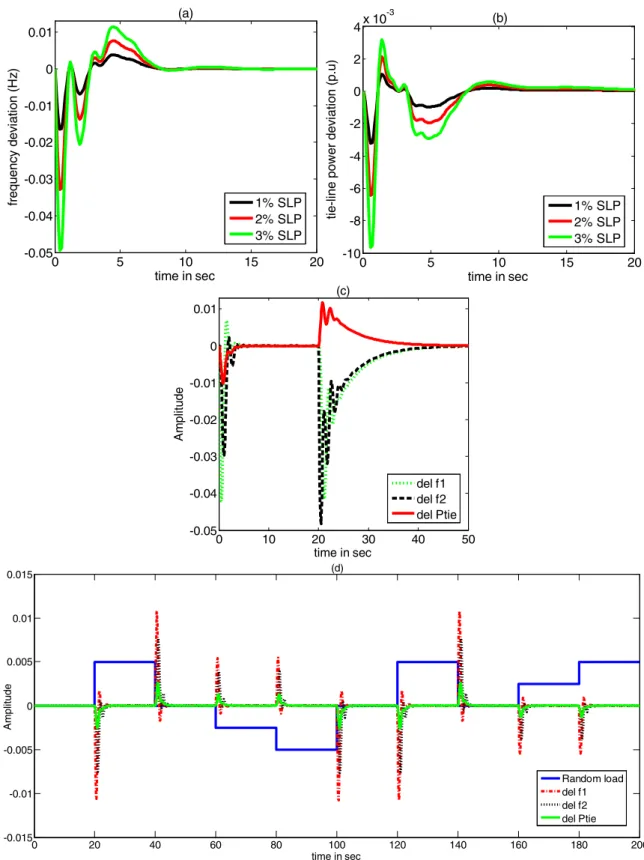
0 5 10 15 20 -0.05 -0.04 -0.03 -0.02 -0.01 0 0.01 time in sec fr equency devi at ion (H z) (a) 1% SLP 2% SLP 3% SLP 0 5 10 15 20 -10 -8 -6 -4 -2 0 2 4x 10 -3 time in sec ti e-l in e pow er devi a ti on (p. u ) (b) 1% SLP 2% SLP 3% SLP 0 10 20 30 40 50 -0.05 -0.04 -0.03 -0.02 -0.01 0 0.01 time in sec A m p lit u d e (c) del f1 del f2 del Ptie 0 20 40 60 80 100 120 140 160 180 200 -0.015 -0.01 -0.005 0 0.005 0.01 0.015 time in sec A m p lit u d e (d) Random load del f1 del f2 del Ptie

Fig. 7.Transient performances of test system-1 under different loading conditions, (a) change in frequency, (b) change in tie-line power, (c) withDPD1¼2%att¼0 s and

Table 5A

Sensitivity analysis of test system-1 with QOGWO algorithm (after returning the controller gains).

Parameters % of change Controller gains ITAE value Settling time (s)

Ki1 Ki2 Kp1 Kp2 Kd1 Kd2 Df1 Df2 DPtie Nominal No change 1.9911 0.0173 1.9325 0.1801 0.1373 0.0998 0.1078 7.62 6.78 17 Loading condition þ50 1.9660 0.0067 1.9962 0.1492 0.2801 0.1740 0.1529 7.74 6.96 17.8 þ25 1.9746 0.0385 1.9515 0.3301 0.1935 0.1755 0.1439 7.44 8.94 18.3 25 1.9390 0.0121 1.9270 0.2502 0.1428 0.1933 0.0795 7.54 8.49 17.6 50 1.7649 0.0836 1.9073 0.0728 0.2375 0.0636 0.0729 8.31 7.11 17.35 Tsg þ50 1.9916 0.0137 1.9900 0.1533 0.2686 0.1650 0.1048 7.67 6.88 16.47 þ25 1.9807 0.0003 1.9593 0.0939 0.2157 0.1713 0.1011 7.79 6.94 15.9 25 1.9891 0.0386 1.9248 0.2913 0.0989 0.1476 0.1127 7.56 8.85 17.2 50 1.9517 0.0371 1.9969 0.3209 0.0261 0.1603 0.1104 7.67 8.89 17.4 Tt þ50 1.9438 0.0121 1.9939 0.2510 0.2358 0.1724 0.1117 7.16 11.53 16.38 þ25 1.9812 0.0112 1.9909 0.1395 0.2682 0.1790 0.1050 7.36 11.38 16.4 25 1.9810 0.0205 1.9741 0.1910 0.0904 0.1704 0.1024 7.78 7.04 17.02 50 1.9961 0.0049 1.9817 0.0303 0.0673 0.1837 0.0972 8.34 7.59 16.58 Tr þ50 1.9135 0.0447 1.9718 0.2561 0.1683 0.1932 0.1257 7.91 11.7 20.3 þ25 1.9917 0.0677 1.9820 0.3616 0.1603 0.1873 0.1205 7.58 9.09 19.3 25 1.9842 0.0206 1.9038 0.1576 0.1863 0.1872 0.1012 7.34 8.52 11.27 50 1.9936 0.0754 1.9867 0.4096 0.1858 0.1716 0.1062 9.42 9.19 11.3 Kr þ50 1.9893 0.0141 1.9916 0.4728 0.2265 0.1626 0.0607 7.44 6.53 10.9 þ25 1.9572 0.0517 1.9232 0.3451 0.0269 0.1347 0.0992 9.3 8.45 13.3 25 1.8522 0.0138 1.9920 0.0648 0.0862 0.1931 0.1617 7.21 8.41 10.79 50 1.9497 0.0141 1.9651 0.0074 0.0431 0.1681 0.1753 8.15 7.04 11.2 Ts þ50 1.9673 0.0311 1.9999 0.0140 0.2776 0.2749 0.1416 10.8 13.9 12.8 þ25 1.9885 0.0118 1.9962 0.1289 0.2133 0.2436 0.1194 9.73 12.9 16.5 25 1.7689 0.0209 1.8560 0.1171 0.2354 0.1070 0.1454 10.11 13.32 17.24 50 1.9911 0.0022 1.9825 0.0023 0.2937 0.2513 0.1317 13.9 14.14 12.68 Kps þ50 1.9576 0.0007 1.9881 0.0344 0.3372 0.3354 0.1169 10.9 11.5 12.8 þ25 1.9441 0.0057 1.8990 0.0072 0.2396 0.2534 0.1223 7.84 7.28 10.05 25 1.9859 0.0049 1.9817 0.0517 0.1827 0.2613 0.1192 7.73 7.09 10.06 50 1.9885 0.0180 1.9707 0.0096 0.3478 0.3846 0.1190 9.27 11.27 12.69 Ri þ50 1.9973 0.0590 1.9809 0.3026 0.2379 0.1784 0.1164 7.07 6.68 11.46 þ25 1.9352 0.0561 1.9682 0.3071 0.1909 0.1423 0.1192 7.68 9.08 16.9 25 1.9949 0.0826 1.9987 0.4167 0.1709 0.1773 0.1211 9.18 9.29 17.74 50 1.9504 0.0119 1.9945 0.0945 0.3210 0.1402 0.1143 7.92 6.85 10.7 Bi þ50 1.9545 0.0053 1.9910 0.1754 0.0254 0.3832 0.1157 8.38 7.93 12.75 þ25 1.9665 0.0139 1.9921 0.0948 0.1304 0.2208 0.1218 7.78 7.24 17.11 25 1.9781 0.0085 1.9510 0.0875 0.1916 0.2614 0.1165 7.71 7.25 17.26 50 1.9879 0.0050 1.9454 0.0731 0.0052 0.3299 0.1167 8.53 7.97 14.45 Table 5B

Sensitivity analysis of test system-1 with QOGWO algorithm (without returning the controller gains).

Parameters % of change ITAE value Settling time Parameters % of change ITAE value Settling time (s)

Df1 Df2 DPtie Df1 Df2 DPtie

Nominal No change Loading condition þ50 0.1217 7.62 6.78 17.02

0.1078 7.62 6.78 17 þ25 0.1147 7.62 6.78 17.02 25 0.0808 7.62 6.78 17.02 50 0.0539 7.62 6.78 17.02 Tt þ50 0.1203 10.2 10.9 15.65 Tsg þ 0.1161 8.62 8.99 11.49 þ25 0.1135 6.99 8 15.19 þ25 0.1107 7.74 6.80 11.5 25 0.1049 7.81 7.07 16.47 25 0.1061 7.67 6.85 16.07 50 0.1043 8.03 7.29 17.22 50 0.1055 7.71 6.93 16.42 Kr þ50 0.0721 8.89 8.09 8.55 Tr þ50 0.1228 7.81 6.89 17.73 þ25 0.0849 8.14 7.26 10.27 þ25 0.1144 7.75 6.85 17.02 25 0.1103 12.94 12.74 17.43 25 0.1022 7.51 8.68 11.31 50 0.1216 12.23 12.05 18.27 50 0.0937 8.57 8.78 10.67 Kps þ50 0.1244 11.01 12.34 17.18 Tps þ50 0.1317 12.89 11.87 18.53 þ25 0.1268 7.57 11.05 19.10 þ25 0.1114 11.87 12.11 16.21 25 0.1106 12.55 13.71 17.02 25 0.1087 10.42 10.67 16.43 50 0.1122 13.9 11.38 18.47 50 0.0967 10.21 10.23 16.36 Bi þ50 0.1014 7.23 10.49 9.04 Ri þ50 0.1221 12.88 11.97 14.70 þ25 0.1002 7.42 6.45 15.02 þ25 0.1177 10.8 11.53 11.37 25 0.1114 10.43 10.02 13.13 25 0.1056 10.67 11.23 13.54 50 0.1220 12.9 12.2 14.02 50 0.1021 10.12 11.05 13.87

algorithms are developed to find optimal values of PID-controller employing ITAE based fitness value. At the end of optimization, controller gains with minimum fitness value (ITAE) and setting time of frequency and tie-line power oscillations are provided in

Table 2. It is evident from Table 2that proposed QOGWO finds minimum fitness value (ITAE = 0.1078) compared to conventional

GWO (ITAE = 0.1216). It is further noted fromTable 2that QOGWO

based PID-controller gives minimum settling time of frequency and tie-line power oscillations compared to GWO algorithm. The comparative transient responses of concerned test system after

load perturbation are depicted inFig. 5and change in ACE with

the said disturbance is given inFig. 6(a). To show the superiority

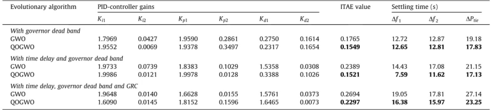
of proposed QOGWO based PID-controller, the numerical simula-tion results obtained with QOGWO tuned PID-controller are Table 6

Optimal value of controller gains, ITAE value and settling time of system oscillations of test system-1 with system nonlinearities.

Evolutionary algorithm PID-controller gains ITAE value Settling time (s)

Ki1 Ki2 Kp1 Kp2 Kd1 Kd2 Df1 Df2 DPtie

With governor dead band

GWO 1.7969 0.0427 1.9590 0.2861 0.2750 0.1614 0.1765 12.72 12.87 19.18

QOGWO 1.9552 0.0069 1.9378 0.3497 0.2317 0.1654 0.1549 12.65 12.81 17.83

With time delay and governor dead band

GWO 1.9733 0.0739 1.8383 0.1029 1.5358 0.0308 0.2389 14.43 17.08 21.15

QOGWO 1.9986 0.0121 1.9978 0.0128 0.3388 0.1026 0.1521 7.59 11.62 17.13

With time delay, governor dead band and GRC

GWO 1.9648 0.0140 1.6628 0.0155 1.5761 0.0373 0.2694 19.05 17.81 27.14

QOGWO 1.6090 0.0145 1.8152 0.1596 1.6465 0.0073 0.2297 16.38 15.97 23.25

Bold signifies best results.

0

5

10

15

-20

-15

-10

-5

0

5

x 10

time in sec

(a)

GWO

QOGWO

0

5

10

15

20

-0.02

-0.015

-0.01

-0.005

0

0.005

0.01

time in sec

(b)

GWO

QOGWO

0

5

10

15

20

-3

-2

-1

0

1

x 10

time in sec

ti

e

-lin

e

p

o

we

r d

e

v

ia

tio

n

(

p

.u

.)

(c)

GWO

QOGWO

Fig. 8.Transient performance of test system-1 after 1% SLP in area-1 with GDB nonlinearity (a) change in frequency of area-1, (b) change in frequency of area-2, and (c) change in tie-line power.

compared with those obtained by other intelligent controllers,

namely fuzzy logic[1], ANN[1]and ANFIS[1]which are recently

reported in the literature and comparative results are presented inTable 3andFig. 5. The improvement of system performances

with proposed technique is illustrated in Table 4. It can be

concluded fromFig. 5andTable 4that the proposed QOGWO

algo-rithm based PID-controller outperforms other intelligent

con-trollers as listed inTable 4which clearly suggests that proposed

QOGWO algorithm is quite impressive for studying LFC problem and rest of the paper is studied with QOGWO algorithm.

6.2. Transient analysis under different loading conditions

To explore the tuning ability of proposed QOGWO algorithm, the test system-1 is further investigated under different loading

conditions. In the first phase of analysis, a 2%and 3%step increase

in demand of the area-1 is individually applied at t¼0 s. The

change in frequency and tie-line power after the aforementioned

load perturbations are displayed inFig. 7(a) and (b), respectively.

The times took to settle down the oscillations by the designed

QOGWO based PID-controller, both for 2%and 3%load

perturba-tions, are 7.62 sðDf1Þ, 6.78 sðDf2Þ, and 17.02 sðDPtieÞ, which also

define the robustness of the proposed technique. It is also inferred

fromFig. 7(a) and (b) that proposed QOGWO tuned PID-controller is able to maintain the system stability and effectively attuned the power system oscillations.

In the second phase of analysis, a 2%step load perturbation at

t¼0 s of the first area and 3%step increase in demand of the

sec-ond area att¼20 s is simultaneously considered to identify the

effectiveness of the proposed algorithm. The dynamic behavior of the concerned power system with the said load perturbation is

shown in Fig. 7(c). It is further noticed from Fig. 7(c) that

QOGWO-tuned PID-controller is effectively handling the load dis-turbances and retrieve the system stability quickly.

A realistic random load pattern as shown inFig. 7(d), marked by

the blue color line, is applied to area-1 of test system-1 to demon-strate the robustness and efficacy of proposed QOGWO algorithm. The PID-controller gains obtained at nominal loading condition are considered in this case to appraise the dynamic stability of the

con-cerned power system. The transient responsesðDf1;Df2;DPtieÞwith

this multiple load perturbation are displayed in Fig. 7(d). The

remarkable role of QOGWO algorithm is that after the first oscilla-tion, peak overshoot of frequency and tie-line power oscillations is vanishing very fast and responses attain the steady value speedily.

Thus, it may be concluded fromFig. 7(d) that the effect of multiple

load perturbation on the system stability can effectively control by

0

5

10

15

20

-20

-15

-10

-5

0

5

x 10

time in sec

(a)

QOGWO

GWO

0

5

10

15

20

-0.02

-0.015

-0.01

-0.005

0

0.005

0.01

time in sec

ti

e-l

ine pow

er devi

a

ti

on (p.

u

)

(c)

QOGWO

GWO

Fig. 9.Transient performances of test system-1 after 1% SLP in area-1 with GDB and TD nonlinearities (a) change in frequency of area-1, (b) change in frequency of area-2, and (c) change in tie-line power.

the QOGWO method which in turns increase the relative stability of the power system.

6.3. Sensitivity analysis of test system-1

Robustness is the ability of the system to perform effectively while its variables are changes within a certain tolerable range. Sensitivity analysis is performed to illustrate the robustness of the designed controller by varying operating loading condition

and system parameters. System parameters such as Tsg, Tt, Tr,

Kr;Tps;Kps;Ri;Bi are varied in the range of 50% instep of 25%.

The study is accomplished in two phases, i.e. initially the PID-controller gains are retuned separately by using QOGWO algorithm

employing ITAE based fitness function and then the system dynamics have been investigated without retuning the controller parameters. The optimal controller gains, minimum fitness value and setting time of frequency and tie-line power oscillations with

the new controller settings are given inTable 5A. It is noteworthy

fromTable 5Athat system performances are hardly changes from its nominal settings. In the second phase of sensitivity analysis, authors have considered the optimal PID-controller gains, shown inTable 2, which are commutated at nominal operating condition to identify the robustness of designed controller. The system performances under this parametric uncertainty condition are

given in Table 5B. It is remarkable from Table 5B that fitness

value and settling time of frequency and tie-line power oscillations

Fig. 10a.Presentation of GRC with steam turbine.

0

5

10

15

20

25

30

-0.03

-0.02

-0.01

0

0.01

0.02

time in sec

(a)

GWO

QOGWO

0

5

10

15

20

25

30

-0.03

-0.02

-0.01

0

0.01

time in sec

fr

equency devi

at

ion

(H

z)

(b)

GWO

QOGWO

Fig. 10b.Transient performances of test system-1 after 1% SLP in area-1 with GDB, TD and GRC nonlinearities (a) change in frequency of area-1, (b) change in frequency of area-2, and (c) change in tie-line power.

for system parameter variations are within the acceptable limit and nearly equal to the results got at the nominal condition. Thus,

it may be concluded fromTables 5A and 5Bthat proposed

con-troller is robust enough to work under different uncertainty conditions.

6.4. Test system-1 with different nonlinearities

To validate the acceptability of proposed QOGWO algorithm to cope with nonlinear interconnected power system, the study is extended to a nonlinear two-area hydrothermal power system considering governor dead-band (GDB), time delay of transmission system, and generation rate constraint (GRC) nonlinearities. LFC analysis is essentially a small signal analysis, thus to get a better insight of power system, linearized model of said nonlinearities are included in the present study. Three different cases are

consid-ered in this phase to appraise the performance of QOGWO algo-rithm. The considered cases are:

Case 1 Transient study including GDB

Case 2 Transient analysis with GDB and time delay

nonlinearities

Case 3 Lastly, considering GDB, time delay, and GRC.

In all the above-mentioned cases, 1%ð0:01p:u:Þstep load change

in area-1 is taken into consideration to identify the stability of the system and to study the consequence effects of aforesaid nonlinearities. The proposed PID controller is optimally designed employing QOGWO algorithm using the same method as described

in Section5.

Governor dead-band (GDB) is defined as the total magnitude of sustained speed change, within which there is no resulting change

0

5

10

15

-15

-10

-5

0

5

x 10

time in sec

fr

equency devi

at

io

n

in

H

z

(a)

GWO

QOGWO

PID [13]

Fuzzy [13]

ann [13]

0

5

10

15

-12

-10

-8

-6

-4

-2

0

2

4

x 10

time in sec

fr

equency

devi

at

io

n i

n

H

z

(b)

GWO

QOGWO

PID [1]

Fuzzy [1]

ANN [1]

0

5

10

15

-12

-10

-8

-6

-4

-2

0

2

4

x 10

time in sec

fr

equency devi

at

io

n

in

H

z

(c)

GWO

QOGWO

PID [1]

Fuzzy [1]

ann [1]

0

5

10

15

-12

-10

-8

-6

-4

-2

0

2

4

x 10

time in sec

fr

equency devi

at

io

n

in

H

z

(d)

GWO

QOGWO

PID [1]

Fuzzy [1]

ANN [1]

Fig. 12.Transient responses of test system-2 after 1% SLP in area-1, (a) frequency deviation in area-1, (b) frequency deviation in area-2, (c) frequency deviation in area-3, (d) frequency deviation in area-4.

Table 7

Optimum values of controller parameters of test system-2.

Controller gains Area-1 Area-2 Area-3 Area-4 ITAE value

Kp1 Ki1 Kd1 Kp2 Ki2 Kd2 Kp3 Ki3 Kd3 Kp4 Ki4 Kd4

GWO 0.5359 0.8189 0.7230 0.6816 0.9869 0.0803 0.1667 0.1551 0.5824 0.4960 0.3623 0.3468 0.0257

QOGWO 0.9916 0.9528 0.6707 0.9581 0.9957 0.2540 0.0043 0.1019 0.1963 0.4381 0.3968 0.1987 0.0245

in the valve position. Typically, backlash type of nonlinearity with

limiting value 0.06% is used to represent the GDB[52]. The effect of

GDB is considered by describing function method and linearized model of same is integrated into the test system-1. The linearized model (transfer function) of speed governor with GDB is

high-lighted by(16) [52]. GsgðsÞ ¼ 0:2 pisþ0:8 1þsTsg ð 16Þ

The optimal solution of PID-controller with QOGWO algorithm

is furnished inTable 6. To show the advantage of QOGWO

algo-rithm, the test system is also examined with conventional GWO

algorithm and optimal controller gains are displayed in Table 6.

Fig. 8defines the dynamic behavior of proposed controller of test

system-1 with GDB. It is noticed from Table 6 that objective

function and settling time values are further minimized with QOGWO algorithm compare to original GWO algorithm that proves the effectiveness of proposed method.

0

5

10

15

20

-10

-8

-6

-4

-2

0

x 10

time in sec

ti

e-l

ine pow

e

r devi

a

ti

on i

n

p.

u.

(e)

GWO

QOGWO

PID [1]

Fuzzy [1]

ANN [1]

0

5

10

15

20

-1

0

1

2

3

4

x 10

time in sec

ti

e-l

ine pow

e

r devi

a

ti

on i

n

p.

u.

(f)

GWO

QOGWO

PID [1]

Fuzzy [1]

ANN [1]

0

5

10

15

20

-0.5

0

0.5

1

1.5

2

2.5

3

3.5

4

x 10

time in sec

ti

e-l

ine pow

e

r devi

at

io

n i

n

p.

u.

(g)

GWO

QOGWO

PID [1]

Fuzzy [1]

ANN [1]

0

5

10

15

-0.5

0

0.5

1

1.5

2

2.5

3

3.5

4

x 10

time in sec

ti

e-l

ine pow

e

r devi

at

io

n i

n

p.

u.

(h)

GWO

QOGWO

PID [1]

Fuzzy [1]

ANN [1]

Fig. 13.Transient responses of test system-2 after 1% SLP in area-1, (a) tie-line power deviation in area-1, (b) tie-line power deviation in area-2, (c) tie-line power deviation in area-3, (d) tie-line power deviation in area-4.

Table 8

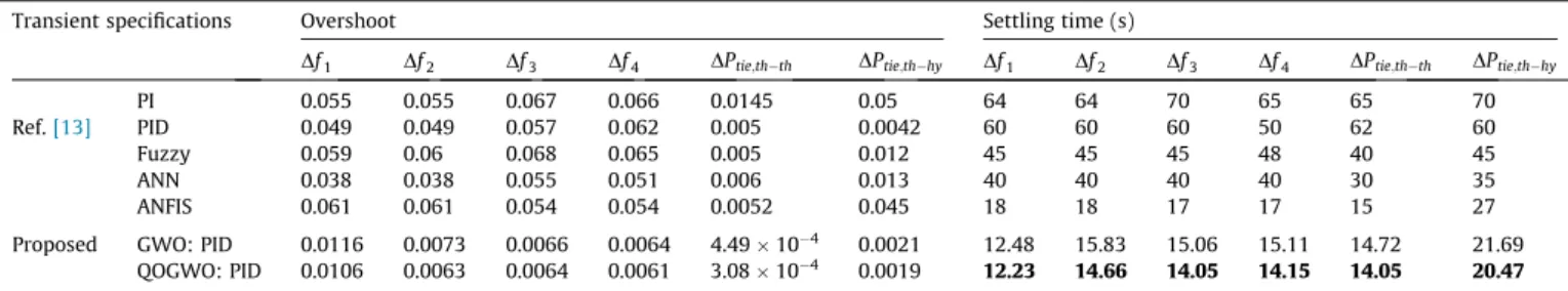
Comparative system performances of test system-2.

Transient specifications Overshoot Settling time (s)

Df1 Df2 Df3 Df4 DPtie;thth DPtie;thhy Df1 Df2 Df3 Df4 DPtie;thth DPtie;thhy

PI 0.055 0.055 0.067 0.066 0.0145 0.05 64 64 70 65 65 70

Ref.[13] PID 0.049 0.049 0.057 0.062 0.005 0.0042 60 60 60 50 62 60

Fuzzy 0.059 0.06 0.068 0.065 0.005 0.012 45 45 45 48 40 45

ANN 0.038 0.038 0.055 0.051 0.006 0.013 40 40 40 40 30 35

ANFIS 0.061 0.061 0.054 0.054 0.0052 0.045 18 18 17 17 15 27

Proposed GWO: PID 0.0116 0.0073 0.0066 0.0064 4.49104 _{0.0021 12.48 15.83 15.06 15.11 14.72 21.69}

QOGWO: PID 0.0106 0.0063 0.0064 0.0061 3.08104

0.0019 12.23 14.66 14.05 14.15 14.05 20.47

The time delay is another most imperative type of nonlinearity encountered in the physical system. The effect of time delay is measured by second order Pade approximation and linear model of same have been included in the system for observation. The

lin-earized form of time delay is available in [49]. For the present

study, the value ofTdis considered as 40 ms. The signals of closed

loop system, i.e. Df₁;Df₂;DPtie, for the concerned power system

with time-delay and GDB nonlinearity are supplied inFig. 9. The

optimal controller gains, minimum ITAE value and settling time

of frequency and tie-line power are available inTable 6. Critical

observation ofFig. 9andTable 6reveals that the responses with

conventional GWO algorithm is suffer from large settling time and unwanted oscillations. Conversely, the signals obtained with QOGWO algorithm based PID-controller takes small time to settle down the oscillations and thus increasing the dynamic stability of power system.

Generation rate constraint (GRC) imposes a practical limit on the generation of power system mainly because of the presence of thermal and mechanical constraints. In usual practice, a limiter is included with steam turbine to represent the GRC as shown in

Fig. 10a. The addition of limiters with the steam turbine is quite realistic because in the electrical system power always generated at a specified rate. For the present study, thermal system is

consid-ered with GRC of 3%/minð0:0005p:u:Þand hydro plant of 270%/min

ð0:045p:u:Þfor upper generation and 360%/minð0:06p:u:Þfor

low-ering generation. The optimal solution of PID-controller using QOGWO algorithm in view of all the said three nonlinearities is

presented inTable 6. The responses of the proposed controller in

terms of frequency deviation inHz and tie-line power deviation

inp:u:are depicted inFig. 10b. To establish the supremacy of

pro-posed QOGWO algorithm, the dynamic responses are compared

with conventional GWO algorithm and provided inFig. 10b. It is

clearly identify fromFig. 10a and bandTable 6that the response

with GWO algorithm requires high settling time to reach the steady value. The improvement of fitness value and settling time with QOGWO algorithm are, in order, 14.74% (ITAE), 14.02%

ðDf1Þ, 10.33%ðDf2Þ, and 14.33%ðDPtieÞ:Thus, it may be concluded

from the aforesaid discussion that the designed controller is cap-able of providing sufficient damping to the system oscillations in the presence of nonlinearities and hence, the robustness of the controller is also verified.

6.5. Test system-2

To investigate the computational efficacy of QOGWO algorithm, the study is extended to a complex and realistic system, namely four-area hydrothermal system. Area-1 and area-2 consist of reheat type thermal power plant whereas area-3 and area-4 Table 9

Percentage of improvement of system performances with QOGWO algorithm for test system-2. Controller

structure System performances

Overshoot Settling time (s) ITAE value

Df1 Df2 Df3 Df4 DPtie;thth DPtie;thhy Df1 Df2 Df3 Df4 DPtie;thth DPtie;thhy

PI 80.73 88.54 90.44 90.75 97.8 96.2 80.8 77.09 79.9 78.2 78.4 70.76 NA Ref.[13] PID 78.4 87.1 88.7 90.8 93.8 54.8 79.6 75.6 76.6 71.7 77.3 65.88 NA Fuzzy 82 89.5 90.6 90.6 93.8 84.17 72.8 67.4 68.8 70.5 64.8 54.51 NA ANN 72.1 83.4 88.4 88 94.8 85.4 71.8 63.4 64.8 64.6 53.17 41.5 NA ANFIS 82.6 89.6 88.1 88.7 94.1 95.8 32.06 18.56 17.35 16.76 6.33 24.19 NA Proposed GWO: PID 8.62 13.69 3.03 4.68 31.4 9.52 2 7.39 6.71 6.35 4.55 5.62 4.67 Table 10

Sensitivity analysis of test system-2 with.

Parameters % of change ITAE value Settling time (s)

Df1 Df2 Df3 Df4 DPtie;thth DPtie;thhy

Nominal No change 0.0245 12.23 14.66 14.05 14.15 14.05 20.47 Tt þ50 0.0258 12.19 15.62 12.88 14.93 16.81 21.73 þ25 0.0248 11.84 14.07 13.66 14.50 17.46 20.03 25 0.0247 12.48 15.03 14.57 14.73 18.69 21.26 50 0.0251 13.03 15.56 14.98 15.24 19.39 21.87 Kr þ50 0.0131 8.20 13.14 12.76 12.82 12.54 15.85 þ25 0.0185 11.10 14.33 14.18 14.32 16.50 19.25 25 0.0228 11.71 13.23 12.88 13.35 18.34 17.19 50 0.0273 9.54 9.33 11.03 10.67 17.95 17.33 Kps þ50 0.0241 11.45 14.11 13.76 13.74 18.37 16.33 þ25 0.0242 11.75 14.35 13.89 13.94 18.20 15.95 25 0.0249 12.41 14.57 14.23 14.11 17.79 15.91 50 0.0259 12.53 14.41 13.85 13.59 17.47 14.83 Tsg þ50 0.0250 12.52 16.19 13.56 15.56 17.59 22.02 þ25 0.0247 11.74 14.84 13.97 14.29 17.81 20.69 25 0.0244 12.23 14.65 14.19 14.34 18.23 20.86 50 0.0245 12.41 14.76 14.29 14.46 18.39 21.01 Tr þ50 0.0247 14.10 17.35 16.84 16.99 13.32 8.10 þ25 0.0297 13.20 16.08 15.55 15.68 19.81 15.09 25 0.0199 10.69 12.51 12.30 12.62 15.92 16.03 50 0.0158 8.94 10.77 10.13 10.24 13.34 15.22 Tps þ50 0.0251 12.45 14.29 14.16 14.49 17.69 20.07 þ25 0.0248 12.35 14.37 14.17 14.47 17.82 20.55 25 0.0242 11.64 14.14 13.94 14.21 18.30 20.89 50 0.0240 11.02 13.91 13.56 13.58 18.61 21.12

consists of hydro-power plant. The transfer function model of test

system is available inFig. 11 [13]and nominal system parameters

are listed inTable 1A. The optimal controller parameters obtained

by the proposed approach is given inTable 7. It is clear fromTable 7

that for the same system with similar controller structure,

mini-mum ITAE value is obtained with QOGWO algorithm

(ITAE = 0.0245) compared to conventional GWO (ITAE = 0.0257). This again proves that QOGWO is better in terms of computational

0

5

10

15

20

-12

-10

-8

-6

-4

-2

0

2

x 10

time in sec

(a)

+50% of Nominal

+25% of Nominal

-25% of Nominal

-50% of Nominal

Nominal

0

5

10

15

20

-12

-10

-8

-6

-4

-2

0

2

4

x 10

time in sec

(b)

+50% of Nominal

+25% of Nominal

-25% of Nominal

-50% of Nominal

Nominal

0

2

4

6

8

10

12

14

-14

-12

-10

-8

-6

-4

-2

0

2

x 10

time in sec

(c)

+50% of Nominal

+25% of Nominal

-25% of Nominal

-50% of Nominal

Nominal

0

2

4

6

8

10

12

14

-14

-12

-10

-8

-6

-4

-2

0

2

x 10

time in sec

(d)

+50% of Nominal

+25% of Nominal

-25% of Nominal

-50% of Nominal

Nominal

0

5

10

15

20

-12

-10

-8

-6

-4

-2

0

2

x 10

time in sec

(e)

+50% of Nominal

+25% of Nominal

-25% of Nominal

-50% of Nominal

Nominal

0

5

10

15

20

-15

-10

-5

0

5

x 10

time in sec

(f)

+50% of Nominal

+25% of Nominal

-25% of Nominal

-50% of Nominal

Nominal

Fig. 14.Sensitivity analysis of test system-2 (deviation of area-1 frequency after load perturbation) (a) variation ofTsg, (b) variation ofTt, (c) variation ofTps, (d) variation of