UC Riverside
UC Riverside Electronic Theses and Dissertations
Title
Semi-Parametric Mixture Models Through Log-Concave Density Estimation
Permalink
https://escholarship.org/uc/item/71k1d4h3Author
Zhou, YangmeiPublication Date
2019 Peer reviewed|Thesis/dissertationUNIVERSITY OF CALIFORNIA RIVERSIDE
Semi-Parametric Mixture Models Through Log-Concave Density Estimation
A Dissertation submitted in partial satisfaction of the requirements for the degree of
Doctor of Philosophy in Applied Statistics by Yangmei Zhou September 2019 Dissertation Committee:
Prof. Weixin Yao, Chairperson Prof. Subir Ghosh
Copyright by Yangmei Zhou
The Dissertation of Yangmei Zhou is approved:
Committee Chairperson
Acknowledgments
I would like to take this opportunity to express my sincere gratitude toward my advisor, Prof. Weixin Yao, for his detailed guidance, encouragement and support through the journey of my Ph.D. research, which is full of obstacles and challenges and yet so exciting and rewarding.
I am so grateful to my dissertation committee member, Prof. Subir Ghosh and Prof. Esra Kurum, for their continuous support and encouragement.
I would also like to thank all the professors and staffs for their guidance and assistance, thank my friends and colleagues I have worked with in the statistics department.
ABSTRACT OF THE DISSERTATION
Semi-Parametric Mixture Models Through Log-Concave Density Estimation by
Yangmei Zhou
Doctor of Philosophy, Graduate Program in Applied Statistics University of California, Riverside, September 2019
Prof. Weixin Yao, Chairperson
This dissertation consists of two parts. The first part considers a semi-parametric two-component mixture model with one component completely known. Assuming the den-sity of the unknown component to be log-concave, which contains a very broad family of densities, we develop a semi-parametric maximum likelihood estimator and propose an EM algorithm to compute it. Our new estimation method finds the mixing proportion and the distribution of the unknown component simultaneously. We establish the identifiability of the proposed semi-parametric mixture model and prove the existence and consistency of the proposed estimators. We further compare our estimator with several existing estima-tors through simulation studies and apply our method to two real data sets from biological sciences and astronomy.
The second part of this dissertation considers the model g(x) = (1−p)f0(x;θ) +
pf(x), where θ represents the unknown parameters of a known distribution f0 , and f represents the distribution of possible outliers. We propose two innovative algorithms to estimateθnonparametrically. The first method is called Minimum Search, which is based on
identifiability of the mixture model. A strong sufficient condition is proposed for the model to be identifiable and a weaker condition is given for the model to be locally identifiable. The second estimator is the maximum likelihood estimator, which is obtained by EM algorithm assuming f is log-concave. Extensive simulation studies show that our methods give very promising performances.
Contents
List of Figures x
List of Tables xi
1 Maximum Likelihood Estimation of a Semiparametric Two-component
Mixture Model using Log-concave Density Estimation 1
1.1 Introduction . . . 1
1.2 Identifiability . . . 4
1.3 Maximum Likelihood Estimation . . . 7
1.3.1 Algorithm . . . 8
1.3.2 Theoretical Properties . . . 9
1.4 Simulation . . . 12
1.5 Real Data Application . . . 19
1.5.1 Prostate Data . . . 19
1.5.2 Carina Data . . . 22
1.6 Discussion . . . 23
1.7 Appendix . . . 25
1.7.1 Theoretical Proof . . . 25
1.7.2 More Simulation Result . . . 35
1.7.3 Source code . . . 42
2 Robust Maximum Likelihood Estimation Based on Semiparametric Mix-ture Models 47 2.1 Introduction . . . 47 2.2 Identifiability . . . 49 2.3 Proposed Algorithms . . . 51 2.3.1 Minimum search . . . 51 2.3.2 EM log-concave method . . . 53 2.4 Theoretical Properties . . . 55
2.4.1 Consistency of (ˆpmin)n and ˆθn. . . 55
2.4.2 Existence and consistency of our maximum likelihood estimator . . . 55
2.6 Discussion . . . 64
2.7 Appendix . . . 65
2.7.1 EM log-concave algorithm . . . 65
2.7.2 Sketch of proofs . . . 70
2.7.3 More simulation results . . . 75
2.7.4 Source code . . . 79
List of Figures
1.1 (a): MSE of the estimates of p when p = 0.2, n = 1000; (b): MSE of the estimates of µwhen p= 0.2, n= 1000. . . 19 1.2 Plots for the prostate data: (a) Histogram of thep-values. The horizontal line
represents the Uniform(0,1) distribution. (b) Plot of the estimated density ˆ
f by our maximum likelihood estimation via EM algorithm. (c) Plot of the estimated density ˆf by the method of [21]. . . 22 1.3 Histogram of RV data overlaid with the estimated two components from our
List of Tables
1.1 Bias (MSE) of estimates ofp/µand mean of the classification error for model 1 when n= 1000. . . 15 1.2 Bias (MSE) of estimates ofp/µand mean of the classification error for model
2 when n= 1000. . . 15 1.3 Bias (MSE) of estimates ofp/µand mean of the classification error for model
3 when n= 1000. . . 16 1.4 Bias (MSE) of estimates ofp/µand mean of the classification error for model
4 when n= 1000. . . 16 1.5 Bias (MSE) of estimates ofp/µand mean of the classification error for model
5 when n= 1000. . . 17 1.6 Bias (MSE) of estimates ofp/µand mean of the classification error for model
6 when n= 1000. . . 17 1.7 Bias (MSE) of estimates ofp/µand mean of the classification error for model
7 when n= 1000. . . 18 1.8 Estimates of pfor the prostate cancer data. . . 21 1.9 Estimates of pfor the Carina data. . . 23 1.10 Bias(MSE) of estimates ofp/µand mean of the classification error for model
1 when n= 250. . . 35 1.11 Bias(MSE) of estimates ofp/µand mean of the classification error for model
1 when n= 500. . . 35 1.12 Bias(MSE) of estimates ofp/µand mean of the classification aerror for model
2 when n= 250. . . 36 1.13 Bias(MSE) of estimates ofp/µand mean of the classification error for model
2 when n= 500. . . 36 1.14 Bias(MSE) of estimates ofp/µand mean of the classification error for model
3 when n= 250. . . 37 1.15 Bias(MSE) of estimates ofp/µand mean of the classification error for model
3 when n= 500. . . 37 1.16 Bias(MSE) of estimates ofp/µand mean of the classification error for model
4 when n= 250. . . 38 1.17 Bias(MSE) of estimates ofp/µand mean of the classification error for model
1.18 Bias(MSE) of estimates ofp/µand mean of the classification error for model 5 when n= 250. . . 39 1.19 Bias(MSE) of estimates ofp/µand mean of the classification error for model
5 when n= 500. . . 39 1.20 Bias(MSE) of estimates ofp/µand mean of the classification error for model
6 when n= 250. . . 40 1.21 Bias(MSE) of estimates ofp/µand mean of the classification error for model
6 when n= 500. . . 40 1.22 Bias(MSE) of estimates ofp/µand mean of the classification error for model
7 when n= 250. . . 41 1.23 Bias(MSE) of estimates ofp/µand mean of the classification error for model
7 when n= 500. . . 41 2.1 Bias (MSE) of estimates of p/θ and mean of dL2 and dKL for the model 1
when n= 500. . . 61 2.2 Bias (MSE) of estimates of p/θ/µ1 and mean of dL2 and dKL for the model
2 when n= 500. . . 61 2.3 Bias (MSE) of estimates of p/θ/µ1 and mean of dL2 and dKL for the model
3 when n= 500. . . 62 2.4 Bias (MSE) of estimates of p/θ/µ1 and mean of dL2 and dKL for the model
4 when n= 500. . . 62 2.5 Bias (MSE) of estimates of p/θ/µ1 and mean of dL2 and dKL for the model
5 when n= 500. . . 63 2.6 Bias (MSE) of estimates of p/θ and mean of dL2 and dKL for the model 6
when n= 500. . . 63 2.7 Bias (MSE) of estimates of p/θ and mean of dL2 and dKL for the model 7
when n= 500. . . 64 2.8 Bias(MSE) of estimates ofp/θand mean ofdL2anddKLwhenp= 0,n= 250,
K = 200. . . 75 2.9 Bias(MSE) of estimates of p/θ/µ1 and mean of dL2 and dKL when p= 0.2,
n= 250,K = 200. . . 76 2.10 Bias(MSE) of estimates ofp/θ/µ1 and mean of dL2 and dKL when p= 0.2,
n= 250,K = 200. . . 76 2.11 Bias(MSE) of estimates ofp/θ/µ1 and mean of dL2 and dKL when p= 0.2,
n= 250,K = 200. . . 77 2.12 Bias(MSE) of estimates ofp/θ/µ1 and mean of dL2 and dKL when p= 0.2,
n= 250,K = 200. . . 77 2.13 Bias(MSE) of estimates of p/θ and mean of dL2 and dKL when p0 = 0.8,
p1 = 0.05,p2= 0.15, n= 250, K= 200. . . 78 2.14 Bias(MSE) of estimates of p/θ and mean of dL2 and dKL when p0 = 0.8,
Chapter 1
Maximum Likelihood Estimation of
a Semiparametric Two-component
Mixture Model using Log-concave
Density Estimation
1.1
Introduction
In this chapter, we consider the following two-component mixture model,
where the probability density function (pdf)f0(x) is known, whereas the mixing proportion
p ∈ [0,1] and the pdf f are unknown. Model (2.1) is motivated by studies in biological sciences to cluster differentially expressed genes in microarray data, see [2]. Typically for microarray data, we build a test statistic, say Ti, for each gene i. Under the null hypothesis, which presumes no difference in expression levels under two or more conditions, Ti is assumed to have a known distribution (in general Student’s t or Fisher). Under the alternative hypothesis, the distribution is unknown. Thus, the distribution of the test statistic can be described by model (2.1) where p is the proportion of non-null statistics. The estimation of pand the pdff can tell us the probabilityPi that geneiis differentially expressed givenTi=ti:
Pi = pf(ti)
(1−p)f0(ti) +pf(ti) .
[2] considered model (2.1) assumingf to be symmetric. They obtained some identifiability results under moment and symmetry conditions.
[30] considered another special case,
g(x) = (1−p)φσ(x) +pf(x)
where f0 =φσ is a normal density with mean 0 and unknown standard deviation σ. This model was inspired by sequential clustering [29], which finds candidates for centers of clusters first, then carries out a local search to find the objects that belong to those clusters, and finally selects the best cluster. The algorithm repeats after the best cluster is being removed. [30] proposed an EM-type estimator and a maximizing π-type estimator for their model
which can be easily extended to models wheref0 is not normal. A slightly different model is considered by [35]:
g(x) = (1−p)f0(x;ξ) +pf(x−µ),
where ξ is a possibly unknown parameter, and µ is a non-null location parameter for f. They proposed a new effective estimator based on the minimum profile Hellinger distance (MPHD). They established the existence and uniqueness of their estimator and also proved its consistency under some regularity conditions. Their method does not require f to be symmetric and thus can be applied to more general models. For some other alternative estimators, see, for example [21, 16].
In this chapter, we propose to estimate (2.1) using a new approach by imposing a fairly general log-concave shape constraint on f, i.e. log(f) ∈ Φ; here Φ denotes the family of concave functions φ on R which are upper semicontinuous and coercive in the sense that φ(x) → −∞, as |x| → ∞. Note that log(f) needs to be coercive in order for f to be a density function. The family of log-concave densities [7, 8] is very broad and contain many commonly used parametric families of distributions, such as normal distribution, exponential distribution, logistic distribution, etc. We propose to estimate the new model by maximizing a semiparametric mixture likelihood. Compared to the kernel density estimation of f used by many existing methods [2, 35, 16], the new method does not require the choice of one or more bandwidths [26]. We establish the identifiability of the proposed semiparametric mixture model and prove the existence and consistency of the proposed estimators. We further compare our estimator with several existing estimators
through simulation studies and apply our method to two real data sets from biological sciences and astronomy.
The rest of the chapter is organized as follows. In Section 2.2 we discuss some iden-tifiability issues for model (2.1). Section 1.3 introduces our maximum likelihood estimator and a detailed EM type algorithm. Existence and consistency properties of our estimator are established. Section 2.5 demonstrates the finite sample performance of our proposed estimator by comparing with many other existing algorithms. Two real data applications are given in Section 1.5. Section 2.6 gives a brief discussion. The Appendix in Section 2.7 contains the detailed proofs.
1.2
Identifiability
Note that the model (2.1) is non-identifiable without any constraint on the density f, see e.g., [2], and [21]. However, a parametric model for f might create biased or even misleading statistical inference when the model assumption is incorrect. In this chapter, we impose a general log-concave shape constraint on f(x), i.e. f(x) = eφ(x), where φ(x) is a concave function. Log-concave densities attracted lots of attention in the recent years since it is very flexible and can be estimated by nonparametric maximum likelihood estimator without requiring the choice of any tuning parameter. For more details, see [5], [8], [34], [9] and the review of the recent progress in log-concave density estimation by [26].
We first provide a lemma which can be easily proved by extending the result of Lemma 4 of [21].
Lemma 1.2.1. The model (2.1) is identifiable if there exists asuch that lim x→a+ f(x) f0(x) = 0 or lim x→a− f(x) f0(x) = 0.
Remark 1.2.1. Proposition 1.2.1 also holds if a = ±∞, and this result is more general (requiring weaker condition) than the result of Proposition 3(i) of [2].
Remark 1.2.2. Proposition 1.2.1 guarantees that model (2.1) is identifiable if the support of f is strictly contained in the support of f0 and the two supports have different Legesgue
measure.
If log(f) is assumed to be log-concave, we can have the following result with the proof provided in Section 2.7.
Proposition 1.2.1. Assume f0 >0 and log(f)∈Φ. Model (2.1) is identifiable if either of
the following two conditions are satisfied
1. φ(x)−logf0(x)→ −∞ asx→+∞ or x→ −∞.
2. |logf0(x)|=O(|x|k), for some 0< k <1.
Next we provide some examples to demonstrate how to use the above results to establish the identifiability of the model (2.1).
Example 1.2.1. If f0(x) is the density of a t distribution with ν degrees of freedom, and
f is log-concave, then model (2.1) is identifiable. Proof. Since f0(x) = Γ(ν+12 ) √ νπΓ(ν2)(1 + x2 ν ) −ν+12 , we have, log(f0(x)) = log(Γ( ν+ 1 2 ))− 1 2log(νπ)−log(Γ( ν 2))− ν+ 1 2 log(1 + x2 ν ).
Thus, for any 0 < k <1, log(f0(x))/xk→ 0, as x →+∞. Based on Proposition 1.2.1, we can conclude that model (2.1) is identifiable when log(f)∈Φ.
Remark 1.2.3. Similarly, one can check that when f0 is the pdf of an F distribution,
log-normal distribution, or Pareto distribution, then model (2.1) is identifiable under the condition that log(f)∈Φ.
Remark 1.2.4. Example 1.2.1 ensures Model 7 from Section 2.5 is identifiable.
Example 1.2.2. Suppose f0(x) is the density of a normal distribution with mean µ and
variance σ2, then model (2.1) is identifiable if limx→+∞φx(x2) < −2σ12, or limx→−∞ φx(x2) < − 1
2σ2, or the condition of Remark 1.2.2 holds.
Proof. Suppose limx→+∞φx(x2) <−2σ12, or limx→−∞φx(x2) <−2σ12. Since
φ(x)−logf0(x) = φ(x) + log( √ 2πσ) + 1 2σ2(x−µ) 2 = x2(φ(x) x2 + 1 x2log( √ 2πσ) + 1 2σ2(1− µ x) 2) → −∞, asx→+∞ orx→ −∞. Hence f(x) f0(x)
→0 as x→+∞orx→ −∞, and Proposition 1.2.1 asserts the identifiability of model (2.1).
Remark 1.2.5. Under the constraints set by Example 1.2.2, Model 1, 4, and 5 from Section 2.5 are identifiable.
Example 1.2.3. Suppose f0(x) is the density of an exponential distritution with rate λ,
holds.
Proof. Suppose limx→+∞φ(xx) <−λ. Since,
φ(x)−logf0(x) = φ(x)−logλ+λx = x(φ(x) x − logλ x +λ) → −∞, asx→+∞. Hence f(x) f0(x)
→ 0 as x → +∞, and again Proposition 1.2.1 ensures the identifiability of model (2.1).
Remark 1.2.6. Under the constraints set by Example 1.2.3, Model 3 from Section 2.5 is identifiable.
1.3
Maximum Likelihood Estimation
Suppose we have a random sample of n i.i.d. observations X1, X2,· · · , Xn from the densityg(x) = (1−p)f0(x) +pf(x),p∈[0,1], andf =eφ is a log-concave density, i.e.,
φ∈Φ. For any distributionQon R, we define,
L(p, φ;Q) =
Z
log((1−p)f0+peφ)dQ.
Then, with the empirical distribution Qn = 1 n
n
X
i=1
δXi , where δXi is the degenerate
semiparametric log likelihood, L(p, φ;Qn) = 1 n n X i=1 log((1−p)f0(Xi) +peφ(Xi)), (1.2)
subject to the condition thatR
eφ(x)dx= 1. The log-likelihood (1.2) is semiparametric since it contains both the parameter pand the nonparametric component φ.
1.3.1 Algorithm
Maximizing the semiparametric log likelihood (1.2) is not trivial. To this end, we propose an EM algorithm [6] to maximizeL(p, φ;Qn).
Algorithm 1.3.1. Staring from initial values p(0) and f(0), iterating the following E step and M step until convergence.
E step Given p(k) and f(k), find the classification probabilities
ωi(k+1)= (1−p (k))f 0(xi) (1−p(k))f 0(xi) +p(k)f(k)(xi) , i= 1, . . . , n.
M step Given ωi(k+1), update the parameterp and the nonparametric concave function φ,
p(k+1)= 1 n n X i=1 (1−ωi(k+1)), φ(k+1) = arg max φ∈Φ,R eφ(x)dx=1 n X i=1 (1−ω(ik+1))φ(xi), f(k+1)=eφ(k+1).
In the M step, we find φ(k+1) using an active set algorithm, which is described in [7] and implemened in the R package logcondens by [25]. Throughout this chapter, we use “EM logconcave” to represent the above algorithm. The following result establishes the monotone properties of our EM logconcave algorithm.
Proposition 1.3.1. Let `(k) =Pn i=1 log((1−p(k))f 0(xi) +p(k)eφ (k)(x i)), where p(k) and φ(k) are kth update in Algorithm 1.3.1, then
`(k+1)≥`(k),
for anyk≥0.
1.3.2 Theoretical Properties
For the existence of a maximizer of L(p, φ;Q) for a general distribution Q, we follow the approach of [9]. We define the convex support ofQ as,
csupp(Q) =\{C:C⊆ R closed and convex, Q(C) = 1}.
Theorem 1.3.1. For fixedf0, assumesupp{f0} ⊆csupp(Q), and there exists some integer
k≥1, such that,
Z
|x|kQ(dx)<∞ and interior(csupp(Q))6=∅.
For some fixed m(x) = c0ec1|x|
k
, c0, c1 > 0. Let Φ =˜ {φ ∈ Φ :
R
eφ(x)dx = 1 and f 0(x) ≤
m(x)eφ(x)}. Then
L(Q) = sup
p∈[0,1], φ∈Φ˜
L(p, φ, Q)
is real and there exists
(p0, φ0)∈ argmax
p∈[0,1],φ∈Φ˜
L(p, φ;Q).
Moreover,
interior(csupp(Q))⊆dom(φ0) ={x∈ R:φ0(x)>−∞} ⊆csupp(Q).
The proof of Theorem 2.4.3 is given in the Appendix (Section 2.7).
Example 1.3.1. Assume f0 represents the standard normal density. Consider all the
log-concave normal densities with mean µ and standard deviation σ. Suppose µ and σ are bounded. Then, for integer k = 2, there exist c0, c1 > 0, such that Φ˜ contains all such
normal pdfs with meanµand standard deviationσ. In addition, Theorem 2.4.3 implies that the maximum of L(p, φ;Q) exists over p∈[0,1]and φ∈Φ˜.
In general, the maximizer of L(p, φ;Q) is not unique. However, if Q has den-sity g0(x) = (1 −p0)f0(x) +p0eφ0(x), where g0(x) is identifiable, then L(p0, φ0;Q) =
R
log(g0(x))g0(x)dx, and this (p0, φ0) is the unique maximizer. This is because as not-ed by [9], if we have (p1, φ1), such that L(Q) = L(p0, φ0;Q) = L(p1, φ1;Q), let g1(x) = (1−p1)f0(x) +p1eφ1(x), then,
Z
Note the above integral is exactly the Kullback-Leibler divergence which is positive and equals 0 iffg0 =g1 almost everywhere. Thus (p0, φ0) = (p1, φ1) except thatφ0 and φ1 may differ on a set of Lebesgue measure zero.
Next we establish the consistency of our maximum likelihood estimator. First, we introduce some notations,
Qk = {Q onR:
Z
|x|kQ(dx)<∞},
Q0 = {Q onR: interior(csupp(Q))6=∅}.
In the remainder of this section, we consider the convergence of distributions under Mallows’ distance D1 [17]. Specifically, for two distributionsQ,Q0 ∈ Qk,
Dk(Q, Q0) = inf X, X0
X∼Q, X0∼Q0
{E|X−X0|k}1/k.
It is known that lim
n→∞ Dk(Qn, Q) → 0 is equivalent to Qn →w Q and
R
|x|kQn(dx) →
R
|x|kQ(dx) [1, 17]. HereQ
n→w Qmeans weak convergence, or convergence in distribution. Now we are ready to state our main consistency theorem.
Theorem 1.3.2. Assume, (a). supp{f0} ⊆csupp(Q); (b). for some fixed integer k≥ 1,
the unknown density f satisfies the following condition: ∃ m(x) =c0ec1|x|
k
, where ci > 0,
i= 0,1, such that,f0(x)≤m(x)f(x) =m(x)eφ(x). Let {Qn} be a sequence of distributions
in Q0TQk such that lim
n→∞ Dk(Qn, Q) = 0 for some Q ∈ Q0
TQk. Suppose f
semi-continuous and log(f0)
1 +|x| is bounded. Then
lim
n→∞L(Qn) =L(Q).
Assume there exist maximizers (pn, φn) of L(p, φ;Qn), and a unique maximizer(p∗, φ∗) of L(p, φ;Q), where pn, p∗∈[0,1], φn, φ∗ ∈Φ˜. Let fn= exp(φn), f∗ = exp(φ∗), then
lim n→∞pn = p ∗ , lim n→∞, x→y fn(x) = f ∗ (y), ∀y∈ R \∂{f∗>0}, limsup n→∞, x→y fn(x) ≤ f∗(y), ∀y∈∂{f∗ >0}, lim n→∞ Z |fn(x)−f∗(x)|dx = 0,
here ∂{f∗ >0} represents the boundary of the set {f∗ >0}.
Practically, Qn will be the empirical distribution function which automatically satisfies the above assumption. Based on the above theorem, we can know that the proposed semiparametric maximum likelihood estimators of pand f are consistent.
Remark 1.3.1. Theorem 2.4.3 and Theorem 2.4.4 still holds if we consider the distribution
Q to be defined on Rd, with d= 1,2,3,· · · .
1.4
Simulation
In this section, we investigate the finite sample performance of our algorithm and compare it to the estimator proposed by [21] ( ˆα0.1kn
estimator by [2], the EM-type estimator and Maximizing-π type estimator by [30], and the Minimum profile Hellinger distance estimator by [35].
In order to test our method under different settings, we simulateK = 200 samples of n i.i.d. random variables with the common distribution given by the following seven models:
• Model 1: g(x) = (1−p)N(µ= 0, σ= 2) +pN(µ= 3, σ= 1),
• Model 2: g(x) = (1−p)·unif(0,1) +p·beta(α= 1, β= 5),
• Model 3: g(x) = (1−p)·exp(λ= 1) +p·(exp(λ= 1) + 2),
• Model 4: g(x) = (1−p)N(0,1) +p(χ2(3) + 2),
• Model 5: g(x) = (1−p)N(0,1) +p·(exp(λ= 0.5) + 3),
• Model 6: g(x) = (1−p)N(0,1) +p·(t(d.f.= 5) + 3),
• Model 7: g(x) = (1−p)·tdf=5+p·logistic(location = 5,scale = 0.5).
For each sample we estimate p, the meanµof the unknown component f and the classification error. For our algorithm and the algorithm by [35], final estimators ˆp and ˆf are always produced, thus the estimated probability ˆwi that the i-th observation is from the known component f0(x), given Xi =xi, can be calculated by
ˆ wi =
(1−pˆ)f0(xi) (1−pˆ)f0(xi) + ˆpfˆ(xi)
.
by the following, ˆ wi = 2(1−pˆ)f0(xi) (1−pˆ)f0(xi) + ˆh(xi) ,
where ˆh is the kernel density estimator of g with Gaussian kernel and Silverman’s “rule of thumb” bandwidth [28]. Note that the algorithm proposed by [21] actually can estimatef when f is non-increasing. But we find that the algorithm works best when f0 and f have the same support and it often produces unreliable estimates when the two supports differ from each other. Thus, we do not use ˆf to estimate ˆwi for [21]’s algorithm even when the true f does decrease on its support, instead, we follow [30]’s recommendation to get ˆwi.
The algorithms by [35] and [2] give a final mean estimator ˆµ directly. For other methods, after we get ˆwi, we estimate µby the following weighted sum,
ˆ µ= Pn i=1(1−wiˆ)Xi Pn i=1(1−wˆi) .
Last, we report the classification error (CE) based on ˆwi as the mean squared error between ˆ
wi and the true wi, i.e.,
CE = 1 n n X i=1 ( ˆwi−wi)2,
where wi = 1 if xi is from the known component f0(x) and 0 if xi is from the unknown component f(x).
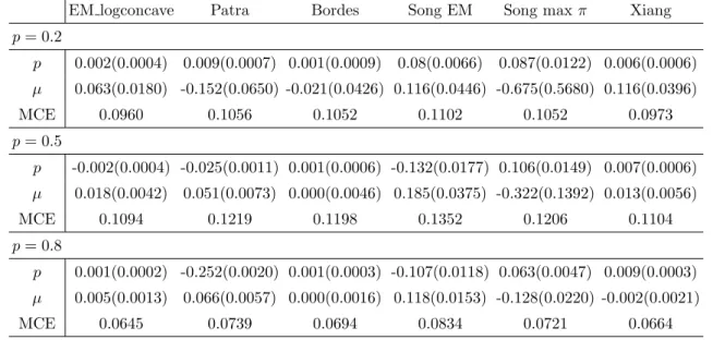
For model 1, Table 1 reports the bias and MSE of the estimates of p, the bias and MSE of the estimates ofµ, and the mean of the classification error (MCE) for different methods over K = 200 repetitions when p = 0.2, p = 0.5, and p = 0.8, with sample size n = 1000. Similar reports of other models can be found in Tables 2.2 — 2.7. Simulation
results for sample sizes n= 250 and n= 500 are reported in the Appendix (Section 2.7). We report the results of [2]’s algorithm only for model 1, 2, 6 and 7, because this method fails when f(x) is not symmetric.
Table 1.1: Bias (MSE) of estimates of p/µand mean of the classification error for model 1 when n= 1000.
EM logconcave Patra Bordes Song EM Song max π Xiang
p= 0.2 p 0.002(0.0004) 0.009(0.0007) 0.001(0.0009) 0.08(0.0066) 0.087(0.0122) 0.006(0.0006) µ 0.063(0.0180) -0.152(0.0650) -0.021(0.0426) 0.116(0.0446) -0.675(0.5680) 0.116(0.0396) MCE 0.0960 0.1056 0.1052 0.1102 0.1052 0.0973 p= 0.5 p -0.002(0.0004) -0.025(0.0011) 0.001(0.0006) -0.132(0.0177) 0.106(0.0149) 0.007(0.0006) µ 0.018(0.0042) 0.051(0.0073) 0.000(0.0046) 0.185(0.0375) -0.322(0.1392) 0.013(0.0056) MCE 0.1094 0.1219 0.1198 0.1352 0.1206 0.1104 p= 0.8 p 0.001(0.0002) -0.252(0.0020) 0.001(0.0003) -0.107(0.0118) 0.063(0.0047) 0.009(0.0003) µ 0.005(0.0013) 0.066(0.0057) 0.000(0.0016) 0.118(0.0153) -0.128(0.0220) -0.002(0.0021) MCE 0.0645 0.0739 0.0694 0.0834 0.0721 0.0664
Table 1.2: Bias (MSE) of estimates of p/µand mean of the classification error for model 2 when n= 1000.
EM logconcave Patra Bordes Song EM Song maxπ Xiang
p= 0.2 p -0.008(0.0014) -0.023(0.0015) -0.015(0.0012) -0.15(0.0228) 0.382(0.1496) 0.017(0.0019) µ -0.018(0.0015) 0.027(0.0016) -0.029(0.0017) -0.014(0.0007) 0.199(0.0401) -0.007(0.0010) MCE 0.1270 0.1520 0.1511 0.1676 0.1847 0.1339 p= 0.5 p 0.001(0.0007) -0.046(0.0030) -0.040(0.0024) -0.248(0.0811) 0.228(0.0548) -0.047(0.0035) µ -0.003(0.0001) -0.011(0.0002) -0.032(0.0011) -0.038(0.0015) 0.077(0.0064) -0.022(0.0012) MCE 0.1609 0.1990 0.1974 0.2638 0.1887 0.1753 p= 0.8 p -0.001(0.0004) -0.074(0.0059) -0.070(0.0055) -0.311(0.0974) 0.099(0.0105) -0.060(0.0043) µ -0.001(0.00004) -0.019(0.0004) -0.033(0.0011) -0.040(0.0016) 0.025(0.0007) -0.030(0.0014) MCE 0.1000 0.1264 0.1261 0.2103 0.1129 0.1142
Table 1.3: Bias (MSE) of estimates of p/µand mean of the classification error for model 3 when n= 1000.
EM logconcave Patra Bordes Song EM Song max π Xiang p= 0.2 p 0.001(0.0002) -0.001(0.0006) NA -0.060(0.0038) 0.410(0.1698) 0.024(0.0011) µ 0.006(0.0082) -0.039(0.0152) NA 0.048(0.0149) -1.140(1.3094) -0.105(0.0184) MCE 0.0709 0.0851 NA 0.0879 0.1568 0.0790 p= 0.5 p 0.000(0.0003) -0.013(0.0006) NA -0.073(0.0057) 0.259(0.0681) 0.042(0.0028) µ 0.003(0.0021) -0.011(0.0030) NA 0.018(0.0030) -0.502(0.2578) -0.091(0.0157) MCE 0.0595 0.0767 NA 0.0790 0.1166 0.0732 p= 0.8 p 0.001(0.0002) -0.228(0.0010) NA -0.231(0.0012) 0.104(0.0112) 0.071(0.0060) µ -0.001(0.0013) -0.002(0.0014) NA -0.002(0.0014) -0.159(0.0283) -0.104(0.0224) MCE 0.0260 0.0325 NA 0.0322 0.0526 0.0617
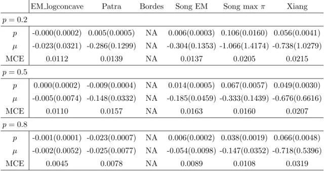
Table 1.4: Bias (MSE) of estimates of p/µand mean of the classification error for model 4 when n= 1000.
EM logconcave Patra Bordes Song EM Song max π Xiang p= 0.2 p -0.000(0.0002) 0.005(0.0005) NA 0.006(0.0003) 0.106(0.0160) 0.056(0.0041) µ -0.023(0.0321) -0.286(0.1299) NA -0.304(0.1353) -1.066(1.4174) -0.738(1.0279) MCE 0.0112 0.0139 NA 0.0137 0.0205 0.0215 p= 0.5 p 0.000(0.0002) -0.009(0.0004) NA 0.014(0.0005) 0.067(0.0057) 0.049(0.0030) µ -0.005(0.0074) -0.148(0.0332) NA -0.185(0.0459) -0.333(0.1439) -0.676(0.6616) MCE 0.0110 0.0157 NA 0.0163 0.0160 0.0207 p= 0.8 p -0.001(0.0001) -0.023(0.0007) NA 0.006(0.0002) 0.038(0.0019) 0.066(0.0048) µ -0.002(0.0052) -0.025(0.0077) NA -0.054(0.0098) -0.147(0.0352) -0.718(0.5396) MCE 0.0045 0.0078 NA 0.0089 0.0108 0.0319
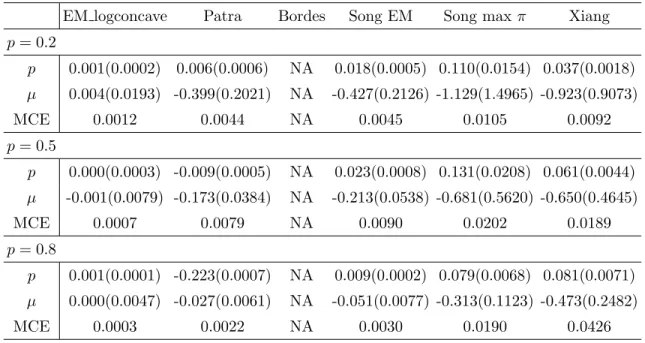
Table 1.5: Bias (MSE) of estimates of p/µand mean of the classification error for model 5 when n= 1000.
EM logconcave Patra Bordes Song EM Song max π Xiang p= 0.2 p 0.001(0.0002) 0.006(0.0006) NA 0.018(0.0005) 0.110(0.0154) 0.037(0.0018) µ 0.004(0.0193) -0.399(0.2021) NA -0.427(0.2126) -1.129(1.4965) -0.923(0.9073) MCE 0.0012 0.0044 NA 0.0045 0.0105 0.0092 p= 0.5 p 0.000(0.0003) -0.009(0.0005) NA 0.023(0.0008) 0.131(0.0208) 0.061(0.0044) µ -0.001(0.0079) -0.173(0.0384) NA -0.213(0.0538) -0.681(0.5620) -0.650(0.4645) MCE 0.0007 0.0079 NA 0.0090 0.0202 0.0189 p= 0.8 p 0.001(0.0001) -0.223(0.0007) NA 0.009(0.0002) 0.079(0.0068) 0.081(0.0071) µ 0.000(0.0047) -0.027(0.0061) NA -0.051(0.0077) -0.313(0.1123) -0.473(0.2482) MCE 0.0003 0.0022 NA 0.0030 0.0190 0.0426
Table 1.6: Bias (MSE) of estimates of p/µand mean of the classification error for model 6 when n= 1000.
EM logconcave Patra Bordes Song EM Song max π Xiang
p= 0.2 p -0.010(0.0003) -0.007(0.0006) 0.083(0.0012) -0.022(0.0006) 0.077(0.0080) 0.001(0.0003) µ 0.171(0.0455) 0.029(0.0262) -0.075(0.0843) 0.083(0.0257) -0.414(0.2369) 0.001(0.0177) MCE 0.0440 0.0450 0.0455 0.0457 0.0468 0.0435 p= 0.5 p 0.001(0.0003) -0.031(0.0015) -0.002(0.0006) -0.053(0.0031) 0.038(0.0028) -0.002(0.0631) µ -0.010(0.0115) 0.148(0.0264) -0.003(0.0066) 0.182(0.0375) -0.020(0.0185) 0.018(0.0066) MCE 0.0094 0.0672 0.0658 0.0680 0.0656 0.0631 p= 0.8 p -0.001(0.0001) -0.059(0.0037) -0.002(0.0004) -0.063(0.0043) 0.008(0.0006) 0.001(0.0034) µ -0.004(0.0072) 0.169(0.0307) -0.001(0.0024) 0.174(0.0321) 0.055(0.0073) -0.003(0.0034) MCE 0.0046 0.0637 0.0570 0.0643 0.0567 0.0545
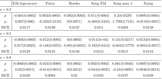
Table 1.7: Bias (MSE) of estimates of p/µand mean of the classification error for model 7 when n= 1000.
EM logconcave Patra Bordes Song EM Song maxπ Xiang
p= 0.2 p -0.001(0.0002) 0.003(0.0004) -0.002(0.0003) 0.011(0.0004) 0.2(0.0529) 0.0095(0.0004) µ 0.007(0.006) -0.423(0.2122) 0(0.0071) -0.468(0.2455) -1.799(3.7131) -0.0116(0.0057) MCE 0.0117 0.0139 0.0137 0.014 0.0403 0.0138 p= 0.5 p -0.003(0.0003) -0.012(0.0005) 0(0.0003) 0.014(5e-04) 0.131(0.0217) 0.0134(0.0004) µ 0.017(0.0023) -0.148(0.0255) -0.001(0.0022) -0.192(0.0413) -0.683(0.5779) -0.0041(0.0017) MCE 0.0129 0.0145 0.0146 0.0151 0.0315 0.0144 p= 0.8 p -0.0060(0.0002) -0.024(0.0008) 0(0.0002) 0.002(0.0002) 0.061(0.0046) 0.0097(0.0002) µ 0.02(0.0015) -0.014(0.0015) 0(0.0012) -0.044(0.0035) -0.24(0.0695) 0.0046(0.0013) MCE 0.0103 0.0094 0.01 0.0101 0.0197 0.0108
The simulation results demonstrate that our method has the overall best perfor-mance among all methods. In addition, our method is even more favorable when the sample size n gets larger. Overall, all the estimates of µ get better when p gets larger, which is expected because we are getting more points from the unknown component. [2]’s method does not work well whenf is not symmetric due to the fact that their algorithm is based on the symmetry of f. [35]’s method has excellent performance whenf is symmetric, because their algorithm incorporates the symmetry property of f in these cases. When f is not symmetric, our algorithm is far superior. [21]’s method works better whenp is small, but it only estimatesf when it is decreasing.
To better display our simulation results, we also plot the MSE of point estimates of p and µ vs. different models for all the methods we mentioned above when p = 0.2 and n = 1000, except for the method by [2] as their method fails to estimate p and µ for
half of the models we discussed here. Figure 1.1 shows that the curve representing our method always lies at the bottom for all seven models considered, which demonstrates the effectiveness of our new method.
0.00 0.05 0.10 0.15 2 4 6 model MSE method EM_logconcave Patra Song_EM song_maxpi Xiang (a) MSE of the p estimator
0 1 2 3 2 4 6 model MSE method EM_logconcave Patra Song_EM song_maxpi Xiang (b) MSE of the mean estimator
Figure 1.1: (a): MSE of the estimates of p when p = 0.2, n = 1000; (b): MSE of the estimates of µwhen p= 0.2, n= 1000.
1.5
Real Data Application
1.5.1 Prostate Data
In this section we consider the prostate data consisting of genetic expression levels related to prostate cancer patients of [10]. The data set is a 6033×102 matrix, with entries xij = expression level for gene i on patient j, i = 1,· · ·, n, j = 1,· · · , m, here, n = 6033, m = 102. Among the m = 102 patients, m1 = 50 of them are normal control
subjects (corresponding toj = 1,· · · , m1) andm2 = 52 of them are prostate cancer patients (corresponding toj =m1+ 1,· · ·, m2). The goal of the study is to discover the potential genes that are differentially expressed between normal control and prostate cancer patients.
Two-sample t-test is performed to test the significance of each geneiby,
ti = (¯xi(1)−xi¯(2))/si, where ¯xi(1) = ( m1 P j=1 xij)/m1, ¯xi(2) = ( m2 P j=m1+1 xij)/m2,s2i = (1/m1+1/m2) ( m1 P j=1 (xij−x¯i(1))2+ m2 P j=m1+1 (xij −xi¯ (2))2 )
/(m−2). These two-sided t-tests produce n= 6033 p-values, and the distribution of thesep-values under the null hypothesis (i.e., the gene is not differentially expressed) has a uniform density, while under the alternative hypothesis (i.e., the gene is differentially expressed) has a non-increasing density.
The estimation of p is reported in Table 1.8. We can see that the estimate by [2] and the Maximizing-π type estimate by [30] give a relatively big estimate. The estimate procedure by [2] assumes the density function under the alternative hypothesis to be sym-metric, while in our example this density is non-increasing, which violates the symmetric assumption. (If we apply [2]’s method to the original t statistics directly, the estimate of p is ˆp= 0.0072.) It is known that the Maximizing-π type estimator by [30] tends to over-estimate thep value, which can also be seen in Table 1.8. We also want to point out that several approaches have been proposed by [10] to estimatepas well, the estimator based on central matching method gives ˆp= 0.020 (please see [10] and [11] for detailed description of those estimators), and Table 1.8 shows that our estimator gives a closest value to Efron’s result.
Table 1.8: Estimates ofp for the prostate cancer data. EM logconcave Patra Bordes Song EM Song max π Xiang
0.0173 0.0817 0.1975 0.0076 0.6132 0.1915
Figure 1.2 plots the estimated density ˆf based on our method and the method by [21]. It can be seen that our estimate of the density ˆf tends to have a much smaller support compared to the one given by [21]. Note that small p-values indicate the support for the alternative hypothesis. Therefore, it makes sense that the support of f for this prostate data may be much smaller than (0,1).
Frequency 0.0 0.2 0.4 0.6 0.8 1.0 0 50 100 150 200 250 (a) pvalues 0.000 0.004 0.008 0.012 0 100 200 300 400 500 density EM_logconcave (b) 0.0 0.2 0.4 0.6 0.8 1.0 0 5 10 15 20 density Patra (c)
Figure 1.2: Plots for the prostate data: (a) Histogram of the p-values. The horizontal line represents the Uniform(0,1) distribution. (b) Plot of the estimated density ˆf by our maximum likelihood estimation via EM algorithm. (c) Plot of the estimated density ˆf by the method of [21].
1.5.2 Carina Data
Carina is one of the seven dwarf spheroidal (dSph) satellite galaxies of Milkey Way. Here we consider the data consisting of radial velocities (RV) ofn= 1266 stars from Carina galaxy. The data is obtained by Magellan and MMT telescopes ([33]). The stars of Milkey
Way contribute contamination to this data set. We assume the distributionf0 of RV from stars of Milkey Way is known and follows the Besancon Milky Way model ([23]). We would like to analyze this data set to better understand the inhomogeneous distribution of the RV of stars in Carina galaxy.
The estimation of pis reported in Table 1.9. We see that the estimation by [30]’s Maximizing-π type estimator gives a relatively big estimate. Other estimates are relatively close.
Table 1.9: Estimates of pfor the Carina data. EM logconcave Patra Bordes Song EM Song max π Xiang
0.354 0.364 0.363 0.370 0.687 0.385
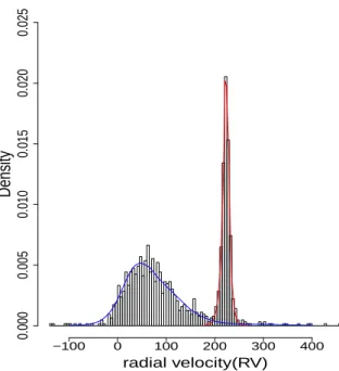
In Figure 1.3, we plot the histogram of the RV data overlaid with our estimated two components of the mixture density. Based on the plot, we can see that our estimation approximates the data fairly well. The component corresponding to the stars of Carina looks very symmetric, and in fact astronomers usually assume the distribution to be Gaussian, which makes the density estimation proposed by [21] fail.
1.6
Discussion
In this chapter we study the two-component mixture model with one component completely known. A semiparametric maximum likelihood estimator is developed via EM
Density −100 0 100 200 300 400 0.000 0.005 0.010 0.015 0.020 0.025 radial velocity(RV)
Figure 1.3: Histogram of RV data overlaid with the estimated two components from our EM log-concave algorithm
algorithm and log-concave approximation. Unlike most existing estimation procedures, our new method finds the mixing proportion and the distribution of the unknown component simultaneously without any selection of a tuning parameter and the proposed EM algorithm satisfies the non-decreasing property of the traditional EM algorithm. We establish the existence of consistency of the proposed estimator. Simulation results show that our method is more favorable than many other competing estimation methods.
In this chapter, we assume that the first component is completely known, it would be our interest to apply our method to a more general model where the componentf0 also contains some unknown parameter and extend our method to the regression setting.
1.7
Appendix
1.7.1 Theoretical Proof
Proof of Lemma 1.2.1. According to [21], if we let G, F0, and F be the cumulative distribution functions of g, f0 and f respectively, define p0 = inf{γ ∈ (0,1] : [G−(1−
γ)F0]/γ is a CDF}, then
p0 =p{1−essinf
f f0
},
where essinf(h) = sup{t∈ R :m{x :h(x) < t} = 0}, and here m represents the Lebesgue measure. Now if essinfff
0 > 0, there must exist some t >0, such that, m{x :
f(x)
f0(x) < t}=
0, i.e., ff(x)
0(x) ≥ t almost everywhere, which contradicts to the fact that limx→a+
f(x)
f0(x) =
0 or limx→a− f(x)
f0(x) = 0. Hence we can conclude that essinf
f
f0 = 0, and consequently
p0 =p, which means if we can write g(x) = (1−p)f0(x) +pf(x), this pis fixed and equals
p0. Consequently f(x) = (g(x)−(1−p)f0(x))/p is fixed as well, and our model (2.1) is identifiable.
Proof of Proposition 1.2.1. Since f(x) =eφ(x) is a log-concave density, there exist con-stants aand b >0, such thatφ(x)≤a−b|x|(see [4]), which implies
φ(x)−logf0(x)≤a−b|x| −logf0(x).
Now if|logf0(x)|=O(|x|k), for some 0< k <1, apparently,
Hence φ(x)−logf0(x) → −∞ as x → +∞ or x → −∞, which shows limx→+∞ff(x) 0(x) = 0.
Thus, model (2.1) is identifiable from Proposition 1.2.1.
Proof of Theorem 2.4.3. SupposeR|x|kQ(dx)<∞, interior(csupp(Q))6=∅,R
eφ(x)dx= 1 and f0(x) ≤ m(x)eφ(x). For any concave function φ satisfying the above condition-s, there exist (a0, b0), such that φ(x) ≤ a0 −b0|x|, thus for any p 6= 0, L(p,−b0|x| − log(R e−b0|x|dx);Q)≥log p
R
e−b0|x|dx−b0
R
|x|Q(dx)>−∞, thus we haveL(Q)>−∞. When maximizingL(p, φ;Q) over allφ∈Φ, we may restrict our attention to functions˜ φsuch that dom(φ) ={x ∈ R :φ(x) >−∞} ⊆csupp(Q). For if dom(φ) *csupp(Q), replacing φ(x)
with−∞for allx /∈csupp(Q), then the value ofL(p, φ−log(R eφ(x)dx);Q) would be greater or equal to the original L(p, φ;Q). Note that since supp(f0) = csupp(Q), the new concave function φ0 = φ−log(Reφ(x)dx) still satisfies the conditions above, i.e., Reφ0(x)dx = 1, f0(x)≤m(x)eφ
0(x)
and dom(φ0) ={x∈ R:φ(x)>−∞} ⊆csupp(Q). We denote Φ(Q) to be the family of all φ∈Φ with dom(˜ φ) ={x∈ R:φ(x)>−∞} ⊆csupp(Q).
Now we show that L(Q) < ∞. Suppose that φ ∈ Φ(Q) is such that M = maxx∈Rdφ(x) > 0. Let Dt = {φ ≥ t}, hence Dt is closed and convex. For any α > 0,
we have the following estimate,
L(p, φ;Q) = Z log((1−p)f0+peφ)dQ ≤ Z log((1−p)m(x) +p)Q(dx) + Z φdQ ≤ Z log(m(x) + 1)Q(dx)−αM Q(Rd\D−αM) +M Q(D−αM) = Z log(m(x) + 1)Q(dx)−(α+ 1)M( α α+ 1−Q(D−αM)).
Note that R
log(m(x) + 1)Q(dx) exists since R
|x|kQ(dx) <∞. By Lemma 4.1 of [9], for any fixed α,
Leb(D−αM) ≤ (1 +α)dMde−M/
Z (1+α)M
0
tde−tdt
= (1 +α)dMde−M/(d! +o(1))→0, asM → ∞.
Lemma 2.1 of [9] says that for sufficiently large α and sufficiently small δ > 0, there exist some sufficiently small >0, such that,
sup{Q(C) :C ⊆ Rclosed and convex, Leb(C)≤δ}< α α+ 1−,
which implies that L(p, φ;Q) → −∞, as M → ∞. Since for any φ ∈ Φ(Q), we also have L(p, φ;Q) ≤ R
log((1−p)m(x) +p)dQ+M, ⇒ L(Q) < ∞ and there exist constants M0 and M∗, such that
L(Q) = sup p∈[0,1], φ∈Φ(Q)
M0≤max(φ(x))≤M∗
L(p, φ;Q).
Now that we knowL(Q) is real, we are ready to prove the existence of a maximizer (p0, φ0) of L(Q). Let (pn, φn) be a sequence such that pn ∈ [0,1], φn ∈ Φ(Q), Mn = max(φn(x))∈[M0, M∗], and −∞ < L(pn, φn;Q) ↑L(Q) asn→ ∞. Here we assume {pn} is a convergent sequence, say pn →p0 ∈[0,1], asn → ∞. If {pn} is not convergent, since it is bounded, it must have a convergent subsequence {pnk}, and the sequence {pnk, φnk}
would satisfy all those properties above and we can just simply replace the original sequence with this subsequence.
Next, we show that,
inf
n≥1φn(x0)>−∞, ∀x0 ∈interior(csupp(Q)). (1.3)
For any x0 ∈interior(csupp(Q)), if φn(x0) < Mn, then x0 can not be an interior point of{φn≥φn(x0)}, hence, L(pn, φn;Q) = Z log((1−pn)f0+pneφn)dQ ≤ Z log(m(x) + 1)Q(dx) + Z φndQ ≤ Z log(m(x) + 1)Q(dx) +φn(x0) + (Mn−φn(x0))Q(φn≥φn(x0)) ≤ Z log(m(x) + 1)Q(dx) +φn(x0)(1−h(Q, x0)) + max(Mn,0),
where h(Q, x) = sup{Q(C) :C ⊆Rd closed and convex, x /∈interior(C)} <1 by Lemma 2.13 of [9]. And the above inequalities still hold even ifφn(x0) =Mn. Thus we have,
φn(x0) ≥ L(pn, φn;Q)− R log(m(x) + 1)Q(dx)−max(Mn,0) 1−h(Q, x0) ⇒inf n≥1φn(x0) ≥ L(p1, φ1;Q)− R log(m(x) + 1)Q(dx)−max(M∗,0) 1−h(Q, x0) >−∞,
which establishes (1.3). Sinceφn≤M∗, together with (1.3), Lemma 3.3 of [27] implies that
there exist constantsaand b >0 such that,
Let C = {x ∈ R :liminf
n→∞ φn(x) > −∞} ⊇ interior(csupp(Q)) and ¯φ(x) = a−b|x|, using
Lemma 4.2 of [9], together with (1.3) and (2.8) we can conclude that there exist φ0 ∈ Φd and a subsequence φnk such that C⊆dom(φ0)⊆csupp(Q) and,
limsup k→∞
φnk(x) ≤ φ0(x)≤a−b|x|, ∀x∈ R,
lim
k→∞φnk(x) = φ0(x)>−∞, ∀x∈interior(csupp(Q)).
Since dom(φnk)⊆csupp(Q), we haveφnk converges toφ0almost everywhere as the Lebesgue measure of the boundary of csupp(Q) is zero, then we can concludeR
eφ0(x)dx= 1
by dominated convergence. Thus, φ0 ∈ Φ(Q). Next, we apply Fatou’s Lemma to the nonnegative functions x 7→ R log(m(x) + 1)Q(dx) +a−b|x| −log((1−pnk)f0+pnke φnk), and we get, limsup k→∞ L(pnk, φnk;Q)≤L(p0, φ0;Q). Hence, L(Q)≥L(p0, φ0;Q)≥limsup k→∞ L(pnk, φnk;Q) =L(Q),
which shows (p0, φ0) is the maximizer that we are looking for.
Proof of Theorem 2.4.4. Since lim
n→∞Dk(Qn, Q)→0, hence Qn→w Qand Z |x|kQn(dx)→ Z |x|kQ(dx), asn→ ∞. Suppose limsup n→∞ L(Qn) = λ
such that L(Qnk) →λ. If we let h(x) =−b0|x| −log( R
e−b0|x|dx) as we did in the proof of
Theorem 2.4.3, then, h∈Φ, and for any˜ p >0,
λ ≥ limsup k→∞ L(p, h;Qnk) =limsup k→∞ Z log((1−p)f0+peh)dQnk ≥ logp−b0 Z |x|Q(dx)−log( Z e−b0|x|dx)>−∞.
Note that in the above inequalities, we used the fact that lim n→∞
R
|x|Qn(dx) =
R
|x|Q(dx) by Lemma 4.6 of [27].
Let Mn = maxx∈Rdφn(x). Since lim
n→∞
R
log(m(x) + 1)Qn(dx) =
R
log(m(x) + 1)Q(dx) by Lemma 4.6 of [27], similar to the proof of Theorem 2.4.3, one can show that forn sufficiently large, we haveL(pn, φn;Qn)→ −∞, ifMn→ ∞asn→ ∞, andL(pn, φn;Qn)≤
R
log(m(x) + 1)Q(dx) +Mn, provided that
limsup
n→∞ Qn(Cn)<1, for any
{Cn:Cn⊆ R closed and convex, lim
n→∞Leb(Cn) = 0}. (1.5)
Hence there exist some suitable constants M0 and M∗, such that M0 < Mnk < M∗ for k
sufficiently large and thus λ <∞.
Here we explain how (1.5) is derived. As in the proof of Lemma 2.1 of Schuhmacher, [27], there exist a simplex ˜∆ = conv(˜x0,· · ·,x˜d) with positive Lebesgue measure and open sets U0, U1, · · ·, Ud with Q(Uj) ≥ η > 0, for 0 ≤ j ≤ d, here η = min
0≤j≤d Q(Uj) > 0. For any convex and closed set C with C ∩Uj 6= ∅ for all j, we have ˜∆ ⊆ C. By Theorem 4.4.4 of [3], liminf
n→∞ Qn(Uj) ≥ Q(Uj) ≥ η for all j. Thus if limn→∞ Leb(Cn) = 0, then for
Cn∩Uj =∅,⇒Qn(Cn)≤1−Qn(Uj)≤1− min 1≤j≤dQn(Uj). Since, Qn(Uj) = liminf n→∞ Qn(Uj) +Qn(Uj)−liminfn→∞ Qn(Uj) ≥ η+ inf k≥nQk(Uj)−liminfn→∞ Qn(Uj) =η+o(1), thus min
1≤j≤dQn(Uj)≥η+o(1), which shows thatQn(Cn)≤1−η+o(1), and hence (1.5) is established.
Now that we knowMnk is bounded forksufficiently large, andL(pnk, φnk;Qnk)→
λ∈ R as k→ ∞, we may assume {pnk}, is a convergent sequence, say pnk → p∗ ∈ [0,1],
as k→ ∞. For if {pnk} is not convergent, since it is bounded, it must have a convergent
subsequence {pnkl}, and the sequence {pnkl, φnkl} would satisfy all those properties above and we can just simply replace the original sequence with this subsequence.
Again, as in the proof of Theorem 2.4.3, for anyx0 ∈interior(csupp(Q)), we have,
φnk(x0) ≥ L(pnk, φnk;Qnk)− R log(m(x) + 1)Q(dx)−max(Mnk,0) 1−h(Qnk, x0) .
As Lemma 2.13 of [27] states that limsup n→∞
h(Qnk, x)≤h(Q, x) for any x∈ R, we have,
liminf k→∞ (φnk(x0)) ≥ λ−R log(m(x) + 1)Q(dx)−max(M∗,0) 1−h(Q, x0) >−∞.
Hence, for k large enough,
inf
Again, we can deduce from (1.6) and the boundedness of Mnk that there exist constantsa
and b >0 such that,
φnk(x)≤a−b|x|, ∀ksufficiently large, x∈R
d. (1.7)
Similar as before we conclude that there exist φ∗ ∈Φd and a subsequence{φnkl}such that interior(csupp(Q))⊆dom(φ∗)⊆csupp(Q) and,
limsup l→∞,x→y
φnkl(x) ≤ φ∗(y)≤a−b|y|, ∀y∈ R,
lim
l→∞,x→yφnkl(x) = φ∗(y)>−∞, ∀y∈interior(csupp(Q)).
Then Reφ∗(x)dx= 1 by dominated convergence, which implies that φ∗ ∈Φ.˜
By Skorohod’s theorem, there exist a probability space (Ω,F, P) and random variables Xnkl ∼ Qnkl, X ∼ Q, such that lim
l→∞ Xn = X almost surely. Let Hnkl =
R
Fatou’s Lemma, we have, λ = lim l→∞L(pnkl, φnkl;Qnkl) = liml→∞ Z log((1−pnkl)f0+pnkle φnk l)dQn kl = lim l→∞{ Z log(m(x) + 1)Q(dx) + Z (a−b||x||)Qnkl(dx)−E(Hnkl)} = Z log(m(x) + 1)Q(dx) +a−b Z ||x||Q(dx)−liminf l→∞ E(Hnkl) ≤ Z log(m(x) + 1)Q(dx) +a−b Z ||x||Q(dx)−E(liminf l→∞ (Hnkl)) ≤ E{limsup l→∞ log((1−pnkl)f0(Xnkl) +pnklexp(φnkl(Xnkl)))} ≤ E(log((1−p∗)f0(X) +p∗exp(φ∗(X)))) ≤ L(Q).
In order to show that λ ≥L(Q), we use the approximations φ∗ ≤φ∗() ≤ φ∗(1), 0< ≤1 from Lemma 4.4 of [9], sinceφ∗()∈Φ is Lipschitz continuous, one can show that
|φ∗()|
1+||x|| is bounded, and hence by Lemma 4.6 of [9], we have,
λ = lim k→∞L(pnk, φnk;Qnk) ≥ lim k→∞L(p ∗ , φ∗()−log( Z eφ∗()(x)dx), Qnk) = L(p∗, φ∗()−log( Z eφ∗()(x)dx), Q) = Z log{(1−p∗)f0 Z eφ∗()(x)dx+p∗eφ∗()}dQ−log( Z eφ∗()(x)dx) → Z log((1−p∗)f0+p∗eφ ∗ )dQ=L(p∗, φ∗;Q), as→0.
conver-gence on (1−p∗)f0
R
eφ∗(1)(x)dx+p∗eφ∗(1)−(1−p∗)f0
R
eφ∗()(x)dx−p∗eφ∗(). Thus we have shown thatλ=L(Q), and (p∗, φ∗) = (p∗, φ∗) is the unique maximizer.
With exactly the same argument, we can show that liminf
n→∞ L(Qn) =L(Q) as well,
and henceL(Qn)→L(Q), as n→ ∞.
Also, if we let f∗ = exp◦φ∗,fn= exp◦φn, we have shown that,
lim l→∞pnkl = p ∗, limsup l→∞,x→y fnkl(x) ≤ f∗(y), ∀y ∈∂{f∗>0}, lim l→∞,x→yfnkl(x) = f ∗ (y), ∀y ∈Rd\∂{f∗ >0}.
In particular,{fnkl}converges tof∗ almost everywhere w.r.t. Lebesgue measure and hence
R
|fnkl(x) −f∗(x)|dx → 0, as l → ∞ by dominated convergence. Our proof actually shows that for any subsequence of{Qn}, we can further find a subsequence with the above convergence properties. That means the original sequence must satisfy those properties as well, otherwise we would arrive at contradictions and that completes the proof.
1.7.2 More Simulation Result
Table 1.10: Bias(MSE) of estimates ofp/µ and mean of the classification error for model 1 when n= 250.
EM logconcave Patra Bordes Song EM Song max π Xiang
p= 0.2 p 0.008(0.0019) -0.001(0.0021) 0.018(0.0046) -0.071(0.0057) 0.106(0.0160) 0.021(0.0056) µ 0.057(0.0738) -0.396(0.3286) -0.166(0.2109) -0.108(0.2243) -0.846(0.9437) 0.243(0.1864) MCE 0.1029 0.1094 0.1097 0.1138 0.1104 0.1058 p= 0.5 p 0.000(0.0023) -0.041(0.0036) 0.005(0.0025) -0.130(0.0185) 0.100(0.0153) 0.014(0.0026) µ 0.017(0.0225) 0.023(0.0167) -0.021(0.0198) 0.143(0.0393) -0.344(0.1635) 0.032(0.0208) MCE 0.1151 0.1259 0.1232 0.1379 0.1248 0.1138 p= 0.8 p -0.001(0.0011) -0.070(0.0057) -0.001(0.0014) -0.104(0.0123) 0.056(0.0040) 0.016(0.0014) µ 0.003(0.0072) 0.059(0.0102) -0.001(0.0085) 0.097(0.0158) -0.147(0.0323) -0.008(0.0079) MCE 0.0670 0.0781 0.0722 0.0835 0.0752 0.0703
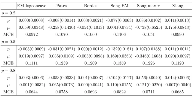
Table 1.11: Bias(MSE) of estimates ofp/µ and mean of the classification error for model 1 when n= 500.
EM logconcave Patra Bordes Song EM Song max π Xiang
p= 0.2 p 0.000(0.0008) -0.008(0.0014) 0.003(0.0021) -0.077(0.0063) 0.086(0.0102) 0.011(0.0013) µ 0.059(0.0348) -0.258(0.1430) -0.054(0.1013) 0.001(0.0734) -0.738(0.6525) 0.175(0.0843) MCE 0.0972 0.1070 0.1060 0.1106 0.1051 0.0990 p= 0.5 p -0.003(0.0009) -0.031(0.0021) 0.000(0.0012) -0.132(0.0181) 0.107(0.0158) 0.011(0.0011) µ 0.019(0.0097) 0.035(0.0109) -0.003(0.0098) 0.169(0.0363) -0.346(0.1605) 0.020(0.0097) MCE 0.1111 0.1239 0.1209 0.1359 0.1226 0.1120 p= 0.8 p 0.003(0.0006) -0.053(0.0033) 0.001(0.0007) -0.104(0.0117) 0.056(0.0040) 0.014(0.0006) µ -0.001(0.0032) 0.065(0.0073) 0.000(0.0041) 0.110(0.0155) -0.121(0.0220) -0.007(0.0040) MCE 0.0644 0.0758 0.0693 0.0822 0.0711 0.0685
Table 1.12: Bias(MSE) of estimates of p/µand mean of the classification aerror for model 2 whenn= 250.
EM logconcave Patra Bordes Song EM Song maxπ Xiang
p= 0.2 p 0.004(0.0051) -0.021(0.0033) -0.006(0.0036) -0.156(0.0248) 0.371(0.1443) 0.056(0.0087) µ -0.022(0.0038) 0.061(0.0073) -0.019(0.0029) 0.013(0.0032) 0.197(0.0401) -0.011(0.0026) MCE 0.1368 0.1554 0.1568 0.1746 0.1858 0.1437 p= 0.5 p 0.004(0.0043) -0.064(0.0071) -0.037(0.0041) -0.300(0.0916) 0.230(0.0576) -0.013(0.0041) µ -0.005(0.0007) -0.004(0.0004) -0.032(0.0013) -0.034(0.0013) 0.080(0.0070) -0.014(0.0011) MCE 0.1678 0.2110 0.2031 0.2778 0.1964 0.1764 p= 0.8 p 0.009(0.0019) -0.105(0.0124) -0.065(0.0057) -0.312(0.1001) 0.081(0.0078) -0.049(0.0056) µ 0.000(0.0002) -0.020(0.0005) -0.033(0.0012) -0.039(0.0016) 0.010(0.0006) -0.018(0.0010) MCE 0.1030 0.1384 0.1266 0.2137 0.1124 0.1140
Table 1.13: Bias(MSE) of estimates ofp/µ and mean of the classification error for model 2 when n= 500.
EM logconcave Patra Bordes Song EM Song maxπ Xiang
p= 0.2 p -0.001(0.0028) -0.021(0.0020) -0.007(0.0022) -0.154(0.0238) 0.379(0.1496) 0.035(0.0047) µ -0.019(0.0024) 0.041(0.0030) -0.025(0.0022) -0.006(0.0008) 0.197(0.0393) -0.009(0.0018) MCE 0.1294 0.1544 0.1520 0.1697 0.1862 0.1369 p= 0.5 p 0.002(0.0022) -0.053(0.0045) -0.039(0.0032) -0.292(0.0860) 0.234(0.0583) -0.034(0.0035) µ -0.004(0.0003) -0.008(0.0002) -0.033(0.0013) -0.037(0.0014) 0.080(0.0069) -0.014(0.0009) MCE 0.1638 0.2031 0.2011 0.2723 0.1940 0.1753 p= 0.8 p 0.003(0.0010) -0.086(0.0081) -0.070(0.0058) -0.312(0.0990) 0.097(0.0102) -0.048(0.0038) µ -0.001(0.0001) -0.020(0.0005) -0.034(0.0012) -0.040(0.0016) 0.024(0.0007) -0.022(0.0010) MCE 0.1001 0.1307 0.1263 0.2119 0.1129 0.1139
Table 1.14: Bias(MSE) of estimates ofp/µ and mean of the classification error for model 3 when n= 250.
EM logconcave Patra Bordes Song EM Song max π Xiang p= 0.2 p 0.005(0.0011) 0.009(0.0021) NA -0.050(0.0034) 0.431(0.1889) 0.048(0.0042) µ 0.026(0.0400) -0.041(0.0581) NA 0.048(0.0591) -1.115(1.2677) -0.139(0.0493) MCE 0.0737 0.0869 NA 0.0895 0.1718 0.0842 p= 0.5 p 0.002(0.0013) -0.019(0.0019) NA -0.069(0.0065) 0.269(0.0742) 0.081(0.0103) µ -0.001(0.0096) -0.001(0.0126) NA 0.013(0.0120) -0.495(0.2618) -0.174(0.0590) MCE 0.0623 0.0806 NA 0.0839 0.1271 0.0860 p= 0.8 p 0.003(0.0007) -0.046(0.0029) NA -0.225(0.0017) 0.107(0.0122) 0.087(0.0096) µ 0.001(0.0052) 0.003(0.0061) NA -0.004(0.0057) -0.157(0.0316) -0.150(0.0446) MCE 0.0274 0.0351 NA 0.0354 0.0589 0.0734
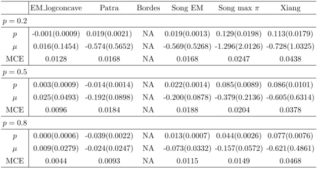
Table 1.15: Bias(MSE) of estimates ofp/µ and mean of the classification error for model 3 when n= 500.
EM logconcave Patra Bordes Song EM Song max π Xiang p= 0.2 p 0.004(0.0005) 0.004(0.0011) NA -0.055(0.0034) 0.415(0.1746) 0.038(0.0024) µ 0.014(0.0204) -0.039(0.0316) NA 0.047(0.0315) -1.119(1.2657) -0.131(0.0357) MCE 0.0722 0.0862 NA 0.0855 0.1610 0.0819 p= 0.5 p 0.001(0.0005) -0.016(0.0010) NA -0.070(0.0057) 0.260(0.0692) 0.060(0.0059) µ 0.004(0.0047) -0.007(0.0061) NA 0.017(0.0064) -0.489(0.2475) -0.126(0.0338) MCE 0.0604 0.0787 NA 0.0811 0.1189 0.0790 p= 0.8 p 0.002(0.0003) -0.036(0.0017) NA -0.029(0.0013) 0.106(0.0115) 0.080(0.0078) µ 0.001(0.0027) 0.001(0.0026) NA -0.002(0.0030) -0.159(0.0294) -0.117(0.0284) MCE 0.0270 0.0334 NA 0.0341 0.0557 0.0677
Table 1.16: Bias(MSE) of estimates ofp/µ and mean of the classification error for model 4 when n= 250.
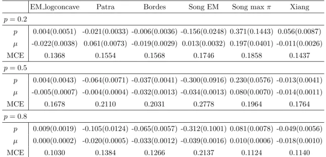
EM logconcave Patra Bordes Song EM Song max π Xiang p= 0.2 p -0.001(0.0009) 0.019(0.0021) NA 0.019(0.0013) 0.129(0.0198) 0.113(0.0179) µ 0.016(0.1454) -0.574(0.5652) NA -0.569(0.5268) -1.296(2.0126) -0.728(1.0325) MCE 0.0128 0.0168 NA 0.0168 0.0247 0.0438 p= 0.5 p 0.003(0.0009) -0.014(0.0014) NA 0.022(0.0014) 0.085(0.0089) 0.086(0.0101) µ 0.025(0.0493) -0.192(0.0898) NA -0.200(0.0878) -0.379(0.2136) -0.605(0.6314) MCE 0.0096 0.0184 NA 0.0188 0.0204 0.0378 p= 0.8 p 0.000(0.0006) -0.039(0.0022) NA 0.013(0.0007) 0.044(0.0026) 0.077(0.0076) µ 0.009(0.0279) -0.024(0.0247) NA -0.073(0.0332) -0.157(0.0572) -0.621(0.4861) MCE 0.0044 0.0093 NA 0.0115 0.0149 0.0468
Table 1.17: Bias(MSE) of estimates ofp/µ and mean of the classification error for model 4 when n= 500.
EM logconcave Patra Bordes Song EM Song max π Xiang p= 0.2 p -0.002(0.0003) 0.009(0.0009) NA 0.010(0.0005) 0.108(0.0141) 0.074(0.0073) µ -0.008(0.0721) -0.410(0.2935) NA -0.404(0.2668) -1.109(1.4363) -0.803(1.1190) MCE 0.0116 0.0151 NA 0.0147 0.0201 0.0271 p= 0.5 p 0.000(0.0005) -0.011(0.0008) NA 0.017(0.0009) 0.074(0.0066) 0.069(0.0062) µ -0.011(0.0244) -0.169(0.0525) NA -0.220(0.0720) -0.374(0.1801) -0.607(0.6089) MCE 0.0095 0.0167 NA 0.0178 0.0178 0.0288 p= 0.8 p 0.002(0.0004) -0.031(0.0014) NA 0.011(0.0005) 0.042(0.0023) 0.068(0.0054) µ -0.007(0.0137) -0.034(0.0151) NA -0.072(0.0190) -0.159(0.0447) -0.699(0.5384) MCE 0.0048 0.0082 NA 0.0103 0.0126 0.0360
Table 1.18: Bias(MSE) of estimates ofp/µ and mean of the classification error for model 5 when n= 250.
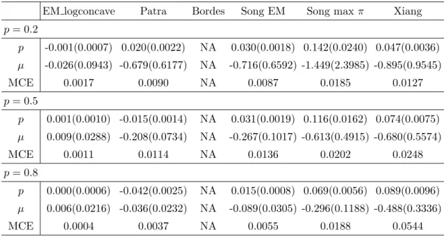
EM logconcave Patra Bordes Song EM Song max π Xiang p= 0.2 p -0.001(0.0007) 0.020(0.0022) NA 0.030(0.0018) 0.142(0.0240) 0.047(0.0036) µ -0.026(0.0943) -0.679(0.6177) NA -0.716(0.6592) -1.449(2.3985) -0.895(0.9545) MCE 0.0017 0.0090 NA 0.0087 0.0185 0.0127 p= 0.5 p 0.001(0.0010) -0.015(0.0014) NA 0.031(0.0019) 0.116(0.0162) 0.074(0.0075) µ 0.009(0.0288) -0.208(0.0734) NA -0.267(0.1017) -0.613(0.4915) -0.680(0.5574) MCE 0.0011 0.0114 NA 0.0136 0.0202 0.0248 p= 0.8 p 0.000(0.0006) -0.042(0.0025) NA 0.015(0.0008) 0.069(0.0056) 0.089(0.0096) µ 0.006(0.0216) -0.036(0.0232) NA -0.089(0.0305) -0.296(0.1188) -0.488(0.3336) MCE 0.0004 0.0037 NA 0.0055 0.0188 0.0544
Table 1.19: Bias(MSE) of estimates ofp/µ and mean of the classification error for model 5 when n= 500.
EM logconcave Patra Bordes Song EM Song max π Xiang p= 0.2 p -0.001(0.0003) 0.012(0.0011) NA 0.023(0.0009) 0.119(0.0176) 0.042(0.0025) µ -0.007(0.0438) -0.500(0.3260) NA -0.553(0.3655) 1.237(1.7273) -0.928(0.9531) MCE 0.0014 0.0058 NA 0.0061 0.0132 0.0107 p= 0.5 p -0.001(0.0006) -0.010(0.0007) NA 0.025(0.0012) 0.120(0.0179) 0.077(0.0073) µ 0.014(0.0170) -0.194(0.0565) NA -0.233(0.0722) -0.630(0.4822) -0.726(0.5840) MCE 0.0008 0.0094 NA 0.0111 0.0188 0.0240 p= 0.8 p 0.001(0.0003) -0.031(0.0013) NA 0.013(0.0004) 0.078(0.0067) 0.088(0.0087) µ 0.006(0.0094) -0.020(0.0105) NA -0.065(0.0146) -0.324(0.1188) -0.506(0.3185) MCE 0.0003 0.0026 NA 0.0039 0.0199 0.0501
Table 1.20: Bias(MSE) of estimates ofp/µ and mean of the classification error for model 6 when n= 250.
EM logconcave Patra Bordes Song EM Song max π Xiang
p= 0.2 p -0.006(0.0015) 0.003(0.0021) 0.020(0.0036) -0.012(0.0009) 0.109(0.0147) 0.027(0.0023) µ 0.127(0.1230) -0.200(0.1172) -0.685(0.8830) -0.118(0.0777) -0.654(0.5415) -0.067(0.0877) MCE 0.0464 0.0468 0.1738 0.0470 0.0509 0.0473 p= 0.5 p -0.015(0.0028) -0.044(0.0037) 0.000(0.0024) -0.045(0.0031) 0.057(0.0054) 0.031(0.0061) µ 0.073(0.0525) 0.123(0.0325) -0.009(0.0298) 0.127(0.0329) -0.099(0.0405) -0.068(0.0676) MCE 0.0688 0.0682 0.0676 0.0688 0.0683 0.0738 p= 0.8 p 0.006(0.0016) -0.077(0.0067) -0.003(0.0016) -0.059(0.0044) 0.011(0.0012) 0.006(0.0013) µ -0.024(0.0205) 0.173(0.0369) 0.004(0.0104) 0.155(0.0320) 0.032(0.0125) -0.002(0.0105) MCE 0.0591 0.0660 0.0595 0.0647 0.0588 0.0572
Table 1.21: Bias(MSE) of estimates ofp/µ and mean of the classification error for model 6 when n= 500.
EM logconcave Patra Bordes Song EM Song max π Xiang
p= 0.2 p -0.008(0.0006) -0.001(0.0008) 0.016(0.0021) -0.017(0.0007) 0.095(0.0119) 0.011(0.0007) µ 0.132(0.0565) -0.066(0.0452) -0.161(0.1613) 0.000(0.0312) -0.538(0.3834) -0.025(0.0370) MCE 0.0435 0.0457 0.0451 0.0450 0.0479 0.0439 p= 0.5 p -0.011(0.0014) -0.033(0.0019) -0.001(0.0010) -0.049(0.0030) 0.043(0.0032) 0.011(0.0017) µ 0.069(0.0304) 0.137(0.0272) -0.004(0.0109) 0.161(0.0339) -0.038(0.0183) -0.023(0.0203) MCE 0.0655 0.0676 0.0666 0.0684 0.0665 0.0664 p= 0.8 p 0.004(0.0005) -0.065(0.0047) -0.002(0.0008) -0.062(0.0043) 0.010(0.0011) 0.002(0.0007) µ -0.021(0.0069) 0.169(0.0325) -0.002(0.0054) 0.165(0.0311) 0.043(0.0102) 0.002(0.0060) MCE 0.0541 0.0646 0.0576 0.0642 0.0574 0.0546
Table 1.22: Bias(MSE) of estimates ofp/µ and mean of the classification error for model 7 when n= 250.
EM logconcave Patra Bordes Song EM Song maxπ Xiang
p= 0.2 p -0.004(0.0007) 0.016(0.0021) -0.002(0.0011) 0.025(0.0015) 0.163(0.033) 0.0273(0.0018) µ 0.011(0.0301) -0.782(0.7361) -0.043(0.0697) -0.822(0.78) -1.695(3.1805) -0.0248(0.0225) MCE 0.0133 0.0184 0.0174 0.0183 0.0338 0.0169 p= 0.5 p 0(0.001) -0.015(0.0017) 0.002(0.0011) 0.028(0.0018) 0.115(0.016) 0.0263(0.0018) µ 0.013(0.008) -0.242(0.0743) -0.008(0.0089) -0.303(0.1082) -0.63(0.4636) -0.0261(0.0083) MCE 0.0132 0.0173 0.0176 0.0189 0.0284 0.0181 p= 0.8 p -0.0080(0.0008) -0.037(0.002) -0.003(0.0008) 0.01(0.0009) 0.059(0.0043) 0.0175(0.0010) µ 0.022(0.0044) -0.03(0.0061) 0.002(0.0038) -0.102(0.0159) -0.264(0.0828) -0.0080(0.0036) MCE 0.0104 0.0106 0.0118 0.0126 0.0221 0.0144
Table 1.23: Bias(MSE) of estimates ofp/µ and mean of the classification error for model 7 when n= 500.
EM logconcave Patra Bordes Song EM Song max π Xiang
p= 0.2 p 0.000(0.0003) 0.012(0.0011) 0.000(0.0005) 0.020(0.0008) 0.173(0.038) 0.0196(0.0010) µ 0.009(0.0102) -0.566(0.3799) -0.01(0.0237) -0.625(0.4484) -1.662(3.1148) -0.0403(0.0127) MCE 0.0129 0.0157 0.0158 0.0163 0.0338 0.0156 p= 0.5 p -0.001(0.0005) -0.011(0.0009) 0.002(0.0006) 0.022(0.001) 0.121(0.0189) 0.0155(0.0007) µ 0.021(0.0038) -0.188(0.043) -0.002(0.0032) -0.243(0.0675) -0.637(0.5017) -0.0083(0.0038) MCE 0.0128 0.0155 0.0159 0.0168 0.0301 0.0159 p= 0.8 p -0.005(0.0004) -0.031(0.0014) 0.000(0.0004) 0.007(0.0004) 0.061(0.0046) 0.0129(0.0004) µ 0.02(0.0021) -0.023(0.003) -0.001(0.0017) -0.071(0.0076) -0.249(0.0748) -0.0034(0.0017) MCE 0.0101 0.0096 0.0106 0.0109 0.0204 0.0119
1.7.3 Source code
EM logconcave algorithm, R code
library(logcondens)##package for univariate log-concave density estimation library(ks)##package for Kernal density estimation
####################################### ##custom kmeans with one center fixed## ####################################### kmeans1<-function(x,center_fix){
n<-length(x) c1<-center_fix c2<-mean(x)
cluster<-numeric(n)##assign points closer to the fixed center as cluster
,→ 1 for(i in 1:n){ if(abs(x[i]-c1)<abs(x[i]-c2)){ cluster[i]<-1 }else{ cluster[i]<-2 } } c2<-mean(x[which(cluster==2)]) clusterold<-rep(1,n)
while(sum(cluster!=clusterold)!=0){ clusterold<-cluster for(i in 1:n){ if(abs(x[i]-c1)<abs(x[i]-c2)){ cluster[i]<-1 }else{ cluster[i]<-2 } } c2<-mean(x[which(cluster==2)]) } res<-list(centers=c(c1,c2),cluster=cluster,size=c(sum(cluster==1),sum( ,→ cluster==2))) return(res) } ################################################# ## EM algorithm+log concave density estimation ## #################################################
##a:density from the known component; ini_pi: true mixing proportion; ini_b
,→ : true density from the unknown component.
##using estimated initial value from kmeans true<-0 n<-length(x) fit1<-kmeans1(x,center_fix=center_known) pi<-(fit1$size[1])/n fit2<-activeSetLogCon(x=x[which(fit1$cluster==2)]) b<-evaluateLogConDens(xs=x,res=fit2)[,3] l<-sum(log(pi*a+(1-pi)*b)) lold<-l-1 while((l-lold)/abs(lold)>10^-4){ lold<-l p<-pi*a/(pi*a+(1-pi)*b)##updated probabilities pi<-sum(p)/n##updated mixing proportion
weight=(1-p)/sum(1-p) x1<-cbind(x,weight)
x1<-x1[x1[,2]>10^-4,]##delete points with weight<=10^-4 x1<-x1[order(x1[,1]),]
fit2<-activeSetLogCon(x=x1[,1],w=x1[,2]) b<-evaluateLogConDens(xs=x,res=fit2)[,3] l<-sum(log(pi*a+(1-pi)*b))
mu_loc<-sum((fit2$x)*(fit2$w))/sum(fit2$w)##use weighted sum to calculate
,→ the mean for the unknown component
res<-list(p=p,pi=pi,mu=mu_loc,x=fit2$x,phi=fit2$phi,usetrueini=true)
##use the true initial value pi1<-ini_pi b1<-ini_b l1<-sum(log(pi1*a+(1-pi1)*b1)) lold1<-l1-1 while((l1-lold1)/abs(lold1)>10^-4){ lold1<-l1 p<-pi1*a/(pi1*a+(1-pi1)*b1)##updated probabilities pi1<-sum(p)/n##updated mixing proportion
weight=(1-p)/sum(1-p) x1<-cbind(x,weight)
x1<-x1[x1[,2]>10^-4,]##delete points with weight<=10^-4 x1<-x1[order(x1[,1]),]
fit2<-activeSetLogCon(x=x1[,1],w=x1[,2]) b1<-evaluateLogConDens(xs=x,res=fit2)[,3] l1<-sum(log(pi1*a+(1-pi1)*b1))
}
if((l1>l)&&(abs((l1-l)/l)>0.0002)){ true<-1 mu_loc<-sum((fit2$x)*(fit2$w))/sum(fit2$w) res<-list(p=p,pi=pi1,mu=mu_loc,x=fit2$x,phi=fit2$phi,usetrueini=true) } return(res) }
Chapter 2
Robust Maximum Likelihood
Estimation Based on
Semiparametric Mixture Models
2.1
Introduction
Maximum likelihood estimators are widely used since they have many desirable properties such as consistency and efficiency. However, most of these estimators are very sensitive to outliers and might provide biased or even misleading results when the data are contaminated. Many robust estimators have been proposed to overcome this issue; see for example, [15], [14], [12], [13], [18], [32], [24]. However, most of the above robust estimators focus on the robust estimation of a location parameter and/or require the choice of a tuning parameter, with the exceptions of [13] and [18], which proposed a trimmed
likelihood estimation method and weighted likelihood estimation method, respectively. In this article, we propose a new class of robust maximum likelihood estimator by fitting a semiparametric mixture model to the contaminated data,
g(x) = (1−p)f0(x;θ) +pf(x), (2.1)
where f0 is a known assumed density function with unknown parameters θ ∈Θ, p∈[0,1] is the proportion of possible contaminated data/outliers, and f(x) represents the unknown density for the contaminated component. The above contaminated mixture model is com-monly used in the literature of robust statistics to describe the situation when there is violation/departure of the assumed model. Our goal is to find a robust estimation of θ
despite possible contamination from the unknown density f. By estimating the semipara-metric mixture model (2.1) directly, we can not only estimate the parameterθrobuslty but also recover the density of the contaminated component. In addition, based on the new model, we can also assign a probability of each observation being an outlier. We propose two methods to estimate the semiparametric mixture model (2.1). The first estimator is an extension of the method proposed by [21] which assumes the first component is com-pletely known without unknown parameter θ. For the second estimator, we assume that f is log-concave and then estimate the model (2.1) by maximizing the corresponding the semiparametric maximum likelihood over the unknown parameter θ and the log-concave densityf. One nice of feature of using log-concave density forf is that it can be estimated by nonparametric likelihood estimator without requiring any tuning parameter. For more details of log-concave densities, please refer to [5], [8], [34], [9] and the review of the recent
progress in log-concave density estimation by [26]. We further investigate the identifiabili-ty conditions of the proposed semiparametric mixture models and propose two innovative algorithms to estimate θ without assuming a parametric form for the contaminated densi-ty f(x). Extensive simulation studies demonstrate that our methods provide comparable performance to traditional MLE whether the data are clean and much better performance when the data contain outliers.
The rest of the paper is organized as follows. Section 2.2 discusses the identifiability problem of our model. Our two algorithms are proposed in Section 2.3. Basic theoretical properties are described in Section 2.4. In Section 2.5, we present our extensive simulation results. We conclude this article with a brief discussion in Section 2.6.
2.2
Identifiability
We first investigate the identifiability conditions of model (2.1). Without any constraints, the model (2.1) is non-identifiable. For example,
g(x) = (1−p)f0(x;θ) +pf(x) = (1−p−γ)f0(x;θ) + (p+γ)( γ p+γf0(x;θ) + p p+γf(x)), for any 0< γ <(1−p).
When f(x) represents the density of outliers, it is reasonable to assume that f(x) achieves small densities in situations where f0(x;θ) is large. If we restrict f(x) to be 0 on a fixed set, say A, with non-zero measure, then we have the following identifiable result.