Forecasting of Rice Cultivation in India–A Comparative
Analysis with ARIMA and LSTM-NN Models
Kiran Kumar Paidipati
1,*and Arjun Banik
11Department of Statistics, Pondicherry University, Puducherry-605014, India
Abstract
In India, due to the blessing by the outbreak of the National Food Security Mission, the production of cereals such as wheat, rice etc, has increased in an alarming rate. In this Study, forecasting is done with the help Auto Regressive Integrated Moving Average (ARIMA) and Long Short-Term Memory Neural Network (LSTM-NN) models on the basis of the historical data of rice cultivation from the year 1950-51 to 2017-18. The well fitted ARIMA models for the parameters such as Area under Cultivation (0,1,1), Production (0,1,1) and Yielding (2,2,1) are obtained from the significant spikes of their respective Auto Correlation Function (ACF) and Partial Auto Correlation Function (PACF) plots. But, the models fitted with a supervised deep learning neural network known as LSTM-NN are found much better time series forecasting model than the ARIMA models. The performances of these models validated with the Root Mean Square Error (RMSE) and Mean Absolute Percentage Error (MAPE) values. From the study, the LSTM-NN’s are more flexible and able to develop accurate models for predicting the behavior of agricultural parameters than the ARIMA models.
Keywords: Food Security, Rice Cultivation, ARIMA and LSTM-NN Models.
Received on 31 August 2019, accepted on 02 November 2019, published on 06 November 2019
Copyright © 2019 Kiran Kumar Paidipati and Arjun Banik licensed to EAI. This is an open access article distributed under the terms of the Creative Commons Attribution licence (http://creativecommons.org/licenses/by/3.0/), which permits unlimited use, distribution and reproduction in any medium so long as the original work is properly cited.
doi: 10.4108/eai.13-7-2018.161409
1. Introduction
Global food security is one of the major concerns in the era of twenty first century. The land under cultivation is declining drastically whereas the demand for more food is increasing at an alarming rate. There is need for serious concern to increase the food production of major food crops like rice, wheat, and maize. To improve the overall food security situation in India, there have to analyze behavior of total production along with the total area, irrigated area and productivity of these major food crops. This may create a strategic development for the future food security. The agricultural and allied industry continues to play an important role in sustainable growth and development of the Indian economy. Agriculture accounts for considerable importance in India’s economic development, as it provides food for more than 1.25 billion people.
*Corresponding Author: [email protected]
It generates employment for about 54.6% of the total population. Production of food grain covers the dominant part of the cropped area (nearly 65%) of Indian agriculture.
use allocation and environmental issues etc. Using proper statistical techniques, the parameters will get forecasted with desired precisions well in advance.
In this study, firstly ARIMA and LSTM-NN models are introduced and analysis of trends for rice cultivation under some parameters of India is done. Secondly the forecasting of rice cultivation for Area, Production and Yielding in India is done from the years 2006-07 to 2017-18 using ARIMA and LSTM-NN models and finally the comparison between these two forecasted models is done through the error analysis from the years 2013-14 to 2017-18 of Rice cultivation in India.
1.1. Review of Literature
There is much work being done with ARIMA modeling in the Agricultural Production and Yielding. Balanagammal et al. (2000) applied ARIMA models to forecast next five years for cultivable area, production, and productivity of various crops of the data during the 1956-57 to 1994-95 in Tamil Nadu. Padhan (2012) applied ARIMA models to forecast annual productivity of selected 34 different agricultural products of annual data of India from 1950 to 2010. Forecasted values have been obtained for another 5 years since 2011 and the validity of the model is verified with various model selection criteria methods. Sahu et al. (2015) analyzed the production behavior of two major crops such as Rice and Wheat of food security situation in SAARC countries through forecasting of area, production, yield and total seed production. The researchers suggested quality of seeds in good amount be made available for the farmers to produce maximum production and it will reduce the hunger and malnutrition in the region in future. Mishra et al. (2015) examined the performance of total food grains production in India and its major states during the period (1950-2009). The researchers have studied the stability in production behavior and applied ARIMA models to forecast the area, production and yield of total food grains for policy makers to achieve the food and nutrition security in India. Pushpa (2017) studied the growth of area, production and productivity of pulses for the period 1966-67 to 2015-16 through exponential growth model and applied forecasted values by ARIMA models.
Applications of Neural Networks on Agricultural Production of rice crop are very limited. Ji et al. (2007) explored precise estimation techniques to forecast the rice yields in the planning process of mountainous region in China through ANN approaches. Chaochong (2008) proposed Generalized Regression Neural Networks (GRNN) method was very much promising for prediction of grain production in rural areas. Ghosh and Koley (2014) compared the effectiveness of multiple linear regression models with ANN models with soil fertility and plant nutrition management. Sanjib (2014) explored the effects in estimating technical efficiency of rice cultivation of different agricultural farms of Odisha through various agro-climatic zones and resource allocation using the Data envelopment Analysis (DEA). The results were compared
with artificial neural networks (ANN) such as MLP and RBF to attain best possible fits to the data. Snehal et al. (2015) evaluate ANN model performance relative to variations of developmental parameters. Manjula and Djodiltachoumy (2017) explored data mining techniques based on association rules efficiently predicted crop yield estimation in Tamil Nadu region. Gandhi and Armstrong (2016 & 2017) applied data mining techniques to predict the rice yield for kharif season of humid, wet and dry subtropical climatic zones of India.
The gap is that there are no other studies concentrated on the comparison between the best fitted ARIMA model and LSTM-NN model. The focus of the study serves the purpose in forecasting the area under cultivation, production and yield of rice cultivation in India for the period of 1950-51 to 2017-18. This paper compared results of both ARIMA and ANN models and found LSTM-NN models have explored best predictions than the ARIMA models. Validity of the model was tested using standard statistical techniques. The need of the study is help for solving food security problems and also development of various policy decisions for rice crop in Eastern India.
2. Materials and Methods
2.1. Collection of Data
The data for Area under Cultivation, Agricultural Production and Agricultural Yielding of the Rice in India was collected from the Directorate of Economics and Statistics, Department of Agricultural and Cooperation, India. The dataset was partitioned from 1950 – 1951 to 2005 – 2006 was used for training the model and for model fitting and forecasting, the dataset from 2006–2007 to 2017 – 2018 for testing and validation of the fitted model.
2.2. Analysis of Trend
The dataset for area, production, and yielding of the rice in India is a time series data. These were analyzed using two trend tests i.e., (a) Mann-Kendall trend test, and (b) Cox – Stuart trend test, to detect the presence of trend in the data. These Non-parametric tests helps to analyze the data collected over time to check the constant increase or decrease in values. The data were given their ranks based on time and each of these data points are successively treated as reference data points and is compared to all the data points followed over time. Since, the data is obtained at successive time points, so the skewness and kurtosis values from the table 3.1, it is evident that the data points are non-normally distributed.
The Mann – Kendall test:-
1
1 1
(
)
n n
j i i j i
S
−sgn x
x
= = +
=
∑ ∑
−
Where,
x
iandx
jare the sequential values and the n is thelength of the dataset &
1
0
sgn ( )
0
1
1
1
if
if
if
θ
θ
θ
θ
+
>
=
=
−
<
... (2)The parameters of the Mann-Kendall test are very helpful in detecting the trend i.e., the presence of upward or downward trend and the magnitude of the trend. There are two parameters, which are useful in obtaining the strength of the trend and the magnitude of the slope.
Now, the variance of the Mann – Kendall test statistic (S) in case of ties and no ties, can be obtained as,
1
( 1)(2 5) ( )( 1)(2 5)
( ) ,
18 ( 1)(2 5) ( ) , 18 n i
i if ther
n n n t i i i
Var S
n n n
e is ties
if there is no ties Var S = − + − − + = − + =
∑
... (3) Where, ti denotes the number of ties of extent i. For large N,the test statistic is
[
]
[
]
0.5 0.51
0
var( )
0
0
1
0
var( )
sS
for S
S
Z
for S
S
for S
S
−
>
=
=
+
<
... (4)Where, Zs follows Standard Normal Distribution. Now, if
there is trend present, the magnitude of the trend can be obtained with the help of the Sen’s slope. This Sen’s slope is very much associated with the Mann-Kendall test. This can be obtained as,
,
j ix
x
Median
j i
j i
β
=
−
∀ >
−
... (5)Where, xj and xi are the two data values for the time points j
and i (j>i).
The Median of these N values of βi is known to be as Sen’s
slope estimator, such that
( 1)/2
/2 ( 2)/2
1 (
2
N
i
N N
when N isodd
Q
when N iseven
β
β
β
+ +
=
+
... (6)The value of Q indicates about the characteristics of the trend, i.e., if Q is positive, it indicates upward trend and if Q is negative, it indicates downward trend.
Now, the Cox – Stuart trend test is applicable to detect the presence of trend dependent on time, considering the observations are independent.
If X1,X2, ... Xn be the n observations, let
/ 2
(
1) / 2
n
if niseven
c
n
if nisodd
=
+
... (7)The data values are then paired as
X X
1,
1+c, ,
X X
2 2+c, ...,
X
n c−,
X
n. Then, the Cox-Stuarttest is simply a sign test on these paired data.
2.3. Model Building & Fitting
After analysing the trend in the dataset, an appropriate model is to be fitted, which will help for predicting or forecasting the future values. Here, the ARIMA and LSTM-NN models are used for fitting and the appropriate model is obtained, which fits the data more accurately with optimised error.
ARIMA Model and its notations
The ARIMA model approach for the analysis of the univariate time series data was first founded by George Box and Gwilym Jenkins. This modelling helps to predict the future values on the basis of the past values and plays a vital role in forecasting. In this study, the analysis is done through ARIMA in three stages.
Now, considering
( )
( )
t
B
tW
a
B
θ
µ
= +
Φ
... (8)Where t is the indexes time, Wt is the response series Yt, µ is
the mean term and B is the backshift operator.
The three stages are:
a) Identification Stage : In this stage, for stationarity
checking, of all the three parameters such as area, production & yielding of rice in India are found to be non-stationary, so they are converted to stationary by the method of differencing the dataset from 1950-51 to 2005-06. Then, it is used for forecasting the next 12 years i.e., 2006-07 to 2017-18. The parameters p and q of the ARIMA model were obtained with the help of significant spikes in autocorrelation and partial autocorrelation functions. In this stage, one or two model is being chosen on the basis of adequate statistical significance.
b) Estimation Stage : In this stage, the ARIMA model
is fitted and accuracy of the model is checked i.e., the error optimised model is obtained, on the basis of the following methods:
• Low AIC & BIC: Akaike's Information Criteria
(AIC) and Bayesian Information Criteria(BIC) are both useful criteria in model selection, where, AIC is estimated by
( 2log( ) 2 )
AIC
= −
L
+
m
,where, m = p+q and L is the likelihood function. Similarly, BIC can be estimated by
2log( )
log( )
BIC
= −
L m
+
n
.• Significance of autocorrelations: The
the residuals obtained should be independent of each other.
c) Forecasting Stage: In this stage, the future values
are forecasted on the basis of the past values, through the obtained model.
Artificial Neural Networks and LSTM Neural Networks
The concept of Neural Network was popularized by Hochreiter and Juergen Schmidhuber as the solution for the problem of vanishing gradient and it is developed from the concept of human neurons. The ANN and LSTM – NN lightened up the forecasting and predicting capabilities in various fields and it has very limited contribution in Agricultural field. Increase in hidden layers, increase in number of neurons, change in activation function, weight initialization etc, plays major role in improving the performance of the neural networks. In ANN, the models are firstly trained by a learning algorithm, with the help of a part of data and then, that trained model is used for testing on the left over part of data. Depending on the accuracy of the trained model, the increment or decrement of the number of neurons, the number of hidden layers is done. Among all the algorithms, back propagation is one of the important algorithms. LSTM–NN is a special type of RNN and, it is quite useful for time series forecasting. These concept of LSTM – NN is applicable in various areas and this sort of learning, includes long dependencies in data. Moreover, it is quite useful but, has a drawback in vanishing gradient. Meanwhile, this LSTM – NN cell suffers from few drawbacks, like difficulty in training a LSTM, due to the limitations in the computation of memory-bandwidth bound.
Figure 2.1. Showing the basic structure of a LSTM – NN Cell[13]
.
In the above figure of LSTM – NN cell (Figure 2.1), the gates are represented by circles. There are four types of gates gt , it , ot , and ft, each of which represents Input
Modulation Gate, Input Gate, Output Gate, and Forget Gate. The Input Modulation Gate is useful to update the current time inputs, the Input Gate and the Output Gate is useful for giving new inputs and outputs of the cell, which is to control the flow of input and output, respectively. Lastly, the Forget Gate is useful to forget some prior values, i.e., it controls the
extent to which a value remains into the cells due to some future works. All these gates, operates on the basis of current input (xt) and the previous values of states (ht-1). The
calculations for the outputs of the gates are as follows:
(
)
(
)
(
)
1 1 1t xi t hi t i
t xc t hc t c
t xf t hf t i
i
f W x W h
b
g
tanh W x
W h
b
f
f W x W h
b
− − −
=
+
+
=
+
+
=
+
+
... (9) Where, b represents the biases used in specific gate, andWx and Wh are the weights assigned for the current input and
the previous values of states. Now, the output gate can also be obtained from the current cell state, the current input and the previous state values. The updated cell state can be obtained as follows,
(
1)
t xo t ho t o
O
=
f W x W h
+
−+
b
... (10)
2.4. Evaluation of Model
The model evaluation can be performed with the help of Mean absolute Percentage Error (MAPE) and Root Mean Square Error (RMSE), which are very useful in measuring the accuracy of the fitted model.
1
/
100*
n
i i i
i
F O O
MAPE
n
=
−
=
∑
... (11) 21
(
)
n i i i
F O
RMSE
n
=−
=
∑
... (12) Where, Fi is the forecasted variable, Oi is the actual variableand n is the number of the variables. Also, the performance of the parameters depends upon the lowest MAPE value, Lowest RMSE and the Higher the R2-value.
3. Results and Discussion
3.1. Analysis of Trends
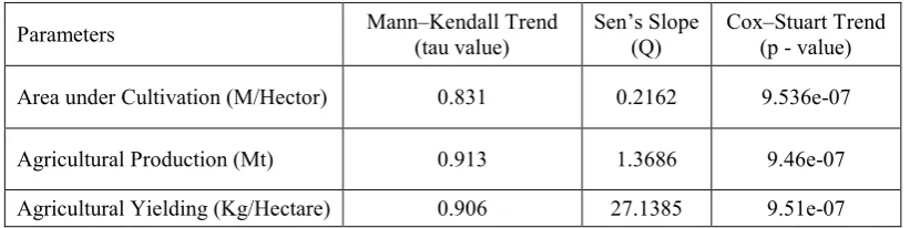
almost closer to 1 and the p–value of Cox–Stuart test is almost closer to 0, which indicates there exists trends in the data. As it is confirmed, the trend is present in these time series data, so the magnitude of the slope is obtained by the Q–value of Sen’s slope. Here, the slope of area is less as compared with other two parameters and observed high in agricultural yielding.
In the trend analysis, within all the parameters for the rice cultivation of India, it is concluded that the Q–value of the area under cultivation is low (0.216), and it results that the values are not fluctuating more about 10 years. Further it indicates the increment in the value for production and yielding, which is the only option. The results were indicated that there is a need to more focus on production
and yielding of Rice. The trend analysis has shown the increase in Q–value of the production and yielding. The Q-value for production is 1.3686, which is greater as the production increased from 20.58 Mt in 1950-51 to 112.91 Mt in 2017-18, the increment is more or less good. And the Q–value for yielding is 27.1385, as the agricultural yielding increased from 668 (kg/Hector) in 1950-51 to 2578 (kg/Hector) in 2017-18, which is much higher increment. This increment is due to the “Bringing Green Revolution in Eastern India” programme launched by the Government of India in the year 2010-11 and largely helped in increasing the production and yielding of rice cultivation in India.
Table 3.1. Showing the Descriptive Statistics of the Rice Cultivation in India (1950-51 to 2017-18)
Parameters Mean Median Standard Deviation Skewness Kurtosis
Area under Cultivation (M/Hector) 39.45 40.925 4.3877 -0.6430 -0.7593 Agricultural Production (Mt) 61.8431 57.6 27.483 0.216801 -1.345 Agricultural Yielding (Kg/Hectare) 1513.897 1437 547.0974 0.2740 -1.2725
Table 3.2. Trend Analysis with Mann – Kendall and Cox – Stuart test for the time series data of the rice cultivation in India (1950-51 to 2017-18)
Parameters Mann–Kendall Trend (tau value) Sen’s Slope (Q) Cox–Stuart Trend (p - value)
Area under Cultivation (M/Hector) 0.831 0.2162 9.536e-07
Agricultural Production (Mt) 0.913 1.3686 9.46e-07
(i) Area Under Cultivation of Rice(M/Hector) (ii) Agricultural Production of Rice(Mt)
(iii) Agricultural Yielding of Rice (Kg/ Hector)
Figure 3.1. The trends of Area under cultivation, Agricultural Production & Agricultural
Yielding of Rice in India. (1950-51 to 2017-18).
3.2 Fitting Models with ARIMA
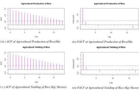
The ARIMA models are developed on the basis of the auto-regressive (p), moving average (q) and the order of differencing (d), for making the data stationary. The values of p and q are obtained with help of the significant spikes in
( i ) ACF of Area Under Cultivation of Rice(M/Hector).
(ii) PACF of Area Under Cultivation of Rice (M/Hector).
( iii ) ACF of Agricultural Production of Rice(Mt). (iv) PACF of Agricultural Production of Rice(Mt)
( v ) ACF of Agricultural Yielding of Rice (Kg/ Hector). (vi) PACF of Agricultural Yielding of Rice (Kg/ Hector).
Figure 3.2. Autocorrelation Function (ACF) and Partial Autocorrelation Function (PACF) for Area, Production and Yielding of Rice Cultivation in India (1950-51 to 2017-18)
So the best fitted model for area under cultivation is the first order moving average model with ARIMA (0, 1, 1) and it is relatively same in case of agricultural production. Agricultural yielding is second order Auto-regressive integrated moving average (ARIMA) model (2,2,1). As, in
all the cases, the ACF declines gradually and PACF has significant spike at lag 1. Then, the best fitted model is obtained on the basis of selection criterion. The model with optimised AIC and BIC value is considered as appropriately the best fitted models (See Table-3.3).
Parameters ARIMA Model AIC BIC
Area under Cultivation (M/Hector) ARIMA(0,1,1) 165.2943 171.3163 Agricultural Production (Mt) ARIMA(0,1,1) 337.2570 343.2790 Agricultural Yielding (Kg/Hectare) ARIMA(2,2,1) 662.6018 672.5467
Model building with Autoregressive Moving Average (ARIMA) Versus Long Short– Term Memory (LSTM)
The model building for the rice cultivation in India through ARIMA is good. The ARIMA models with low root mean square error (RMSE) are better, for building the appropriate model and predicting the future values. The model with low RMSE is taken, by comparing with other different ordered ARIMA models, considered to be less error for testing the
future values. The ARIMA models which gives less error in testing the predicted values with the actual values, is the final best fitted ARIMA model for the data. The obtained RMSE in the table 3.4, for ARIMA in case of Area is 0.7829, which is much less than the other models and this model gives more accurate predictions than the other ARIMA models. Similarly, in case of production and yielding of rice also observed the best fitted models with less RMSE values.
Table 3.4. Root Mean Square Error (RMSE) of ARIMA & LSTM for fitting the model for Area, Production and Yielding of Rice Cultivation in India (1950-51 to 2017-18)
Models Cultivation(M/Hector) Area Under Production(Mt) Agricultural Yielding(Kg/Hector) Agricultural
ARIMA 0.7829 5.9814 93.7801
LSTM-1 1.072 4.188 81.675
LSTM-2 0.236 3.447 65.987
Where, LSTM-1 defines the model with Batch Size: 1, Epochs: 3000, Neurons: 4
& LSTM-2 defines the model with Batch Size: 1, Epochs: 1500, Neurons: 1
Comparatively, the model building for the rice cultivation with the help of LSTM-NN, is much better than that with ARIMA. The LSTM model with single batch size is appropriate for building a best fitted model. But the difference is in the Epochs and the Neurons, the model with
Figure 3.4. ARIMA and LSTM models for the time series data of Area under Cultivation, Production and Yielding of Rice (2006-07 to 2017-18)
From the above Figure-3.4, it is concluded that the LSTM– NN with 1500 Epochs and 1 neuron is much closer to the actual values. This model can be more useful and appropriate in predicting and forecasting the future values.
3.4. Forecasting with ARIMA versus LSTM
Models
The best fitted model with ARIMA and LSTM-NN with their significant appropriate parameters is obtained and they are trained to predict the future value that is to test the forecasted values with the actual data points. From Table-5 and Table-6, the forecasted values of 5 years out of 12 years
(2006-07 to 18) that is, from the year 2013-14 to 2017-18 are shown, which are forecasted with the help of ARIMA and LSTM respectively.
Firstly, from Table-3.5, in case of ARIMA, the maximum percentage errors in forecasting are negative, which implies that the actual values are larger than the predicted values. The percentage error in forecasting 0.8737 for the year 2015-16 of the area under cultivation is the only positive value obtained, where the forecasted value is greater than the actual value, other than this, all the percentage errors in forecasting values for ARIMA are negative. Also, the errors for production varied from -8% to -2% and the yielding is from -6% to -1%.
Table 3.5. Forecasting with Autoregressive Moving Average (ARIMA) model for Area, Production and Yielding of Rice Cultivation in India for 5 Years (2013-14 to 2017-18)
Parameters Years of Forecasting Actual Values Forecasted Values Percentage error in Forecasting(±) MAPEForecasting in
Area under cultivation (M/Hector)
2013-14 2014-15 2015-16 2016-17 2017-18
43.95 43.86 43.49 43.99 43.79
43.822 43.794 43.87 43.799 43.643
-0.2912 -0.1504 0.8737 -0.4341 -0.3356
0.4171
Agricultural Production (Mt)
2013-14 2014-15 2015-16 2016-17
106.65 105.48 104.41 109.7
99.2515 100.4972 101.7428 102.9885
-6.9371 -4.7239 -2.5545 -6.118
Parameters Years of Forecasting Actual Values Forecasted Values Percentage error in Forecasting(±) MAPEForecasting in 2017-18 112.91 104.2342 -7.6838
Agricultural Yielding (Kg/Hectare) 2013-14 2014-15 2015-16 2016-17 2017-18 2424 2390 2400 2494 2578 2313.434 2343.967 2374.474 2405.614 2436.638 -4.5613 -1.926 -1.0635 -3.5439 -5.4833 3.3156
Table 3.6. Forecasting with Long Short-Term Memory ( LSTM) Model for Area, Production and Yielding of Rice Cultivation in India (2013-14 to 2017-18).
Parameters Years of Forecasting Actual Values Forecasted Values % error in Forecasting(±) MAPE in Forecasting
Area under cultivation (M/Hector) 2013-14 2014-15 2015-16 2016-17 2017-18 43.95 43.86 43.49 43.99 43.79 44.188 44.092 43.726 44.222 44.026 0.5415 0.5289 0.5426 0.5273 0.5389 0.5359 Agricultural Production (Mt) 2013-14 2014-15 2015-16 2016-17 2017-18 106.65 105.48 104.41 109.7 112.91 106.976 105.399 106.326 111.915 109.967 0.3056 -0.0767 1.8350 2.0191 -2.6065 1.3686 Agricultural Yielding (Kg/Hectare) 2013-14 2014-15 2015-16 2016-17 2017-18 2424 2390 2400 2494 2578 2330.874 2367.778 2434.358 2521.487 2527.975 -3.8418 -0.9297 1.4316 1.1021 -1.9405 1.8492
Secondly, from Table-3.6, in case of LSTM-NN, the maximum percentage errors in forecasting are positive which implies that the predicted values are larger than the actual values. The percentage errors for area are clustered around 0.5, which means the predicted values also are not fluctuating much, their deviations are more or less constant over time. For agricultural production, the percentage errors in forecasting values -0.0767 and -2.6065 for the year 2014–15 and 2017–18 are negative and it varies from -2 % to 3% and for yielding, the error varies from -4% to 2%. The deviations in LSTM are much lower than ARIMA models.
The MAPE for forecasting with the help of ARIMA model is around 6 %, but, in case of LSTM–NN , it is not even greater than 2 %, and the error in forecasting the values, with the help of LSTM–NN, is much more closer with the actual values than forecasted values with ARIMA model. So, the LSTM model with batch size 1, 1500 Epochs
and 1 neuron, resulted to be the best fitted model among all the models, under comparison of predicting the future values for the parameters such as Area under cultivation, Agricultural production and Agricultural yielding for the rice cultivation in India from 1950-51 to 2017-18.
4. Conclusions and Future Work
helps to develop more accurate models for predicting the future values than ARIMA models.
In Future, the LSTM-NN models can be applied in various agricultural fields such as sugarcane, tobacco, oilseeds etc. As, the LSTMs can learn and forecast long sequences, the LSTMs for Multi-Step forecasting can also be applicable, since they can learn to make a one shot multi-step forecast, which may also be useful for time series forecasting.
5. Limitations
This study is limited to the rice cultivation of overall India. Further, it can be extended to compare major cultivable states in India. These may give more clear pictures about how the LSTM models are better and flexible in predicting the future values.
References
[1] D. Balanagammal, C. R. Ranganathan, and R. Sundaresan (2000), Forecasting of Agricultural Scenario in Tamil Nadu-A Time Series Nadu-Analysis, Journal of the Indian Society of Agricultural Statistics, Vol. 53 (3), pp.273-286.
[2] Padhan, P.C. (2012), Application of ARIMA model for forecasting agricultural productivity in India. J. Agric. Soc. Sci., 8: 50–56.
[3] P.K. Sahu, P. Mishra, B. S. Dhekale, Vishwajith K.P., and K. Padmanaban, “Modelling and Forecasting of Area, Production, Yield and Total Seeds of Rice and Wheat in SAARC Countries and the World towards Food Security.”
American Journal of Applied Mathematics and Statistics, vol. 3, no. 1 (2015): 34-48. doi: 10.12691/ajams-3-1-7.
[4] Mishra P., et al. (2015) Study of Instability and Forecasting of Food Grain Production in India. International Journal of Agriculture Sciences, ISSN: 3710 & E-ISSN: 0975-9107, Volume 7, Issue 3, pp.-474-481.
[5] Pushpa M. Savadatti (2017), Trend and forecasting analysis of area, production and productivity of total pulses in India, Indian Journal of Economics and Development, Vol 5 (12), pp.1-10.
[6] Sanjib Kumar Hota (2014), Artificial Neural Network and Efficiency Estimation in Rice Yield, International Journal of Innovative Research in Science, Engineering and Technology, Vol. 3, Issue 7, pp. 14787-14805.
[7] B. Ji, Y. Sun, S. Yang and J. Wan (2007), Artificial Neutral Networks for Rice Yield Prediction in Mountainous Regions, Journal of Agricultural Science, Vol. 145, pp.249–261. [8] Snehal S. Dahikar, Sandeep V. Rode, Pramod Deshmukh
(2015), An Artificial Neural Network Approach for Agricultural Crop Yield Prediction Based on Various Parameters, International Journal of Advanced Research in Electronics and Communication Engineering (IJARECE) Volume 4, Issue 1, pp.94-98.
[9] E. Manjula and S. Djodiltachoumy (2017), A Model for Prediction of Crop Yield, International Journal of Computational Intelligence and Informatics, Vol. 6, No. 4, pp.298-305.
[10] Niketa Gandhi and Leisa J. Armstrong (2016), Applying data mining techniques to predict yield of rice in humid subtropical climatic zone of India, IEEE 3rd International
Conference on Computing for Sustainable Global Development (INDIACom).
[11] Niketa Gandhi and Leisa J. Armstrong (2017), Rice crop yield forecasting of tropical wet and dry climatic zone of India using data mining techniques, IEEE International Conference on Advances in Computer Applications (ICACA).
[12] Miaoguang Jin ; Chaochong Jin (2008), Forecasting Agricultural Production via Generalized Regression Neural Network, IEEE Symposium on Advanced Management of Information for Globalized Enterprises (AMIGE).
![Figure 2.1. Showing the basic structure of a LSTM – NN Cell[13].](https://thumb-us.123doks.com/thumbv2/123dok_us/8426441.1696123/4.595.54.272.471.621/figure-showing-basic-structure-lstm-nn-cell.webp)