Applications of some discrete regression
models for count data
B. M. Golam Kibria
Department of Statistics, Florida International University University Park, Miami, FL 33199, USA
Email: [email protected]
Abstract
In this paper we have considered several regression models to fit the count data that encounter in the field of Biometrical, Environmental, Social Sciences and Transportation Engineering. We have fitted Poisson (PO), Negative Binomial (NB), Zero-Inflated Poisson (ZIP) and Zero-Inflated Negative Binomial (ZINB) regression models to run-off-road (ROR) crash data which collected on arterial roads in south region (rural) of Florida State. To compare the performance of these models, we analyzed data with moderate to high percentage of zero counts. Because the variances were almost three times greater than the means, it appeared that both NB and ZINB models performed better than PO and ZIP models for the zero inflated and overdispersed count data.
Keywords: AIC; Count Data; GLM; Goodness of fit; Poisson Model; Negative Binomial; Prediction; Zero-Inflated Poisson; Zero-inflated Negative Binomial.
1. Introduction
model over Poisson or ZINB model over NB, the Vuong (1989) statistics is one of the popular test. Beside modeling crash or accidents data, these four models have been used in environmental science by Warton (2005), in biomedical science (Yau et al. 2003) among other discipline. The main objective of this paper is to provide a comprehensive review of these four models and discuss how to fit appropriate statistical models for count data using STATA software, specially for the over dispersed and an excess number of counts in the data.
The organization of this paper is as follows. The statistical methodology and goodness of fit of the models are given in section 2. To compare the performance of the models, an example has been illustrated in section 3. This paper ends up with some concluding remarks in section 4.
2. Methodology
2.1 Regression Models
In dealing with count data, for examples accident, number of ER visits, crashes that are non-negative and discrete in nature, it make more sense to model these count data using PO, NB, ZIP or ZINB distributions. Regardless of whether the assumed model is a PO, NB, ZIP or ZINB, it will be assumed that the occurrences will be independent of each other. The four types of models are described briefly in the following subsections.
2.1.1 Poisson Regression
If the variance of the counts approximately equals the mean of the count, then the Poisson regression model can be expressed as
(
)
! ) exp(
i yi i i i
i
y x
y
P = −θ θ for yi =0,1,2, (2.1) where yi is the number of counts (crashes for example) for a particular period or region i,θi is the expected number of crashes per period, which can be modeled as
), exp( β
θi = xi′
where x′i is the vector of explanatory variables and β is the vector of unknown regression parameters. The main constraint in the PO distribution is that the mean and variance are same, that is, E(Y)=V(Y)=θ. When there is a heterogeneity or over dispersion in the population, the Poisson regression does not work well. The following negative binomial (NB) regression model is a possible candidate as an alternative to PO regression.
2.1.2 Negative Binomial Model
( )
(
( )
)
yi i i i i i i i y y x y P + + Γ + Γ = αθ αθ αθ α α α 1 1 1 / 1 ! /1 1/
for yi =0,1,2,3, (2.2)
where yi is the number of crashes for road segment i,θi is the expected number of crashes per period, which can be expressed as
), exp( β
θi = x′i
The mean and variance of negative binomial distribution are respectively,
(
yi xi)
iE =θ and Var
( )
yi xi =θi[
1+θiα)]
>E(
yi xi)
. Thus the NB model is also over-dispersed and allows extra variation relative to the traditional PO model. It has more desirable properties than the Poisson model to describe the relationship between ROR crashes and geometric characteristics (Chin and Quddus 2003). The variance of NB is significantly greater than the mean. Here α represents an ancillary or dispersion parameter which indicate the degree of over dispersion. If, 0 =
α the NB regression model reduces to traditional Poisson regression model. Many researchers in different fields have considered both Poisson and Negative Binomial models: Miaou (1994), Karlaftis and Tarko (1998), Hauer (2001), Lee et al. (2002), Byers et al. (2003), Berhanu (2004), Yau et al. (2004) and Lord et al. (2005) to mention a few. However, when excess zero occur, both PO and NB regression models are not that useful to fit the zero inflated models. In that case both ZIP and ZINB models are appropriate choice.
2.1.3 Zero-Inflated Poisson (ZIP)
The zero-inflated Poisson model has a long history to use in the literature of count data to deal with an excess zeros in data. The ZIP model can be defined as
(
)
> − − = − − + = , 0 for ! ) exp( ) 1 ( 0 for ) exp( ) 1 ( i i yi i i i i i i y y y x yP θ θ
ψ
θ ψ
ψ
(2.3)
where yi is the number of crashes for road segment i, for a chosen time period, i
θ is the expected number of crashes per period, which can be modeled as
), exp( β
θi = x′i
where xi′ is the vector of explanatory variables and β is the vector of parameters, and ψ(0<ψ <1) is the probability of being in the zero crash state, determined by a logit model (Lambert 1992, Long 1997). That is
, 1 log ) ( logit
γ
ψ
ψ
ψ
e =z′i − = or , ) exp( 1 ) exp(γ
γ
ψ
i i z z ′ + ′ =i i i i ix y
E( )=θ (1−ψ )<θ and ( ) ( ).
1 1 ) ( )
( 1 i i i i
i i
i i
i x E y x E y x E y x
y
Var >
− + = ψ ψ
Thus the ZIP model is over-dispersed and allows extra variation relative to the Poisson model. If ψ =0, the ZIP model reduces to a classical Poisson regression model, otherwise the variance exceeds the mean (Long 1997). Different researchers have used ZIP model for several purposes and times, among them, Mullahy (1986), Lambart (1992), Gupta et al. (1996), Lee et al. (2001), Cheung (2002) and Yau et al. (2003) are notable. In the case of ZIP model the dual-state system exists and can be described by combining the Poisson count model (normal-count state) and the binary process (zero state) for the ZIP model. Testing for overdispersion in Poisson and binomial regression models we refer Dean (1992) among others.
2.1.4 Zero-Inflated Negative Binomial (ZINB)
The zero-inflated negative (ZINB) model can be formulated as section 2.1.3. Following Cheung (2002), the ZINB model can be expressed as
(
)
> + + Γ + Γ − = + − + = , 0 for 1 1 1 ) / 1 ( ! ) / 1 ( ) 1 ( 0 for 1 1 ) 1 ( / 1 / 1 i y i i i i i i i i i y y y y x y P i αθ αθ αθ α α ψ αθ ψ ψ α α (2.4)where yi is the number of crashes for road segment i,θi is the expected number of crashes per period, which can be modeled as
), exp( β
θi = x′i
where xi′ is the vector of explanatory variables and β is the vector of
parameters, and
ψ
is the probability of being in the zero crash state, determined by a logit model (Long 1997). That is, 1 log ) ( logit
γ
ψ
ψ
ψ
e =z′i − = or , ) exp( 1 ) exp(γ
γ
ψ
i i z z ′ + ′ =where zi′ is the vector of explanatory variables and
γ
is the corresponding vector of parameters. The mean and variance of ZINB model are respectively,i i i i ix y
E( )=θ (1−ψ )<θ and ( ) ( ).
1 1 ) ( )
( 1 i i i i
i i
i i
i x E y x E y x E y x
y Var > − + + = ψ α ψ
likelihood estimation of the parameters for ZIP or ZINB models, we refer Gupta et al. (1996), Lambert (1992), Long (1997) among others. The parameters of the models have been estimated by maximum likelihood estimation method using statistical software STATA 9.0.
2.2 Selecting Appropriate Models
2.2.1 Vuong Statistic: Selecting Inflated Model over Traditional
A number of tests for example, likelihood ratio test, the Wald test and the score tests are available for testing the zero inflation in the model (for example, see van den Broek 1995 and Lee at al., 2004 among others). For our convenience we will consider Vuong statistic, which is available in STATA. To define the Vuong (V) statistic, suppose f1
( )
yi xi and f2( )
yixi denote the probability density function of zero-inflated model (ZIP or ZINB) and parent or traditional model (PO or NB) respectively and F1( )
yi xi and F2( )
yixi denote their corresponding cumulative distribution functions. We want to test the following hypotheses0
H : Two distribution functions are equivalent a
H : Two distribution functions are different (two tailed test (two sided)) a
H : F1
( )
yixi is better than F2( )
yi xi (upper tailed test (one sided)) aH : F1
( )
yixi is worse than F2( )
yi xi (lower tailed test (one sided)) (2.5) Now we define,( )
( )
, ˆˆ log
2 1
=
i i
i i i
x y f
x y f m
where fˆ1
( )
yi xi and fˆ2(
yi xi)
are predicted probabilities of the correspondingmodels f1
( )
yi xi and f2( )
yi xi respectively. Let =∑
in= mi nm 1 1 and
∑
= −= n
i i
m m m
n
s 1 1( )2 denote the mean and standard deviation of the measurements mi. Then the Vuong statistic is defined as
n S
m V
m / =
approaches the standard normal distribution. Thus to make any decision about the null hypothesis it is reasonable to compare the observed value of the test statistic with the critical value from standard normal distribution.
2.2.2 Selecting Over Dispersed Model
To test the whether data are over dispersed or not, we test the following hypothesis,
0 : 0 α =
H
0
≠ =α a
H
The corresponding test statistic is
. ) ˆ ( ˆ
α α
SE z=
Under H0 and for large sample size, the z has approximate standard normal distribution. Reject H0 at
α
level of significance if2 /
α
Z z >
If we reject the null hypothesis we should accept that NB and ZINB models are more appropriate compare to PO and ZIP models.
2.3 Parameter Estimation and Model Selection
2.3.1 Parameter Estimation
The maximum likelihood method has been considered due to limitation of the application of STATA, which consider the maximum likelihood estimation (mle) technique. To evaluate the model, it is necessary to examine the significance of the variables included in the model. For a better model, the estimated regression coefficients have to be statistically significants. Usually, the t test is used to determine the significance of the regression coefficients. Moreover, the intuitive judgment of the experimenters should be considered.
2.3.2 Goodness of fit
After fitting some models to the data, it is essential to check the overall fit as well as quality of the fit. The quality of the fit between the observed values (y) and predicted values (µˆ) can be measured by various test statistics, however, the one of the useful statistic is called deviance and defined as:
( )
[
ˆ; ( ; )]
2 ) ˆ :
(y L y L y y
D µ =− µ −
For a better model, one would expect smaller value of the D(y:µˆ). For detailed about the fitting of a generalized linear model (GLM)s readers are refer to McCullah and Nelder (1987) and Agresti (2002) among others.
2.3.3 AIC: Selecting Best Model
, 2 2L k AIC=− +
where L is the log-likelihood and k < p is the number of parameters in the model. For the best fitted model one must expect lowest AIC value.
2.4 Model Assessment: Prediction
Our main objective is to compare the models (PO, ZIP, NB and ZINB) in the sense of better prediction. We will fit the models and then predict the number of crashes. For a better model, one would expect the predicted frequencies should be close to corresponding observed frequencies. Since the theoretical comparison is hard to make, a numerical comparison using a real data set are given in the following section.
3 Example
3.1 Data Description
the data and their properties we refer Gonzalez (2004). After fitting several models, we found that these variables are statistically significant to predict the number of crashes. We have created different data sets by deleting zero ROR crashes from 392 to 250. The summary statistics of the four set of data (number of crashes) are given in table 3.1. From the summary table it appears that all data sets are overdispersed. Thus one might expect that both NB and ZINB would possibly be better models to predict the ROR crashes.
Table 3.1: Summary Statistics
Data 250 Data 275 Data 325 Data 392
% of zero 10.0 18.2 31.0 43.0
Mean 2.33 2.12 1.79 1.48
Variance 6.66 6.50 6.08 5.49
Skewness 3.03 3.04 3.14 3.35
Kurtosis 16.28 16.55 17.62 19.58
3.2 Model Fitting
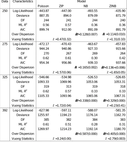
There are four sets of data and we have fitted 4 different models for each data set. To save the space of the paper, the STATA output have not provided here, however, they are available from the author upon request. The total 16 possible models and the summary of statistical analysis have been given in Table 3.2.
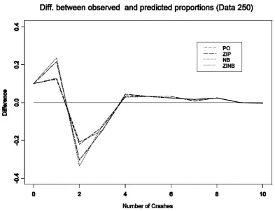
3.2.1 Model fitting to Data Set 250
Table 3.2: Summary of the fitted Models
Data Characteristics Model
Poisson ZIP NB ZINB
250 Log-Likelihood -443.87 -447.00 -493.55 -435.90
Deviance 887.35 894.0 879.09 871.79
DF 244 241 244 240
ML R2 0.56 0.57 0.36 0.36
AIC 899.74 912.00 891.09 891.79
Over Dispersion αˆ=0.128(0.007) α =0.114(0.010)
Vuong Statistics
z
=0.47(0.32)z
=1.31(0.10)275 Log-Likelihood -472.17 -470.43 -463.67 -457.83
Deviance 944.24 940.86 927.33 915.66
DF 270 267 269 264
ML R2 0.62 0.61 0.30 0.42
AIC 954.34 956.86 939.33 937.66
Over Dispersion α =0.165(0.002) αˆ =0.136=(0.006)
Vuong Statistics
z
=1.57(0.06)z
=1.65(0.05)325 Log-Likelihood -546.66 -534.98 -526.53 -526.65
Deviance 1093.33 1069.96 1053.06 1053.31
DF 319 313 319 318
ML R2 0.62 0.57 0.33 0.33
AIC 1105.33 1093.96 1065.06 1067.31
Over Dispersion αˆ=0.338(0.000) αˆ=0.329(0.000)
Vuong Statistics
z
=1.72(0.04)z
=0.23(0.41)392 Log-Likelihood -627.98 -597.11 -588.07 -581.35
Deviance 1255.97 1194.23 1176.14 1162.70
DF 385 382 384 383
ML R2 0.61 0.51 0.28 0.31
AIC 1269.97 1214.23 1192.14 1180.70
Over Dispersion αˆ=0.587(0.000) αˆ=0.405(0.000)
Vuong Statistics
z
=3.24(0.00)z
=2.79(0.003)Figure 3.1: Difference between observed and predicted proportions for number of crashes
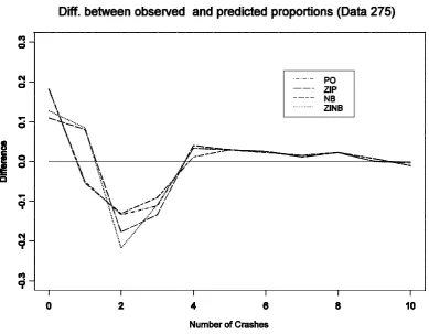
3.2.2 Model fitting to Data Set 275
Figure 3.2: Difference between observed and predicted proportions for number of crashes
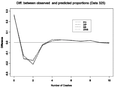
3.2.3 Model fitting to Data Set 325
Figure 3.3: Difference between observed and predicted proportions for number of crashes
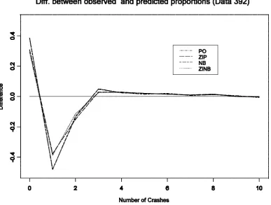
3.2.4 Model fitting to Data Set 392
figure also indicated to select ZINB model. For this data one might consider ZINB model than the ZIP model in the sense of better zero prediction.
Figure 3.4: Difference between observed and predicted proportions for number of crashes
4 Concluding Remarks
while NB models serve better while data are over dispersed. However, for an excess number of zero counts, one might consider both ZIP and ZINB regression models. It is important to note that the same set of variables or same model may not necessarily be statistically significant for another data sets with the same set of variables. For an applied research, it is advisable to fit data and then conclude based on the findings of the analysis. For a definite statement about the best fitted model, one needs more data and more analysis. Hopefully the present analysis can provides some insights to model other kind of count data, for instance, ER visit, clinical epidemiology, biometrical and environmental data.
Acknowledgments
This paper has been written based on the results of the summer 2005 project. The author is grateful to the Dean of the College of Arts and Sciences of Florida International University for providing him with summer research funding 2005. He is also thankful to the Lehman Center at FIU for using their data. The help of Javier Gonzalez with the STATA program and providing data is highly appreciated.
References
1. Agresti, A. (2002). Categorical Data Analysis. New York, Wiley.
2. Akaike, H. (1973). Information theory as an extension of the maximum likelihood principle, In the second international symposium on information theory, edited by B. V. Petrov and B. F. Csaki, Academical Kiado.
3. Berhanu, G. (2004). Models relating traffic safety with road environment and traffic flows on arterial roads in Addis Abba. Accidents Analysis and Prevention, 36, 697- 704.
4. Byers, A. L., Allore, H., Gill, T. M. and Peduzzi, P. (2003). Application of negative binomial modeling for discrete outcomes: A case study in aging research. Journal of Clinical Epidemiology, 56, 559-564.
5. Cameron, C. and Trivedi, P. (1998). Regression analysis of count data. New York: Cambridge University Press.
6. Carson, J. and Mannering, F. (2001). The effect of ice warning signs on ice-accident frequencies and severities. Accidents Analysis and Prevention, 33, 99-109.
7. Cheung, Y. B. (2002). Zero-inflated models for regression analysis of a count data: a study of growth and development. Statistics in Medicine, 21, 1481-1469. 8. Chin, H. C. and Quddus, M. A. (2003). Modeling count data with excess zeros:
An empirical application to traffic accidents. Sociological Methods and Research, 32, 90-116.
9. Dean, C. B. (1992). Testing for overdispersion in Poisson and binomial regression models. Journal of the American Statistical Association, 87, 451-457. 10. Gonzalez, J. S., Kibria, B. M. G. and Gan, A. (2005). Some discrete regression
models to determine the effects of roadway geometric features on run-off-road crashes. Submitted to Accidents Analysis and Prevention.
12. Hauer, E. (2001). Overdispersion in modeling accidents on road sections and in empirical Bayes estimation. Accidents Analysis and Prevention, 33, 799-808. 13. Javier S. Gonzalez (2004): Effects of roadway geometric features on run-off-road
crashes on the Florida State highway system. Unpublished Ph. D. thesis, Department of Civil and Environmental Engineering, Florida International University, Miami, USA.
14. Karlaftis, M. G. and Tarko, A. P. (1998). Heterogenity considerations in accident modeling. Accidents Analysis and Prevention, 30, 425-433.
15. Lambert, D. (1992). Zero-Inflated Poisson regression, with an application to defects in manufacturing. Technometrics, 34, 1-14.
16. Lawless, J. F. (1987). Negative binomial and mixed Poisson regression. Canadian Journal of Statistics, 15, 209-225.
17. Lee, A. A., Wang, K. and Yau, K. K. W. (2001). Analysis of zero-inflated Poisson data incorporating extent of exposure. Biometrical Journal, 43, 8, 963-975.
18. Lee, A. A., Xiang, L. and Fung, W. K. (2004). Sensitivity of score tests for zero-inflation in count data. Statistics in Medicine, 23, 2757-2769.
19. Lee, A. H., Stevenson, M. R., Wang, K. and Yau K. K. W. (2002). Modeling young driver motor vehicle crashes: data with extra zeros. Accidents Analysis and Prevention, 34, 515-521.
20. Lee, J. and Mannering, F. (2002). Impact of roadside features on the frequency and severity of run-off-roadway accidents: an empirical analysis. Accidents Analysis and Prevention, 34, 149-161.
21. Long, J. S. (1997). Regression Models for Categorical and Limited Dependent Variables. Thousand Oaks, CA: Sage.
22. Lord, D., Washington, S. P. and Ivan, J. N. (2005). Poisson, Poisson-gamma and zero-inflated regression models of motor vehicle crashes: balancing statistical fit and theory. Accident Analysis & Prevention, 37(1), 35-46.
23. McCullagh, P. and Nelder, J. A. (1987). Generalized linear Models, Chapman and Hall, London.
24. Miaou, S. P. (1994). The relationship between truck accidents and geometric design of road sections: Poisson versus negative binomial regressions. Accidents Analysis and Prevention, 26, 471 - 482.
25. Milton, J. and Mannering (1998). The relationship among highway geometries, traffic-related elements and motor -vehicle accident frequencies. Transportations, 25, 395-413.
26. Mullahy, J. (1986). Specifications and testing of some modified count data models. J. of Econometrics, 33 (3), 341-365.
27. Poch, M and Mannering, F. L. (1996). Negative binomial analysis of intersection accident frequency. Journal of Transportation Engineering, 122, 105-113.
28. Shankar, V., Mannering, F., and Barfield, W. (1995). Effect of roadway geometric and environmental factors on rural freeway accidents frequencies. Accidents Analysis and Prevention, 27, 371-389.
29. Shankar, V., Milton, J. and Mannering, F. (1997). Modeling accident frequencies as zero-altered probability processes: An empirical inquiry. Accidents Analysis and Prevention, 29, 829-837.
30. Stata Corporation (1999). STATA Release 9.0. College Station, Texas.
32. Vuong, Q. H. (1989). Likelihood ratio tests for model selection and non-nested hypotheses. Econometrica, 57, 307-334.
33. Warton, D. I. (2005). Many zeros does not mean zero inflation: comparing the goodness-of-fit of parametric models to multivariate abundance data. Environmetrics.
34. Wood, G. R. (2002). Generalized linear accident models and goodness of fit testing. Accident Analysis & Prevention, 34, 417-427.
35. Yau, K. K. W, Wang, K. and Lee, A. H. (2003). Zero-inflated negative binomial mixed regression modeling of over-dispersed count data with extra zeros. Biometrical Journal, 45, 437-452.