Compact and robust linear Stokes polarization camera
M. Vedel1, N. Lechocinski2, S. Breugnot3
1
Bossa Nova Technologies, Scientist R&D, CA90291, Venice, USA 2
Bossa Nova Technologies, Scientist R&D, CA90291, Venice, USA 3
Bossa Nova Technologies, Director of Operations, CA90291, Venice, USA
Abstract.We present novel applications of Bossa Nova Technologies Linear Stokes polarization camera. The SALSA camera is able to perform live measurement of Linear Stokes parameters, usual polarization parameters (Degree Of Linear Polarization and Angle Of Polarization) and other polarization based parameters (polarized image, depolarized image, virtual polarizer, polarization difference). First a brief description of the SALSA camera and its calibration is given. Then we present and discuss several results of target detection and contrast enhancement experiments. We will also introduce a novel polarization based metrological method of 3D shape measurement for in-line control of optical surfaces and control of highly aspheric optical surfaces. The architecture of the hardware and calibration results is presented. A new algorithm based on polarization imaging leading to the construction of the gradient field is described. Finally experimental results and observations as well as possible further steps are discussed.
1 Introduction
Along with intensity and spectrum polarization of light carries abundant information [1-8]. Polarization is by far the less investigated of these three fundamental properties of light. A lot of different technological approaches of imaging polarimeters have been studied [9-16]. We present in this paper the experimental results of a compact and robust polarization camera. We focused on designing both an accurate sensor and powerful software to visualize and measure in live the polarization parameters of a scene. Having access to live measurement and visualization of acquired data is the key to successful experiments, especially when these experiments are carried outdoor.
2 Polarization
imaging
Whereas standard imaging is limited to measuring the intensity of the light (which is the first Stokes parameter), polarization imaging consists in measuring at least two Stokes parameters. Polarization data contained in the Stokes parameters give much more information than a simple intensity measurement. For most of the cases, almost all the polarization information is contained in the three first Stokes parameters. Circular polarization requires specific conditions to be created (light going through a birefringent medium, light reflected by a multilayer material), so usually the last Stokes parameter contains mostly noise. Most of the current imaging
systems are so limited to analysis of the three first Stokes parameters which describe linearly polarized light.
3
Division of time polarimeters – Fast
polarization modulator
The first polarization imaging systems have been division of time polarimeters with mechanical rotation of polarizer and waveplate between frames. These systems are usually quite slow and very sensitive to motion of the scene between frames. The use of electrically driven polarization elements like liquid crystals or birefringent ceramics reduced dramatically the time required to acquire the polarization frames, allowing fast division of time polarimeters to be designed, and so limiting the registration problem caused by the motion of the scene. We developed a fast polarization modulator. It is composed of two elements. The orientation of the neutral axis of the programmable waveplates is electrically tilted by 45 degrees between the two states. Combined together, these elements give access to 4 states of polarization which are -45°, 0°, 45° and 90°. Although only three images are necessary to have linear polarization information, we chose to use the 4 images to reduce noise.
2ZQHGE\WKHDXWKRUVSXEOLVKHGE\('36FLHQFHV
4
Calibration and measurements
4.1 Calibration results
The calibration and results presented are made with a green filter (520-550nm). The Stokes parameters are linear with intensity, so the link between each pixel of the images and its Stokes parameters can be expressed with a matrix. If the images are perfectly -45°, 0°, 45° and 90° polarization, the Stokes parameters can be easily deduced, and the matrix is obviously deduced from the definition of the Stokes parameters (Erreur ! Source du
renvoi introuvable.). However the polarization states are
not perfectly -45°,0°,45° and 90°, so the C matrix is not the exactly the one in Erreur ! Source du renvoi
introuvable.. » » » » » ¼ º « « « « « ¬ ª » » » ¼ º « « « ¬ ª » » » ¼ º « « « ¬ ª o o o o 45 45 90 0 2 1 0 * 1 1 0 0 0 0 1 1 5 . 0 5 . 0 5 . 0 5 . 0 I I I I S S S (1)
Calibrating the camera consists in determining the calibration matrix that links the images acquired to the Stokes parameters. The accuracy of the calibration can be estimated by measuring degree of linear polarization (DOLP) and angle of polarization (AOP) of a rotating polarizer (Erreur ! Source du renvoi introuvable. and 3). 0 2 1 0 2 2 2 1 S iS S S S S
DOLP (2)
) ( 2 1 2 1 iS S Arg
AOP (3)
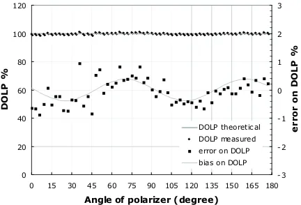
After calibration of the camera, the measurement of DOLP is excellent; the standard deviation around 100% DOLP is 0.45% (Fig. 2). It comes from a bias and from measurement noise. The bias, which is repeatable, can also be calibrated and removed. Removing this bias leads to a standard deviation of 0.35%. The measurement of AOP of the rotating polarizer is also excellent. The standard deviation of AOP is 0.15° (Fig. 22). There is no obvious bias. 0 20 40 60 80 100 120
0 15 30 45 60 75 90 105 120 135 150 165 180
Angle of polarizer (degree)
DO L P % -3 -2 -1 0 1 2 3 e r ro r on D O L P % DOLP theoretical DOLP measured error on DOLP bias on DOLP
Fig. 1. Measurement of the DOLP of a rotating polarizer. A bias of ±0.25% is observed.
0 20 40 60 80 100 120 140 160 180
0 15 30 45 60 75 90 105 120 135 150 165 180
Angle of polarizer (degree)
A O P m e a s u r ed (d e g r e e) -0.8 -0.6 -0.4 -0.2 0 0.2 0.4 0.6 0.8 1 e r r or on A O P ( d e g re e s ) theoretical angle angle measured error on AOP
Fig. 2. Measurement of the AOP of a rotating polarizer. The standard deviation is 0.15°.
4.2 Test at other DOLP
We tested if the camera was able to measure accurately DOLP other than 100%. We designed a simple experiment on which we manually rotated a dielectric surface to observe if the DOLP was following the Fresnel law. The precision of the measurement was limited by the manual rotation of the dielectric surface, the manual rotation of the illumination, and the accuracy of camera orientation. No large bias is observed and the experimental data are in excellent agreement with the theoretical prediction (figure 3). The standard deviation was measured to be only 0.017%.
0% 10% 20% 30% 40% 50% 60% 70% 80% 90% 100%
0 15 30 45 60 75 90
T (Incidence angle)
DO L P ( % ) Experimental data Theory
Fig. 3. Experimental results and theoretical predictions. No large bias is observed for DOLP lower than 100%.
5
LINEAR STOKES POLARIZATION
CAMERA
The camera (Fig.4) is a linear Stokes division of time imaging polarimeter. It uses standard CCD, standard F mount lenses, and the proprietary patented fast polarization modulator with 4 states of linear polarization. It goes up to 35 frames per seconds in full resolution and up to 111 frames per second in half resolution. The camera is compact (4”x4”x6”) and robust. The acquisition and image processing software run on a standard computer. The interface between the camera and the computer is IEEE-1394 connection (FireWire) and USB. The camera presented is integrated and can be calibrated with Red, Green, or Blue filters.
Fig. 4. Picture of the Linear Stokes camera - Field experiment with the Linear Stokes camera
6 POLARIZATION
IMAGE
PROCESSING
6.1 Raw images and Stokes parameters When the camera is calibrated, we can process the Stokes parameters to display and measure in live relevant polarization parameters. Examples are given below on a measurement. The scene observed is made of a ball, a CCD camera, and a polarizer array with all the polarizer with a different orientation. There is no polarizer in the center of the array. These objects are laid on a glass table. From the raw images acquired (Fig. 5) and the calibration matrix, the Stokes parameters can be deduced (figure 6).
Fig. 5. Raw images acquired successively: -45°, 0°, 45°, 90° linear polarization states.
Fig. 6. (a) S1 parameter = how horizontally or vertically
polarized the light is. The reflection on the glass plate is high. (b) S2 parameter = how obliquely polarized the light is
6.2 DOLP and AOP
All the polarization information is contained in the Stokes parameters but it is very difficult to interpret it. This is why more relevant parameters are computed. The most used parameters are DOLP and AOP. Figure 7 shows the DOLP image. The DOLP of all the polarizers is very high, as well as the reflections on the ball and on the
glass surface. The different orientations of the polarizers on the arrays are not distinguished.
A good way to display the AOP is to use the color hue. Color hue is a circular scale, exactly as AOP. The hue goes from red to yellow, green, blue, magenta, and finally red again. This is exactly the case of the AOP, which can be 0°, then 45°, 90°, 135°, and finally 180° which is also 0°. This way, the jump around 0° and 180° of AOP disappears with this visualization. This visualization of the AOP is much easier to understand than the display as gray values. .
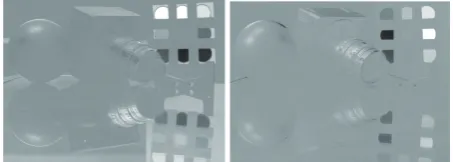
Fig. 7. (a) DOLP image coded in grayscale. (b) AOP image coded as a color HUE
6.3 Vectors overlay
Once the DOLP and AOP are known, the polarization vectors can be overlaid on any image displayed. The orientation of the vector is the AOP and the length of the vector is proportional to the DOLP (Equation. 4).
»
¼
º
«
¬
ª
)
sin(
)
cos(
AOP
AOP
DOLP
V
G
(4)The AOP and DOLP of each vector are deduced after averaging the Stokes parameters on an 11x11pixels kernel. It is very important to average the Stokes parameters which are linear in intensity and not directly the DOLP or AOP. If there is a very low signal to noise ratio, the DOLP will appear to be almost random between 0 and 1. Averaging the DOLP will lead to about 50% DOLP. Averaging the Stokes parameters and then calculating the DOLP will give the real DOLP value on the area. The signal to noise ratio on the area is 11 times better than on a single pixel.
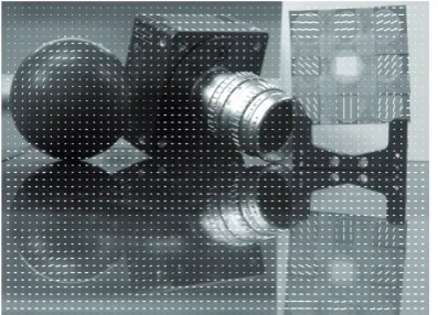
Interesting effects can be observed on the image with overlaid vectors (Fig. 9. ). For example the vectors of polarization are rotating along the ball. However on the reflection of the ball, the image is reversed but not the polarization, so they do not follow the shape of the reflection of the ball. It is also possible to calculate the normal to the surface from the DOLP and AOP data. The Fresnel equations give the link between DOLP and angle of incidence of light. Inverting this equation allows to determine the angle of incidence of light on the surface from the DOLP (Equation 5).
»
¼
º
«
¬
ª
2
sin(
2
cos(
).
(
S
S
AOP
AOP
DOLP
f
N
G
(5)a dielectric material and it does not follow the Fresnel equations if the material is not dielectric and as the calculation assumes an un-polarized environment. The material is supposed to have a 1.5 refractive index in the calculation. On the image with normal vectors overlaid, the vectors look like “hairs” on the objects (figure 9). The effect on the ball is particularly visible.
Fig. 8. Polarization vectors overlaid on intensity image
Fig. 9. Normal vectors overlaid on intensity image
6.4 Color data fusion
The most relevant color data fusion is HSL (Hue, Saturation and Luminance) color data fusion. This is essentially because hue is a circular parameter like AOP. A possible visualization is to display the intensity image and to code the polarization information only as color information (figure 10). AOP is represented as a color hue, and DOLP as the saturation of the color hue. The luminance is the real intensity of the image that makes this data fusion easy to understand as dark objects remain dark and bright objects remain bright. Color areas are associated with high DOLP areas and pale colors/grays with low DOLP areas. This visualization displays intensity and polarization information about the scene. Low DOLP areas are grey while high DOLP areas are displayed as vivid colors.
Fig. 10. Color data fusion HSL of intensity and polarization data, Hue=AOP, Saturation=DOLP, Luminance=Intensity
7
APPLICATIONS AND EXPERIMENTS
7.1 Target detection, contrast enhancement It has been showed that DOLP imaging is a powerful tool to detect man made objects [8-11]. Manmade objects are usually associated with a higher DOLP than natural objects. We tested this property with a miniature car in a scene made of random natural objects like wood and paper (Fig. 11). Whereas not obvious to detect in the intensity image, the car is the only prominent object in the DOLP image. This quick experiment shows how useful DOLP can be for automated detection and identification of manmade objects.
Fig. 11. (a) intensity and (b) DOLP image of a car in a
structured background.
As polarization information does not depend on intensity information, polarization is an excellent way to increase contrast of object. It can as well increase the contrast of object in shadows as the contrast of white object on a white background. We tested this on a white mug in a white environment (figure 12). When mapped as color, the Polarization information greatly enhanced the contrast of the mug on the background.
figure 12. (a) Intensity and (b) Color data fusion of a white mug in a white environment. The color data fusion clearly enhances the visibility of the mug on the background.
7.2 Mud detection
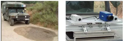
Fig. 13. (a) Ground vehicle performing tests (b) Zoom on the sensors including the presented camera.
Mud carries a strong polarization signature. The DOLP is constantly high regardless the illumination conditions. However it appeared that the DOLP of wet soil in shadow was similar of the DOLP of dry soil in shadow.
7.3 3D shape information
Polarization carries information about the 3D shape of objects [21-26]. From the normal to the surface information, the 3D shape can be reconstructed by integrating the local slopes. The first results are very promising especially for the 3D reconstruction of highly specular dielectric surfaces such as lenses. A research program is currently carried out under a National Science Foundation grant to integrate the presented camera into a new metrology system.
8 CONCLUSION
We have presented a linear Stokes polarization camera. We focused on developing both the sensor and also a powerful acquisition and processing software to have a live visualization and measurement of all the presented polarization parameters. This effective polarization camera combines:
¾ Very good calibration results ¾ Excellent sensitivity
¾ Portability and robustness for field experiments ¾ Powerful software for live polarization
measurement, analysis and visualization
Many experimental results were obtained with this camera allowed to (re)demonstrate applications of polarization imaging like target detection, contrast enhancement, 3D reconstruction, mud detection among others.
We will keep on improving software, acquiring more polarization data and conduct other experiments to find new applications for this versatile and user friendly sensor.
9 REFERENCES
1. Collett Edward, M. Dekker, Polarized Light, (1993) 2. Goldstein Dennis L., Marcel Dekker, Polarized
Light, New York, (2003)
3. Chipman E. A., M. Bass, Polarimetry, Hanbook of Optics, ed., 2, ch. 22, McGraw-Hill, New York, 2 ed., (1995).
4. Azzam R.M.A, Mueller matrix ellipsometry: a review, SPIE vol. 3121, August 1997, (1997).
5. Lu Shih-Yau & Chipman Russell A., Interpretation of Mueller matrices based on polar decomposition, J.O.S.A., Vol 13, No.5, May 1996, (1996).
6. Collot L., Breugnot S., Larive M., Volume perception by polarimetric imaging of the black-body radiations, Thomson-CSF Optronique, rue Guynemer, Automatic Target Recognition VIII, Aerosense 98, (1998)
7. Breugnot S., Le Hors L., Dolfi D. and Hartemann P., Phenomenological model of paints for multispectral polarimetric imaging, AeroSense, Orlando, (2001). 8. Goudail François, Terrier Patrick, Takakura
Yoshitate, Bigué Laurent, Galland Frédéric, De Vlaminck Vincent, Target detection with a liquid crystal-based passive Stokes polarimeter, Applied Optics, April 2003, (2003)
9. Scott Tyo J., Goldstein Dennis L., Chenault David B., and Shaw Joseph A., Review of passive imaging polarimetry for remote sensing applications, Applied Optics, Vol. 45, N22., (2006)
10. Larive M., Collot L., Breugnot S., Botma H., Roos P., Laid and flush-buried mines detection using 8-12 μm polarimetric imager, Thomson-CSF Optronique, Aerosense, (1999)
11. Clémenceau P., Breugnot S., and Collot L., Polarization diversity active imaging, Proc. SPIE 3059, 163-173 (1997)
12. Breugnot S., Clémenceau P., Modeling and performances of a polarization active imager at =806 nm, Optical Engineering, Vol.39, No. 10, 2681-2688, (2000)
13. Clémenceau P., Dogariu A., Stryjewski J., Polarization active imaging, Thomson-CSF Optronique, SPIE Aerosense, (2000)
14. Breugnot S., Le Hors L. and Hartemann P., Multispectral Polarization active imager in the visible band, AeroSense, (Orlando 2000)
15. Francia P., Bruyère F., Thiéry J.-P., Penninckx D., Simple polarization mode dispersion compensator, Electron. Lett., vol. 35, pp 414, (1999)
16. Dupont L., Sansoni T., de Bougrenet de la Tocnaye J. L., Endless smectic A* liquid crystal polarization controller, Opt. Commun., vol. 209, pp 101-106, (2002)
17. P. Nathan, S. Joseph A., Imaging spectropolarimetry of cloudy skies, Polarization: Measurement, Analysis, and Remote Sensing VII, Proceedings of the SPIE, Volume 6240, pp. 624006 (2006)
18. Coulson K. L., Polarization and Intensity of Light in the Atmosphere, Deepak Publishing, (1988)
19. Horvath G., Barta A., Gal J., Suhai B., and Haiman O., Ground-based full-sky imaging polarimetry of rapidly changing skies and its use for polarimetric cloud detection, Appl. Opt. 41, 543–559 (2002) 20. North J. and Duggin M., Stokes vector imaging of
the polarized sky-dome, Appl. Opt. 36, 723–730 (1997)
22. Atkinson Gary A., Surface Shape and Reflectance Analysis Using Polarisation, submitted for the degree of Doctor of Philosophy, (Department of Computer Science, University of York, 2007)
23. Rahmann S., Canterakis N., Reconstruction of Specular Surfaces using Polarization Imaging, Institute for Pattern Recognition and Image Processing, Computer Science Department, University of Freiburg, 79110 Freiburg, Germany. 24. Morel O., Meriaudeau F., Stolz C., Gorria P.,
Polarization Imaging Applied to 3D Reconstruction of Specular Metallic Surfaces, Le2i - CNRS UMR5158, 12 rue de La Fonderie, 71200 Le Creusot, France.
25. Morel O, Meriaudeau F, Stolz C, Gorria P, Active Lighting Applied to 3D Reconstruction of Specular Metallic Surfaces by Polarization Imaging, Le2i UMR CNRS 5158, 12 rue de la Fonderie, 71200 Le Creusot, France, Optical Society of America (2005). 26. Miyazaki D., Takashima N., Yoshida A., Harashima