Flood Frequency Analysis of Upper Krishna River Basin catchment area using Log Pearson Type III Distribution

(1)

ISSN: 2250-3021 Volume 2, Issue 8 (August 2012), PP 68-77 www.iosrjen.org

www.iosrjen.org 68 | P a g e

Flood Frequency Analysis of Upper Krishna River Basin

catchment area using Log Pearson Type III Distribution

B. K. Sathe

1

M. V. Khire

2

R. N. Sankhua

3

1

Research Scholar, CSRE, IIT-Bombay 1Corresponding author

2

Associate Professor, CSRE, IIT-Bombay,

3

Director, National Water Academy, Pune-411024

Abstract:-In this study, a flood frequency analysis of Upper Krishna River basin in India is carried out by

Log-Pearson Type-III probability distribution method. This method is a statistical technique for fitting frequency distribution data to predict the flood for a river at some site. In Upper Krishna River The annual peak flood series data for 10 years varying over period 1965 to 2010 for 7 important stations such as Karad ,Warna, Arjunwad, Kurundwad, Warungi, Terwad, Sadagli are analysed.out of these seven stations Arjunwad and Kurundwad river gauging stations are important for flash flood point of view. The probability distribution function was applied to return periods (T) of T = 2 yrs, 5yrs, 10yrs, 25yrs, 50yrs, 100yrs and 200 yrs commonly used in for engineering design of hydraulic structures. These values are useful for hydraulic design of structures in the catchment area and for storm water management .The model relates the expected discharge to return period for all tributaries of Upper Krishna River basin.

Keywords: - design discharge, flood frequency, gauge discharge, Log Person Type III, probability

I. INTRODUCTION

Floods are the most common natural disasters that affect societies around the world. Dilley et al. (2005) estimated that more than one-third of the world’s land area is flood prone affecting some 82 percent of the world’s population. About 196 million people in more than 90 countries are exposed to catastrophic flooding, and that some 170,000 deaths were associated with floods worldwide between 1980 and 2000 UNDP (2004). These figures show that flooding is a major concern in many regions of the world. To protect lives and properties it is needful for hydraulic structures to be constructed to safely handle an approximate percentage of the probable maximum flood.. As much of the hydraulic data like flow rate (discharge) and rainfall are statistical in nature, statistical methods are most frequently needed to be used often with the goal of fitting a statistical distribution to the data [11]. Design flood is the discharge adopted for the design of a hydraulic structure and it is obviously very costly to design any hydraulic structure so as to make it safe against the maximum flood possible in the catchment. [3]

The procedure for estimating the frequency of occurrence (return period) of a hydrological event such as flood is known as (flood) frequency analysis. Though the nature of most hydrological events (such as rainfall) is erratic and varies with time and space, it is commonly possible to predict return periods using various probability distributions [17]. Flood frequency analysis was developed as a statistical tool to help engineers, hydrologists, and watershed managers to deal with this uncertainty. Flood frequency is utilized to determine how often a storm of a given magnitude would occur. It is an important tool for the building and design of the safest possible structures (e.g. dams, bridges, culverts, drainage systems etc.) because the design of such structures demands knowledge of the likely floods which the structure would have to withstand during its estimated economic useful life[6].

In particular, analysis of annual one day maximum rainfall and consecutive maximum days rainfall of different return periods ( typically 2 to 100 years) is a basic tool for safe and economic planning and design of small dams, bridges, culverts, irrigation and drainage work as well as for determining drainage coefficients[4]. In this study the log Pearson Type III probability distribution function have been used to model the annual peak discharge data of Upper Krishna River Basin. The main objective of the study was to perform flood frequency analysis of the river catchment using annual peak flow or maximum discharge data obtained in the river in the water years 1965 to 2010. The specific objectives of the study were:

(i) Fit the Log Pearson Type III probability distribution to the annual peak discharge data and hence

(ii) Predict design for the following return periods (T= 2yrs, 5yrs, 10yrs, 25yrs, 50yrs, 100yrs and 200 years)

II. STUDYAREA

(2)

India. The river is 310 kms long and the catchment covers an area of 14,539 sq. km falling in Survey of India (SOI) toposheet No: 47 /K,47 /L,47 / P on 1:250,000 scale. The investigated area is enclosed between latitudes 17°18’N and 16°15′N and longitudes 73°50′E and 75°54′E. (Figure 2)

The annual peak flood series data for 10 years varying over period 1965 to 2010 for 7 important stations such as Karad ,Warna, Arjunwad, Kurundwad, Warungi of Upper Krishna basin. The data were collected from the Maharashtra state irrigation department

III. HEORY OF LOG-PEARSON TYPE IIIPROBABILITY DISTRIBUTION

The Log-Pearson Type III distribution is a statistical technique for fitting frequency distribution data to predict the design flood for a river at some site. Once the statistical information is calculated for the river site, a frequency distribution can be constructed. The probabilities of floods of various sizes can be extracted from the curve. The advantage of this particular technique is that extrapolation can be made of the values for events with return periods well beyond the observed flood events. This technique is the standard technique used by Federal Agencies in the United States.

IV. FLOOD DISCHARGE COMPUTATIONAL ANALYSIS

The Log-Pearson Type III distribution is calculated using the general equation X=𝑿+K𝝈 ( 1 )

Where k = frequency factor determined from Tables No5. The model parameters 𝑿, standard deviation and the skew coefficient (g) are computed from n observations X, with the following formula

𝑿 = 𝟏

𝒏 Xi

𝑛

𝑖=1 (2)

𝝈 = 𝟏

(𝒏−𝟏) 𝑿 − 𝑿 𝟐 𝟏/𝟐

(3)

g = 𝟏

(𝒏−𝟏) 𝑿−𝑿 𝟐

(𝒏−𝟏)(𝒏−𝟐)𝝈𝟐 (4)

However, the Log Pearson Type III distribution of X which has been widely adopted to reduce skewness is equivalent to applying Pearson Type III to the transformed variable log X and it is represented in the literature

(e.g. HannC.T.(1977) Das and Saikia (2009); Jagadesh and Jayaram (2009); Wurbs and James, 2009) as: logX=𝑙𝑜𝑔𝑋 +K𝝈logX (5)

where X is the flood discharge value of some specified probability, 𝑙𝑜𝑔𝑋 is the average of the log X discharge values, K is frequency factor. 𝝈log X is the standard deviation of log x values. The frequency factor K

is a function of skewness coefficient and return period and can be read from published tables (Table 5) developed by integrating the appropriate probability density function.The flood magnitude for various return periods are found by solving the general equation. The mean,standard deviation of the data and skewness coefficient can be calculated using the following

formula

𝑙𝑜𝑔𝑋 = log 𝑋

𝑛 (6)

𝝋𝒍𝒐𝒈𝑿=

(𝒍𝒐𝒈𝑿𝒊−𝒍𝒐𝒈𝑿)𝟐 (𝒏−𝟏)

𝟏 𝟐

(7)

g=

(𝒍𝒐𝒈𝑿𝒊− 𝑙𝑜𝑔𝑋 ) 𝟐

(𝒏−𝟏)(𝒏−𝟐)𝝈_{𝒍𝒐𝒈𝒙}𝟑 (8)

Where n is the number of entries of X the flood of some specified probability 𝑙𝑜𝑔𝑋 i is the average of the log x discharge value

V. METHODOLOGY

Log Pearson Type III distribution and given in equation 𝑻 = 𝒏+𝟎.𝟐

𝒎−𝟎.𝟒

where n is the number of years of record and m is the rank obtained by arranging the annual flood series in descending order of magnitude with the maximum being assigned the rank of 1.

(3)

(i) The annual flood series (Xii) were assembled

(ii) The logarithms of the annual flood series were calculated as yi = log Xi

(iii) The mean y, the standard deviation y and skew coefficient Cs of the logarithm yi were calculated.

(iv) The logarithms of the flood discharge i.e. log Qi for each of the several chosen probability level Pj were

calculated

using the following frequency formula

LogiQ y Kj where Kj is the frequency factor, a function of the probability Pj and Skewness coefficient

Table 5 shows the frequency factor (k) for ten selected probability levels in the range from 0.5 to 95% and skewness coefficient in the range from -3. To 3.0

(v) The flood discharge Qj for each Pi probability level (return period Tj) is obtained by taking antilogarithms of

the log𝜑 values.

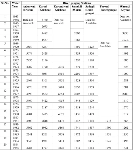
Table 1: Annual peak Discharge data for river gauging stations (m3 /s)

Sr.No. Water Year

River gauging Stations Arjunwad

(krishna)

Karad (Krishna)

Kurundwad (Krishna)

Samdoli (Warna)

Sadagli (Dudh ganga)

Terwad (Panchganga)

Warunji (Koyna)

1

1965-1966 Data not Available

4760 Data not available

Data not Available

Data not Available 2

1966-1967 2673

3

1967-1968 4482 2000 3830

4

1968-1969 1527 1068 757.4

5

1969-1970 3850 4267 1650 1225 1605

6

1970-1971 5079 2428 1555 1320 1492

7

1971-1972 2936 2156 1220 1190 1386

8

1972-1973 3989 2190 4239 1219 1230 1523

9

1973-1974 4950 3051 5659 2250 1397 1900

10

1974-1975 2469 3101 3436 1528 1304 1583

11

1975-1976 5270 3231 5781 2050 1759 1681

12

1976-1977 4890 4562 6854 2007 1103 2780

13

1977-1978 3460 3422 4953 1548 1129 1610

14

1978-1979 2579 2187 3584 1418 1244 1576

15

1979-1980 4904 2435 6070 1436 1429 1317

16

1980-1981 3800 2848 5175 1747 1103 1918 1868

17

1981-1982 3362 1942 5166 1741 1457 1790 1262

18

1982-1983 2241 1261 3438 1472 1368 1431 1156

19

1983-1984 3345 1931 5111 1682 2435 1545 1493

20

(4)

21

1985-1986 3085 1363 4414 1530 1421 1570 1054

22

1986-1987 2868 1801 4587 1347 1048 2050 1284

23

1987-1988 2351 1323 3290 1080 872.6 1392 1073

24

1988-1989 4997 3205 4870 2025 1810 2080 2590

25

1989-1990 4954 2504 6000 2412 2100 2205 1600

26

1990-1991 6500 4361 5760 1675 1452 2250 2530

27

1991-1992 5938 3150 6322 2081 1379 2553 1800

28

1992-1993 2928 2127 3919 1178 773.1 1306 1238

29

1993-1994 2843 1812 4051 1463 1058 1447 1023

30

1994-1995 6300 3915 5730 2235 1900 2680 2675

31

1995-1996 2550 1356 2796 869.0 710.9 1170 772.1

32

1996-1997 3560 2944 5000 1610 1180 1900 1566

33

1997-1998 4780 5954 6800 1710 1350 3590 3529

34

1998-1999 2411 1541 3000 897.5 685.5 1051 828

35

1999-2000 3193 2111 3725 1199 1110 1540 1397

36

2000-2001 1747 774.1 2852 1001 853.6 890.0 676.7

37

2001-2002 1764 911.2 2594 637.2 594.6 1150 623.3

38

2002-2003 1678 1121 3014 694.6 827.9 1443 830.2

39

2003-2004 1333 936.6 2275 772.1 537.7 655.0 626.7

40

2004-2005 4211 4163 4650 1261 1287 1832 2716

41

2005-2006 9381 6312 10092 3064 2200 3340 4641

42

2006-2007 7505 6708 8819 2010 1978 2797 4973

43

2007-2008 3943 3868 5673 1569 891.2 1821 2243

44

2008-2009 3357 2884 5743 1403 1013 1952 1887

Table 2 Computation of statistical parameters for Warunji (Koyna)

Rank (m)

Water Year

Qmax (X m3/s)

y = log X

(𝒚 − 𝒚)2 (𝒚 − 𝒚)3 _{T =}𝒏+𝟎.𝟐

𝒎−𝟎.𝟒 P = 𝟏𝟎𝟎

𝑻𝒓

1 _2006-2007 ₄₉₇₃ _3.6966 _0.2562 _0.1296 _70.33 _1.42

2 _2005-2006 ₄₆₄₁ _3.6666 _0.226 _0.1079 _26.37 _3.79

(5)

4 _1997-1998 ₃₅₂₉ _3.5476 _0.1275 _0.0455 _11.72 _8.53

5 _1976-1977 ₂₇₈₀ _3.4440 _0.0643 _0.0163 _9.173 _10.90

6 _2004-2005 ₂₇₁₆ _3.4339 _0.0592 _0.0144 _7.535 _13.27

7 _1994-1995 ₂₆₇₅ _3.4273 _0.0561 _0.0132 _6.39 _15.63

8 _1988-1989 ₂₅₉₀ _3.4132 _0.0496 _0.0110 _5.55 _18.00

9 1990-1991 2530 3.4031 0.0452 0.0096 4.90 20.37

10 _2007-2008 ₂₂₄₃ _3.3508 _0.0257 _0.0041 _4.39 _22.74

11 _1973-1974 ₁₉₀₀ _3.2787 _0.0077 _0.00068 _3.98 _25.11

12 _2008-2009 ₁₈₈₇ _3.2757 _0.0072 _0.0006 _3.63 _27.48

13 _1980-1981 ₁₈₆₈ _3.2713 _0.0065 _-0.0018 _3.34 _29.85

14 _1991-1992 ₁₈₀₀ _3.2552 _0.004 _0.0002 _3.10 _32.22

15 _1975-1976 ₁₆₈₁ _3.2255 _0.0012 _4.33148E-05 _2.89 _34.59 16 _1977-1978 ₁₆₁₀ _3.2068 _0.0002 _4.39277E-06 _2.70 _36.96 17 _1969-1970 ₁₆₀₅ _3.2054 _0.0002 _3.39299E-06 _2.54 _39.33 18 _1989-1990 ₁₆₀₀ _3.2041 _0.0001 _2.55537E-06 _2.39 _41.70 19 _1974-1975 ₁₅₈₃ _3.1994 _8.15857E-0 _7.36921E-07 _2.26 _44.07 20 _1978-1979 ₁₅₇₆ _3.1975 _5.05205E-05 _3.59089E-07 _2.15 _46.44 21 _1996-1997 ₁₅₆₆ _3.1947 _1.88645E-05 _8.19344E-08 _2.048 _48.81 22 _1972-1973 ₁₅₂₃ _3.1826 _6.00397E-05 _-4.6522E-07 _1.95 _51.18 23

1983-1984 1493 3.1740 0.00026

-4.40177E-06 1.86 53.55

24

1970-1971 1492 3.1737 0.00027

-4.64043E-06 1.78 55.92

25

1999-2000 1397 3.1451 0.00204

-9.26647E-05 1.71 58.29

26 _1971-1972 ₁₃₈₆ _3.1417 _0.00237 _-0.00011 _1.64 _60.66

27 _1984-1985 ₁₃₃₄ _3.1251 _0.00426 _-0.0002 _1.58 _63.033

28 _1979-1980 ₁₃₁₇ _3.1195 _0.00502 _-0.00035 _1.52 _65.40

29 _1986-1987 ₁₂₈₄ _3.1085 _0.00670 _-0.0005 _1.47 _67.77

30 _1981-1982 ₁₂₆₂ _3.1010 _0.00799 _-0.00071 _1.42 _70.14

31 _1992-1993 ₁₂₃₈ _3.0927 _0.00955 _-0.00093 _1.37 _72.51

32 _1982-1983 ₁₁₅₆ _3.0629 _0.01625 _-0.00207 _1.33 _74.88

33 _1987-1988 ₁₀₇₃ _3.0305 _0.02555 _-0.00408 _1.29 _77.25

34 _1985-1986 ₁₀₅₄ _3.0228 _0.02809 _-0.00470 _1.25 _79.62

35 _1993-1994 ₁₀₂₃ _3.0098 _0.03260 _-0.00588 _1.21 _81.99

36 _2002-2003 _830.2 _2.9191 _0.07358 _-0.01996 _1.185 _84.36

37 _1998-1999 ₈₂₈ _2.9180 _0.0742 _-0.02021 _1.153 _86.72

38 _1995-1996 _772.1 _2.8876 _0.09167 _-0.0277 _1.12 _89.09

39 _1968-1969 _757.4 _2.8793 _0.09679 _-0.03011 _1.093 _91.46 40 _2000-2001 _676.7 _2.8303 _0.12963 _-0.04667 _1.0656 _93.83

41 _2003-2004 _626.7 _2.7970 _0.15475 _-0.0608 _1.039 _96.20

42 _2001-2002 _623.3 _2.7946 _0.15661 _-0.0619 _1.014 _98.57

Average 𝑿 =1769.7 48

𝒚 =3.1

904

Sum = 2.011

Sum = 0.1250 Std. deviation

𝝈 = 𝟎. 𝟐𝟐𝟏𝟒

(6)

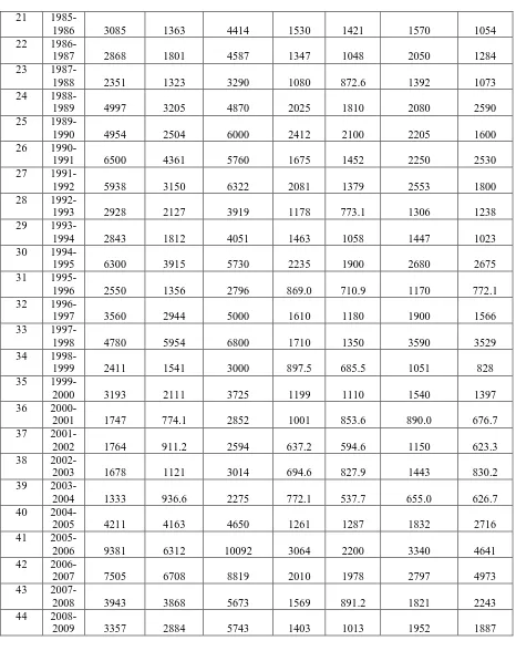
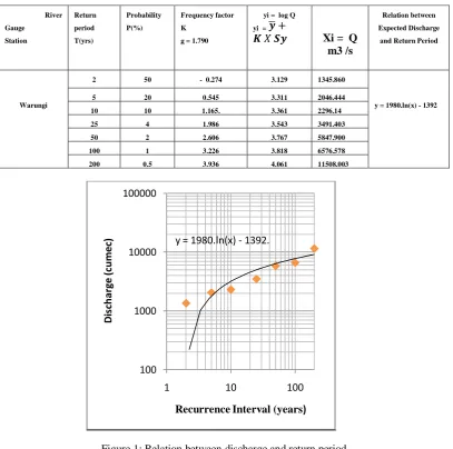
Table 3: Sample Calculation of Discharges for return periods for Warunji (Koyna)

Figure 1: Relation between discharge and return period

Table 4 Calculation of Discharges for return periods for River Gauge Stations y = 1980.ln(x) - 1392.

100 1000 10000 100000

1 10 100

D is ch arge (c u m ec )

Recurrence Interval (years)

River Gauge Station Return period T(yrs) Probability P(%) Frequency factor K

g = 1.790

yi = log Q yi = 𝒚 +

𝑲 𝑋 𝑺𝒚 Xi = Q

m3 /s

Relation between Expected Discharge

and Return Period

Warungi

2 50 - 0.274 3.129 1345.860

y = 1980.ln(x) - 1392

5 20 0.545 3.311 2046.444

10 10 1.165. 3.361 2296.14

25 4 1.986 3.543 3491.403

50 2 2.606 3.767 5847.900

100 1 3.226 3.818 6576.578

200 0.5 3.936 4.061 11508.003

Gauge Staion Frequen cy factor K Return period T(yrs)

yi = log Q yi = 𝒚 + 𝑿 𝑺𝒚

Xi = Q m3 /s Relation between Expected Discharge and

Return Period

Argunwad g = 0.2682

2 -0.029 3.558 3610

y = 1662.ln(x) + 2430.

5 0.831 3.712 5149

10 1.299 3.796 6245.8

25 1.812 3.887 7715.3

50 2.148 3.948 8864.7

100 2.457 4.003 10069

200 2.744 4.054 11333

Karad

g = 0.0112

2 -0.001 3.413 2590.5

y = 1615.ln(x) + 1405

5 0.842 3.606 4034.9

10 1.283 3.707 5088.6

25 1.754 3.814 6518.2

50 2.058 3.884 7650

100 2.332 3.946 8833.9

(7)

Kurundwa

d g = -

0.0215

2 0.081 3.675 4731.2

y = 981.4ln(x) + 4431

5 0.859 3.788 6139

10 1.221 3.841 6931.9

25 1.574 3.892 7804.1

50 1.788 3.923 8383.5

100 1.967 3.949 8901.3

200 2.120 3.972 9369.6

Sadalgi

g = - 0.4028

2 -0.048 3.295 1973.4

y = 4020.ln(x) - 2395

5 0.825 3.603 4004.8

10 1.311 3.774 5940.6

25 1.848 3.963 9186.9

50 2.208 4.090 12299

100 2.539 4.207 16096

200 2.851 4.316 20725

Samdoli

g = 1.7248

2 -0.423 3.182 1521.2

y = 5975.ln(x) - 7428

5 0.472 3.402 2521.9

10 1.257 3.595 3931.6

25 2.334 3.859 7223.6

50 3.181 4.066 11654

100 4.054 4.281 19084

200 4.934 4.497 31375

Terwad

g = - 0.3109

2 0.084 3.248 1770

y = 426.1ln(x) + 1631.

5 0.857 3.375 2369.6

10 1.215 3.433 2712.3

25 1.564 3.491 3094.3

50 1.771 3.524 3345.2

100 1.945 3.553 3571.7

(8)

Figure 2: Study area

Table 5.Frequency Factors K for Gamma and log-Pearson Type III Distributions (Haan, 1977)

Recurrence Interval In Years

1.0101 2 5 10 25 50 100 200

SKEW COEFFICIENT

Cs

Percent Chance (>=) = 1-F

99 50 20 10 4 2 1 0.5

3 -0.667 -0.396 0.420 1.180 2.278 3.152 4.051 4.970

2.9 -0.690 -0.390 0.440 1.195 2.277 3.134 4.013 4.904

2.8 -0.714 -0.384 0.460 1.210 2.275 3.114 3.973 4.847

2.7 -0.740 -0.376 0.479 1.224 2.272 3.093 3.932 4.783

2.6 -0.769 -0.368 0.499 1.238 2.267 3.071 3.889 4.718

2.5 -0.799 -0.360 0.518 1.250 2.262 3.048 3.845 4.652

2.4 -0.832 -0.351 0.537 1.262 2.256 3.023 3.800 4.584

2.3 -0.867 -0.341 0.555 1.274 2.248 2.997 3.753 4.515

2.2 -0.905 -0.330 0.574 1.284 2.240 2.970 3.705 4.444

2.1 -0.946 -0.319 0.592 1.294 2.230 2.942 3.656 4.372

2 -0.990 -0.307 0.609 1.302 2.219 2.912 3.605 4.298

1.9 -1.037 -0.294 0.627 1.310 2.207 2.881 3.553 4.223

1.8 -1.087 -0.282 0.643 1.318 2.193 2.848 3.499 4.147

1.7 -1.140 -0.268 0.660 1.324 2.179 2.815 3.444 4.069

1.6 -1.197 -0.254 0.675 1.329 2.163 2.780 3.388 3.990

1.5 -1.256 -0.240 0.690 1.333 2.146 2.743 3.330 3.910

1.4 -1.318 -0.225 0.705 1.337 2.128 2.706 3.271 3.828

1.3 -1.383 -0.210 0.719 1.339 2.108 2.666 3.211 3.745

1.2 -1.449 -0.195 0.732 1.340 2.087 2.626 3.149 3.661

1.1 -1.518 -0.180 0.745 1.341 2.066 2.585 3.087 3.575

1 -1.588 -0.164 0.758 1.340 2.043 2.542 3.022 3.489

(9)

0.8 -1.733 -0.132 0.780 1.336 1.993 2.453 2.891 3.312

0.7 -1.806 -0.116 0.790 1.333 1.967 2.407 2.824 3.223

0.6 -1.880 -0.099 0.800 1.328 1.939 2.359 2.755 3.132

0.5 -1.955 -0.083 0.808 1.323 1.910 2.311 2.686 3.041

0.4 -2.029 -0.066 0.816 1.317 1.880 2.261 2.615 2.949

0.3 -2.104 -0.050 0.824 1.309 1.849 2.211 2.544 2.856

0.2 -2.178 -0.033 0.830 1.301 1.818 2.159 2.472 2.763

0.1 -2.252 -0.017 0.836 1.292 1.785 2.107 2.400 2.67

0 -2.326 0.000 0.842 1.282 1.751 2.054 2.326 2.576

-0.1 -2.4 0.017 0.846 1.27 1.716 2.000 2.252 2.482

-0.2 -2.472 0.033 0.850 1.258 1.680 1.945 2.178 2.388

-0.3 -2.544 0.050 0.853 1.245 1.643 1.890 2.104 2.294

-0.4 -2.615 0.066 0.855 1.231 1.606 1.834 2.029 2.201

-0.5 -2.686 0.083 0.856 1.216 1.567 1.777 1.955 2.108

-0.6 -2.755 0.099 0.857 1.200 1.528 1.720 1.880 2.016

-0.7 -2.824 0.116 0.857 1.183 1.488 1.663 1.806 1.926

-0.8 -2.891 0.132 0.856 1.166 1.448 1.606 1.733 1.837

-0.9 -2.957 0.148 0.854 1.147 1.407 1.549 1.660 1.749

-1 -3.022 0.164 0.852 1.128 1.366 1.492 1.588 1.664

-1.1 -3.087 0.180 0.848 1.107 1.324 1.435 1.518 1.581

-1.2 -3.149 0.195 0.844 1.086 1.282 1.379 1.449 1.501

-1.3 -3.211 0.210 0.838 1.064 1.240 1.324 1.383 1.424

-1.4 -3.271 0.225 0.832 1.041 1.198 1.270 1.318 1.351

-1.5 -3.33 0.240 0.825 1.018 1.157 1.217 1.256 1.282

-1.6 -3.880 0.254 0.817 0.994 1.116 1.166 1.197 1.216

-1.7 -3.444 0.268 0.808 0.970 1.075 1.116 1.140 1.155

-1.8 -3.499 0.282 0.799 0.945 1.035 1.069 1.087 1.097

-1.9 -3.553 0.294 0.788 0.920 0.996 1.023 1.037 1.044

-2 -3.605 0.307 0.777 0.895 0.959 0.980 0.990 0.995

-2.1 -3.656 0.319 0.765 0.869 0.923 0.939 0.946 0.949

-2.2 -3.705 0.330 0.752 0.844 0.888 0.900 0.905 0.907

-2.3 -3.753 0.341 0.739 0.819 0.855 0.864 0.867 0.869

-2.4 -3.800 0.351 0.725 0.795 0.823 0.830 0.832 0.833

-2.5 -3.845 0.360 0.711 0.711 0.793 0.798 0.799 0.800

-2.6 -3.899 0.368 0.696 0.747 0.764 0.768 0.769 0.769

-2.7 -3.932 0.376 0.681 0.724 0.738 0.740 0.740 0.741

-2.8 -3.973 0.384 0.666 0.702 0.712 0.714 0.714 0.714

-2.9 -4.013 0.390 0.651 0.681 0.683 0.689 0.690 0.690

(10)

VI. CONCLUSIONS

Flood frequency analysis is one of the most challenging problems in hydrology. The hydrologic phenomena are often characterized by great variability and uncertainty precipitation, discharge. For this reason, a systematic approach to handling the problem is absolutely essential.

From the flood frequency study carried out on Upper Krishna River basin catchment for 2 yrs, 5yrs, 10yrs, 25yrs, 50yrs, 100yrs and 200 yrs The estimated discharges obtained . It has been observed that design floods for return period of 2 year were flood to be almost same as the observed data and verified with historical data. Arjunwad river gauging station is having very high design flood as compare to other gauging station in the study area. These flood frequencies and design can be used as a guide in determining the capacity and design of structure like bridges, culverts.

ACKNOWLEDGEMENT

The author is pleased to acknowledge to Chief Er.C.A.Birajdhar and H.T.Dhumal, Department of Water recourse, Govt .of Maharashtra for availability of data and encouragement to write this paper.Greatful acknowledgement are also due to Prof. Nayan Sharma, Professor &Head Department of WRD&M, and Prof. Pradeep Kumar Garg, Indian Institute of Technology,Roorkee who reviewed and given insightful comments on drafting of this paper.

REFERENCES

[1] Akintola, J.O. 1986 Rainfall distribution in Nigeria 1892-1983, Impact publishers Nig. Ltd., Ibadan.

[2] Arora, K.R. 2007. Irrigation, Water Power and Water resources Engineering. Standard Publishers Distributors, New Delhi [3] Asawa, G.L. 2005. Irrigation and Water resources Engineering. New Age International Ltd. Publishers,New Delhi

[4] Bhakar, S.R., Bansal, A.N. Chhajed, N., and Purohit, R.C. 2006. Frequency analysis of consecutive days maximum rainfall at Banswara, Rajasthan, India. ARPN Journal of Engineering and Applied Sciences. 1(3): 64-67.

[5] Borbda and Benin Owena 2005.River basin Hydrological year Book, 1995-1998

[6] Bruce, J.P., and Clark, P.H. 1988. Introduction to hydrometeorology. Pergamon Press, Oxford

[7] Chow, V.T., D.R.Maidment and L.W.Mays 1988. Applied Hydrology. McGraw Hill Book Company,Singapore.

[8] Garg P.K., K.P.Sharma.and S.C.Jain.1986 Satellite Remote Sensing for Mapping of Flood-Plains and Allied Features, Int. Symp. on Flood Frequency and Risk Analysis, Louisiana, USA.

[9] Haktan Y.T 1992. Comparison of Various flood frequency distribution using annual flood peaks data of rivers in Anatolis. Journal of Hydrology. Vol.136; pp1-31

[10] Haan, C.T. 1977. Statistical methods in hydrology. Ames, IA: Iowa State University Press.

[11] Ibrahim M.H., and E.A. Isiguzo, 2009. Flood Frequency Analysis of Guara River Catchment at Jere, Kaduna State, Nigeria,. Scientific Research and Essay Vol. 4 (6), pp. 636 – 646.

[12] Jagadesh, T.R. and M.A.Jayaram 2009. Design of bridge Structures. 2nd Edition. PHI Learning PVT Ltd, New Delhi India [13] Prasuhn, A. 1992. Fundamentals of Hydraulic Engineering. Oxford University Press New York

[14] O.C.Izinyon,N.Ihimkpen. Flood Frequency Analysis of Ikpoba River Catchment at Benin city Using Log Prearson Type III [15] Distribution, Journal of Emerging Trends in Engineering and Applied Sciences Vol.2(1) pp-50-55

[16] Ojha, G.S.P.,R Berndtsson .and P.Bhunya 2008. Engineering Hydrology. 1st Edition, Oxford University Press. New Delhi, India [17] Sankhua, R.N.N. Sharma, P.K.Garg, and A.D.Pandey, 2005. Use of remote sensing and ANN in assessment of erosion activities in

Majuli, the world’s largest river island: Int. Journal of Remote Sensing, Vol. 26, pp. 4445 – 4454.