A graph clustering algorithm based on a clustering coefficient for weighted graphs

DOI 10.1007/s13173-010-0027-x O R I G I N A L PA P E R

A graph clustering algorithm based on a clustering coefficient

for weighted graphs

Mariá C.V. Nascimento·André C.P.L.F. Carvalho

Received: 27 May 2010 / Accepted: 29 November 2010 / Published online: 21 December 2010 © The Brazilian Computer Society 2010

Abstract Graph clustering is an important issue for several applications associated with data analysis in graphs. How-ever, the discovery of groups of highly connected nodes that can represent clusters is not an easy task. Many assump-tions like the number of clusters and if the clusters are or not balanced, may need to be made before the application of a clustering algorithm. Moreover, without previous infor-mation regarding data label, there is no guarantee that the partition found by a clustering algorithm automatically ex-tracts the relevant information present in the data. This pa-per proposes a new graph clustering algorithm that automat-ically defines the number of clusters based on a clustering tendency connectivity-based validation measure, also pro-posed in the paper. According to the computational results, the new algorithm is able to efficiently find graph clustering partitions for complete graphs.

Keywords Clustering coefficient·Graph clustering· Combinatorial optimization

1 Introduction

Data clustering deals with the discovery of data patterns, in the form of data clusters, in the objects from a dataset. For such, objects with similar characteristics are placed into the same group (cluster) and objects with different features are

M.C.V. Nascimento (

e-mail:mariah@icmc.usp.br

A.C.P.L.F. Carvalho e-mail:andre@icmc.usp.br

placed into different clusters. Several clustering algorithms have been proposed in the literature, based on several ap-proaches. These algorithms have been successfully applied to a wide variety of problems, including applications from areas like bioinformatics [11], image processing [25] and market segmentation [2]. Despite the good results obtained by the use of clustering algorithms in several problem do-mains, cluster analysis is still seen as a challenging problem. Some particular clustering problems require more sophisti-cated algorithms.

A specific problem of clustering is known as graph clus-tering. Graph clustering looks for patterns among nodes in a graph in order to produce a meaningful node partitioning. Many inferences about the node partition may provide use-ful information regarding the data. A few examples of the benefits, as well as different approaches for graph cluster-ing, can be found in [24].

Additionally, in spite of the large number of clustering algorithms, few of them are able to automatically discover partitions without the information of the number of clusters beforehand. Automatic graph clustering algorithms, able to define by themselves the number of clusters, play an im-portant role in data analysis, since they allow a more effi-cient application of clustering algorithms to a dataset with-out prior knowledge of the data conformation. Therefore, the investigation of new clustering algorithms able to deal with graph clustering problems and to automatically define the number of clusters is an important research issue.

be-tween the presence of an edge connecting a pair of nodes from a same cluster and the probability that the same edge can be found at the same cluster in a random graph. The lower this probability, the higher the measure value. Thus, the best value is the highest value that can be achieved.

A measure frequently used to evaluate the clustering ten-dency of the nodes of a graph is the clustering coefficient measure [30]. The clustering coefficient of a node measures how much its neighbors are close to a clique, i.e., a com-plete subgraph. This measure assesses the number of trian-gles around a node divided by its number of possible cliques. In this paper, we propose a new validation measure based on the clustering coefficient. As a result of the optimiza-tion of this measure, we introduce an algorithm in order to find graph clustering partitions with the maximum proposed clustering coefficient. This algorithm does not require the previous definition of the number of clusters in the partition. Computational experiments were carried out and the results obtained indicate a very good potential for finding good par-titions using the proposed algorithm.

The rest of this paper is organized as follows. Section2 presents the proposed measure based on clustering coeffi-cient. In Sect. 3, a new clustering algorithm based on the optimization of the proposed measure is presented. Sec-tion4describes another measure, modularity, used in a com-parison with the proposed measure. Finally, in Sect. 5 we evaluate the new measure and the quality of the partitions found by the introduced clustering algorithm. For such, we perform some experiments with several datasets. To sum up, Sect.6presents the main conclusions derived from the analysis of the experimental results.

2 Assessment measure

LetG=(V , E)be a graph whereV andEare, respectively, its set of nodes and edges. The number of nodes ofGisn. Each edge is represented by a pair(i, j ), whereiandj are nodes from V. In this paper, the nodes are represented by natural numbers from 1 ton.

Consider A= [aij]n×n to be the adjacency matrix of graph G. Each element of the adjacency matrix has a bi-nary value, representing the relationship between two nodes. Thus,aij=1 if nodesiandjare adjacent, i.e., if there is an edge linking nodeito nodej, andaij=0 otherwise.

This paper deals with weighted graphs. LetW= [wij]n×n be the weight matrix for the edges of a weighted graphG. The elementwij of this matrixW is defined as the weight of the edge that links nodei to nodej. If there is no edge between a pair of nodesiandj, thenwij=0.

The degree of a node i, degi, from an unweighted or weighted graph, is calculated considering the number of its

adjacent objects. It is given by (1).

degi= n

j=1

aij. (1)

A measure that evaluates the clustering tendency in graphs is known asclustering coefficient [30]. It is based on the analysis of three node cycles around a nodei. A for-mulation of this measure for unweighted graphs is given by (2).

Ci=

2n_j−₌1_1kn_=j+1aijaj kaik degi(degi−1)

(2)

Note that n_j−₌₁1 j=i

n k=j+1

k=i

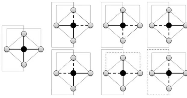
aijaj kaik corresponds to the number of triangles around node i. The degreedeg_i indi-cates the total number of neighbors of nodei. The denomi-nator measures the maximum possible number of edges that could exist between the vertices within the neighborhood. This measure evaluates the tendency of the nearest neigh-bors of nodei to be connected to each other [20], as illus-trated by Fig.1.

This figure presents a subgraph (the first left-handed pic-ture with no dashed lines) with a central black-colored node iand its four adjacent nodes (gray-colored). This means that the degree ofiis 4 (the number of its incident edges high-lighted by solid black lines). The maximum number of edges between the neighbors ofiis 6, which is 4×3/2, as can be noticed in this picture. The number of triangles around the nodeiis also 6 (as shown in the 6 subgraphs with dashed lines), meaning that the clustering coefficient of this partic-ular nodeiis 1.

According to [20], to extend this measure to weighted graphs, it is necessary to replace the part of the numerator, that indicates the number of triangles around nodei, by the sum of the triangles intensities around nodei. The formula-tion presented by the authors is:

Ci(W )=

2n_j−₌1₁n_k=j+1(w˜ijw˜ikw˜j k)1/3 degi(degi−1)

, (3)

Fig. 1 Illustration of the clustering coefficient measure

Based on this weighted clustering coefficient, we propose a validation measure able to analyze the cluster tendency of a partition. For such, consider the following equation:

di= n

j=1

aijxij, (4)

wherexij is a binary variable that assumes value 1, if the nodesiandj belong to the same cluster, and 0, otherwise. It must be observed thatdi is the number of nodes adjacent toiand that belong to the cluster with nodei. The proposed clustering coefficient of a node i from a partition π of a weighted graph is given by the following equation:

Cci(π )=

2n_j−₌1₁n_k=j+1(w˜ijw˜j kw˜ik)1/3 di(di−1)

yij k, (5)

whereyij k is a binary variable that assumes value 1 if the nodesi,j andkbelong to the same cluster and 0, otherwise. In this paper, we propose a solution method (heuristic) based on the optimization of the introduced clustering coef-ficient index. No proof with respect to the complexity of the problem whose goal is to detect the partition with the max-imum proposed index is provided in this paper. In spite of this, according to our knowledge, no polynomial algorithm is always able to find such partition. Moreover, it is well known that the complexity of a variety of graph partitioning problems is NP-hard [6].

3 Solution method

Multilevel clustering algorithms are a special class of graph clustering algorithms that have been extensively used to find high quality clustering solutions. Some of these algorithms can be found in [4,12,13]. They are known for having three different phases: coarsening, partitioning, andrefinement. The first phase, coarsening phase, compresses a graph by contracting its nodes. The second phase, partitioning phase,

partitions the graph found in the coarsening phase. The last phase, refinement phase, expands the partitioned graph un-til it reaches its original structure by the simultaneous im-provement of the current solution by the application of some method, like a local search.

In this paper, we propose a simple multilevel clustering algorithm. Its phases work as follows:

1. Coarsening phase: A sequence of matching’s among the graph edges is performed until the graph reaches a pre-defined size.

2. Partitioning phase: In this phase, the coarsened graph is partitioned by the multi-level algorithm METIS [12,13]. Many other partitioning algorithms, such as spectral clus-tering algorithms, were tested. However, METIS pro-duced better results in a shorter time.

3. Refinement phase: The partition found in the previous phase is improved by a local search after each step of the expansion of the graph nodes by reverting the coars-ening. This process continues until the original structure of the graph is obtained.

Details of each phase of the algorithm are presented next.

3.1 Coarsening phase

The coarsening phase consists in performing matching’s of the edges from a graph. A matching on a graphG is de-fined by a setSof edges where, for every(i, j )∈S, there is no edge(k, j ), withk=ior(k, i)withk=j that belongs toS. The maximum matching problem looks for a matching whose set of edges has the maximum total weight.

For such, the edge weights between nodei(and nodej) and all its adjacent nodes have now to take into account the edge weights between these adjacent nodes with the other node in the matching, nodej (and nodei). An usual way to calcu-late the edge weight between a nodeiand one of its adjacent nodes,k, is summing up the edge weights connectingiwith kandj withk.

In this paper, the coarsening phase is performed until the number of nodes becomes lower than or equal to the maxi-mum value between 100 and 0.2n. If a graph already has a number of nodes lower than or equal to 100, one iteration of the matching is performed. This final coarsened graph, named base graph, is partitioned in the next phase of the multilevel algorithm. The partitioning of this base graph is detailed in the next section.

3.2 Partitioning phase

According to multilevel algorithms, after the graph is coars-ened, it is partitioned by a partitioning algorithm. In this pa-per, we applied a multilevel partitioning algorithm named METIS [12]. Other algorithms were tested, but METIS pre-sented better final partitions.

As METIS requires the number of clusters to be defined a priori, we find partitions using METIS for{2, . . . ,20} clus-ters.

As a result, we have 19 different initial partitions to be refined. After the refinement phase, the partition with the best proposed clustering coefficient is returned as the final partition of the algorithm.

3.3 Refinement phase

In this phase, a local search procedure is applied to every partition found in the partitioning phase. Many different lo-cal search procedures were evaluated. We chose the lolo-cal search with the best combination of efficiency and perfor-mance. For such, consider

ti= n−1

j=1

n

k=j+1

(w˜ijw˜ikw˜j k)1/3

di(di−1) yij k.

Local Search (Solution)

Step 0: Read the graph and its partition to be refined by the local search. Makeit←0.

Step 1: Unmark all nodes.

Step 2: Choose an unmarked node i whose ti is lower thant_i.t_iis calculated in the same way asti, chang-ing the solution variables as if nodeibelonged to a clusterc, different from where it belongs to. Mark nodei. Ifn <500, go to Step 3, else, go to Step 4. Step 3: If moving node i to cluster cimprove the current

solution, go to Step 4. Else, go to Step 5. Step 4: Move nodeito clusterc.

Step 5: If all nodes are marked, makeit←it+1 and go to Step 6, else, go to Step 2.

Step 6: If there was no improvement in this iteration orit> 100, then go to Step 7. Else, go to Step 1.

Step 7: Return the most updated solution.

If the graph has more than 500 nodes, we eliminate Step 3, which is very expensive. However, when the graph has less than 500 nodes, it is viable to perform Step 3. This local search allows the number of clusters to change from the initial partition, when this produces a better solution.

As the order of the nodes to perform the matchings is random, different coarsened graphs can be achieved by the coarsening phase. For this reason, we perform all steps of the proposed multilevel algorithm 10 times. Only the best solution among these 10 runs is kept.

In summary, the proposed multilevel clustering algorithm (MLA-CC) has the following steps.

Multilevel algorithm (G) Step 0: ReadG. Makeit←0.

Step 1: (Coarsening phase) Contract graphGas it was pre-sented in the coarsening phase section.

Step 2: (Partitioning the base graph) Find the 19 partitions by METIS, as it was explained in Sect.3.2.

Step 3: (Refinement phase) Apply the local search pre-sented in Sect.3.3at each of the 19 partitions found in the previous step. Keep the best solution found.

Step 4: (Update solution) Ifit=0 or the solution found in the previous step is higher than the overall best solution, then the overall best solution is updated by the best solu-tion found in the previous step. Makeit←it+1. Step 5: Ifit>10 then go to Step 6, else, go to Step 1. Step 6: Return the best solution.

Next, a validation graph clustering measure extensively used in the last years will be presented. Partitions found by algorithms based on the optimization of this measure will be used to compare with the results of our algorithm.

4 Modularity index

The modularity index was proposed in [19]. It measures the clustering tendency of a graph partition, considering its probability in the same partition in a random graph with the same node degree sequence. To see how it works, letπ be a partition from a graphG. Consider the following equation:

q(π )= 1 2m

n

i=1

n

j=1 rijxij.

IfGis a weighted graph, 2m=n_l=1n_k=1wlk, andrij defined by the following equation:

rij=wij−

n k=1wik

n k=1wj k

n l=1

n k=1wlk

Heuristics based on the search of the partition with max-imum modularity have been extensively proposed in litera-ture [3]. Due to the quality of the partitions found by these algorithms, they are largely used as the main references for graph clustering.

5 Computational experiments

In order to analyze the performance of the proposed algo-rithm, we performed two sets of experiments: the first with artificial graphs and the second with real datasets converted into similarity graphs. Each one of the experiments is ex-plained in the next sections. In these experiments, we com-pare our heuristic with the following graph clustering al-gorithms from the literature: a spin glass-based algorithm (Spinglass) [23], a fast greedy modularity-based algorithm (FastGreedy) [3] and a walktrap algorithm (Walktrap) [21]. They were all proposed for graph clustering problems and do not require the definition of the number of clusters. We used their implementation from the R-project [29] in the package igraph. All of them use the validation measure adopted by the authors, the modularity measure (the parti-tion with the best modularity in the iteraparti-tions of the algo-rithms is always chosen). The comparison of the algoalgo-rithms is based on the real classification of the datasets. For such, we use the Adjusted Rand Index(ARI), proposed in [10]. This index allows to compare the similarity between the par-tition found by an algorithm for a given dataset with the real classes. The value for this index is better when its value is higher. The minimum and maximum values achieved by this measure are, respectively,−1 and 1.

5.1 First experiment

In order to analyze the behavior of the proposed solution method, MLA-CC, experiments were carried out with sixty artificial modular graphs, generated using the function Sim-DataAffiliation from the package Statistical Inference for Modular Networks(SIMoNe). The parameters used to gen-erate the graphs were set in order to make them highly mod-ular. We generated six graphs for each of the following num-ber of nodes: 100, 200, 300, 400, 500, 600, 700, 800, 900, and 1000. For each number of nodes, there is one graph with 2, 3, 4, 5, 10, and 20 modules (clusters in the structure of the graph).

As a result of this experiment, we observed that the pro-posed algorithm presented ARI values worse than the other algorithms used in the comparison. The analysis of these re-sults showed that, in general, a poor performance of MLA-CC was observed when the input graph was not complete. Additional experiments were then carried out using com-plete graphs. In these new experiments, our algorithm per-formed better than the other algorithms used in the compar-ison. These results suggest that a transformation of a non

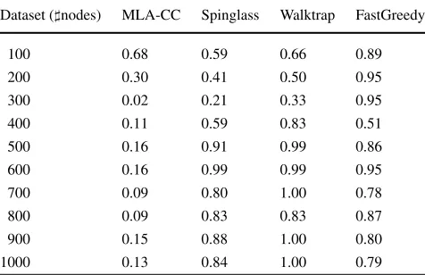
Table 1 Average ARI values of the partitions found by the algorithms regarding the clustering labels provided by the data generator. Each average corresponds to the mean ARI of the partitions for all artificial graphs with the same number of nodes

Dataset (nodes) MLA-CC Spinglass Walktrap FastGreedy

100 0.68 0.59 0.66 0.89

200 0.30 0.41 0.50 0.95

300 0.02 0.21 0.33 0.95

400 0.11 0.59 0.83 0.51

500 0.16 0.91 0.99 0.86

600 0.16 0.99 0.99 0.95

700 0.09 0.80 1.00 0.78

800 0.09 0.83 0.83 0.87

900 0.15 0.88 1.00 0.80

1000 0.13 0.84 1.00 0.79

complete graph into a complete graph could improve the performance of the proposed algorithm in the other datasets. However, this transformation may not be efficient, since to work with a sparse matrix is, in general, computationally easier than with non sparse matrices. We tested a conversion of non complete graphs to a complete graph version using an approach based on the pairwise shortest paths between the nodes. Even though the proposed algorithm achieved bet-ter results with these converted graphs than with the orig-inal noncomplete graphs, the performance of the resulting algorithm was inferior to the performance observed in the other evaluated algorithms. Table1shows these results (us-ing graphs transformed to complete graphs by a shortest path approach for MLA-CC and raw graphs for the other algo-rithms).

The results from Table1 show that the proposed algo-rithm has ARI values similar to the other algoalgo-rithms only for the smallest number of nodes. Its performance becomes significantly worse than the other algorithms with the in-crease of the number of nodes. These results suggest that the proposed algorithm should not be used in noncomplete graphs. However, additional experiments using real datasets indicated a niche where the proposed algorithm has a very good potential. These experiments are presented in the next section.

5.2 Second experiment

In this second experiment, fourteen real datasets were used. Eleven of them are biological datasets and three are bench-mark datasets largely used in cluster analysis. The main as-pects of these datasets are explained in Tables2and3.

Table 2 Table of the description of the biological datasets used in the second experiment

Golub[8] is a dataset with 3,571 gene expression levels of 47 tissues of acute lymphocyte leukemia (ALL) samples and 25 tissue samples of acute myeloid leukemia (AML). ALL may be classified in 2 classes: B-lineage with 38 samples and T-lineage with 9 samples

BreastA[28] andBreastB[31] are datasets with, respectively, 98 and 48 samples, of breast tumor generated using one-channel oligonucleotide and two-channel microarrays. The version employed is pre-processed with 1,213 attributes each. Regarding the classification, in [9] can be observed an analysis ofBreastAdividing it in 3 classes with 11, 51, and 36 samples.BreastB, like in [18], was decomposed into 2 classes regarding the estrogen receptor (ER). In this dataset, there are 25 samples of positive ER (ER+) 24 samples of negative (ER−). The collection of tumors consists of 13 samples of ER+lymph node (LN)+tumors, 12 samples of ER−LN+tumors, 12 samples of ER+LN−tumors, and 12 samples of ER−LN−tumors

DLBCLC[26] is a dataset with 58 samples of patients with Diffuse large B cell lymphoma (DLBCL). Its number of attributes is 3,795, which corresponds to a preprocessed version from [9]. The classes of this dataset correspond to the cured DLBCLs (32 samples) and the fatal/refractory tumors (26 samples)

Leukemia[32]: This dataset has 327 samples with 271 gene expression levels. It can be classified into 7 classes: BCR-ABL (15 samples), E2A-PBX1 (27 samples), Hiperdiploid>50 (64 samples), MLL (20 samples), T-ALL (43 samples), TEL-AML1 (79 samples) and others (79 samples). An alternative grouping divides the example in 3 more general subgroups, in which the first includes B-ALL, which consists of samples BCR, E2A, TEL, and MLL; the second is composed of T-ALL; and last one consists of “others” type

Lung[1]: This dataset consists of 197 lung tumor samples with 1,000 gene expression levels. Its classification into 4 types of cancer includes 139 samples of adenocarcinomas, 21 samples of carcinomas from squamous cells and 20 samples of carcinoids. A pre-processed version from [16] was used

MultiA[27] is a preprocessed cancer tissue dataset [9]. It has the same examples and classes asNovartis, except for the number of attributes, which is higher, 5565

MultiB[22] is, as well asMultiA, a cancer tissue dataset. It is also a pre-processed version found in [9] and has 32 samples with 5,565 attributes. This dataset has 4 classes corresponding to different types of tissues: 5 breast tissues, 9 prostate tissues, 7 lung tissues and 11 colon tissues

Novartis[16,27]: This dataset has 1,000 gene expression levels from 103 cancer tissue samples. The classification comes from their origin: 26 from breast, 26 from prostate, 28 from lung and 23 from colon

MiRNA[14]: This dataset corresponds to 218 mammal tissue samples of human and tumor origins with gene expression profiles of 217

microRNAs. The samples are classified into 20 classes with 6, 15, 10, 11, 3, 9, 18, 7, 19, 10, 8, 5, 14, 2, 26, 28, 8, 8, 3 and 8 samples according to their origin

Yeast[17] is a 8 attribute dataset with 1484 yeast proteins samples. As it can be observed in [17], the dataset can be classified into 10 classes regarding the localization site of proteins, with 463, 429, 244, 163, 51, 44, 37, 30, 20, and 5 objects

Table 3 This table shows the description of the non-biological datasets used in the experiments

Glass[5] is a classical 9 attribute dataset of criminal investigation scenes with 214 samples. The samples may be divided into 6 classes according to the physic chemical properties, with 70, 76, 17, 13, 9 and 29 examples

Iris[7] is a 4 classical attribute dataset with 150 examples of 3 species of the Iris flower: 150 samples of Iris setosa, 150 samples of Iris virginica and 150 samples of Iris versicolor

Simulated6[16] is an artificial dataset with 60 samples with 600 genes as attributes. This dataset can be divided into 6 classes with 8, 12, 10, 15, 5 and 10 samples. Each class is defined by 50 distinct genes, which are uniquely regulated for each class

edges linking pairs of nodes are weighted according to the weight matrixW. The weights are calculated according to the Euclidean distance, using (8).

wij=1− dij dmax

, (8)

wheredij is the Euclidean distance between objectsi and j, and dmax is the maximum distance between any pair of objects from the dataset. Other ways for constructing a graph from a dataset could be used. However, many studies, like

[15], claim that the discovery of the most suitable way to represent a dataset in a graph is not an easy task. Therefore, for simplicity, in this paper, we just used this strategy for constructing graphs from datasets.

5.2.1 Results of the second experiment

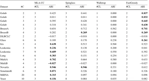
Table 4 ARI values of the partitions found by the algorithms. The best ARI for each dataset is highlighted in bold

MLA-CC Spinglass Walktrap FastGreedy

Dataset #C #CL ARI #CL ARI #CL ARI #CL ARI

Golub 2 3 0.425 3 0.441 1 0.000 2 0.837

Golub 2 3 0.011 3 0.011 1 0.000 2 0.032

Golub 3 3 0.395 3 0.428 1 0.000 2 0.645

Golub 4 3 0.318 3 0.341 1 0.000 2 0.630

BreastA 3 2 0.654 3 0.712 3 0.562 2 0.741

BreastB 4 3 0.202 2 0.269 1 0.000 2 0.269

DLBCLC 2 2 −0.017 2 −0.018 1 0.000 2 −0.018

Glass 6 6 0.189 3 0.170 3 0.238 2 0.261

Iris 3 4 0.638 3 0.513 2 0.568 2 0.523

Leukemia 3 9 0.236 5 0.138 4 0.200 3 0.041

Leukemia 7 9 0.689 5 0.521 4 0.550 3 0.392

Lung 4 6 0.303 3 0.151 3 0.254 2 0.117

MultiA 4 5 0.702 3 0.664 3 0.580 3 0.633

MultiB 4 2 −0.027 2 −0.027 1 0.000 2 −0.027

Novartis 4 4 0.946 4 0.946 2 0.331 3 0.612

Simulated6 6 5 0.871 3 0.326 2 0.180 3 0.326

MiRNA 20 8 0.315 2 0.097 2 0.094 2 0.098

Yeast 10 3 0.156 8 0.084 2 0.035 2 0.082

clusters of the partitions found by the indicated algorithm. These results are concerned with the real classification of the datasets provided in literature.

As can be seen on Table4, according to the ARI mea-sure, MLA-CC found the best ARI more times than the other algorithms. In the cases where one of the other al-gorithms obtained better results than MLA-CC, their ARI values were very close (except for the datasetGolub). There-fore, considering these datasets, the proposed graph cluster-ing algorithm for weighted graphs produced good results. Moreover, it can be noticed that the majority of the results, for all algorithms, were lower than 0.4. This fact suggests that in many cases the dataset had not a clear clustering structure, or that it is not easily identified. Taking as ex-ample the dataset MiRNA, one may observe that the par-titions found by the other algorithms have a very low re-semblance with the real classification of the dataset (since their ARI values were around 0.098). The partition found by MLA-CC for this same dataset has a much better suit-ability to the real data classification (in this case, the ARI was 0.315, more than three times higher than the other algo-rithms). Another dataset for which the proposed algorithm achieved much better results, when compared with the other algorithms, was the datasetSimulated6. On the other hand, for the datasetGolub, the FastGreedy algorithm found a par-tition with a much better average ARI value than the other algorithms.

Table 5 Table of objective

function values Dataset CC

Golub 0.590159

BreastA 0.78431

BreastB 0.575682

DLBCLC 0.630128

Glass 0.793655

Iris 0.839137

Leukemia 0.642047

Lung 0.687603

MultiA 0.490546

MultiB 0.598776

Novartis 0.543799

Simulated6 0.685092

MiRNA 0.715988

Yeast 0.776264

Regarding the computational efficiency of the proposed heuristic, there is a significant impact of both the number of natural clusters and the number of nodes in the dataset on the computational time. In general, the lower the num-ber of natural clusters, the higher the computational time. Although there is no clear pattern associating the number of clusters and the computational time, we estimate an increase of 10% in running time for each cluster (e.g., a dataset with 3 clusters and 100 nodes took 4 seconds, whereas the running time for a dataset with the same number of nodes and 2 clus-ters was about 4.5 seconds). There is also a large impact of the number of nodes on the computational time necessary to find the solution (although we can make no assertion about its relation to the number of nodes, it is approximately twice the solution time for a dataset with one hundred less nodes). In comparison with the other algorithms, MLA-CC took ap-proximately the same time as Spinglass to find the parti-tions (both took the largest computational times among all tested algorithms, about ten times slower than FastGreedy and Walktrap).

6 Final remarks

This paper presented a novel graph clustering algorithm based on a well-studied measure known as clustering coef-ficient. The measure consists in the analysis of the connec-tivity of a node regarding the connecconnec-tivity of its neighbors

and is commonly used to measure the clustering tendency of the nodes in a graph. In this paper, a variation of an exist-ing weighted version for clusterexist-ing coefficient is proposed in order to evaluate the quality of the partitions of weighted graphs. Using this variation, an algorithm based on the opti-mization of the proposed measure is presented.

In order to validate the quality of the proposed algorithm, we compared its results with the results of other graph clus-tering algorithms from literature. The comparison was based on a measure that evaluates the fitness of a pair of partitions (the partitions found by algorithms and the real classifica-tion of the data). In a first experiment with artificial modular graphs, we observed a poor performance of the proposed al-gorithm, with much worse results than from the literature for noncomplete graphs. By studying the behavior of the results of our algorithm, we discovered that it worked better when the case study was a complete graph. Then, in a second ex-periment with complete graphs, we attested that the parti-tions found by the proposed algorithm had a better quality if compared with the partitions obtained with algorithms from literature considering the classification of the real datasets. Therefore, the proposed algorithm for weighted graphs is a valuable novel contribution for graph clustering for com-plete graphs.

Acknowledgements The authors gratefully acknowledge FAPESP, CAPES, and CNPq for their financial support.

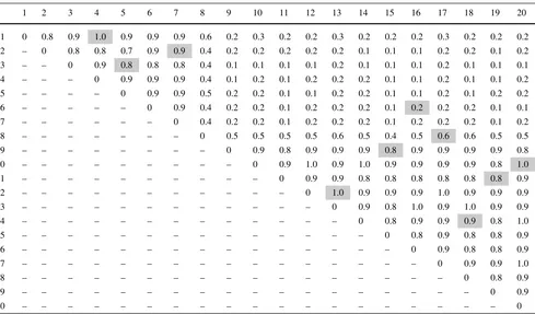
Table 6 Weight matrix of the toy example, where the matching of the coarsening phase is represented by the edges highlighted by gray boxes

1 2 3 4 5 6 7 8 9 10 11 12 13 14 15 16 17 18 19 20

1 0 0.8 0.9 1.0 0.9 0.9 0.9 0.6 0.2 0.3 0.2 0.2 0.3 0.2 0.2 0.2 0.3 0.2 0.2 0.2

2 – 0 0.8 0.8 0.7 0.9 0.9 0.4 0.2 0.2 0.2 0.2 0.2 0.1 0.1 0.1 0.2 0.2 0.1 0.2

3 – – 0 0.9 0.8 0.8 0.8 0.4 0.1 0.1 0.1 0.1 0.2 0.1 0.1 0.1 0.2 0.1 0.1 0.1

4 – – – 0 0.9 0.9 0.9 0.4 0.1 0.2 0.1 0.2 0.2 0.2 0.1 0.1 0.2 0.1 0.1 0.2

5 – – – – 0 0.9 0.9 0.5 0.2 0.2 0.1 0.1 0.2 0.2 0.1 0.1 0.2 0.1 0.2 0.2

6 – – – – – 0 0.9 0.4 0.2 0.2 0.1 0.2 0.2 0.2 0.1 0.2 0.2 0.2 0.1 0.1

7 – – – – – – 0 0.4 0.2 0.2 0.1 0.2 0.2 0.2 0.1 0.2 0.2 0.2 0.1 0.2

8 – – – – – – – 0 0.5 0.5 0.5 0.5 0.6 0.5 0.4 0.5 0.6 0.6 0.5 0.5

9 – – – – – – – – 0 0.9 0.8 0.9 0.9 0.9 0.8 0.9 0.9 0.9 0.9 0.8

10 – – – – – – – – – 0 0.9 1.0 0.9 1.0 0.9 0.9 0.9 0.9 0.8 1.0

11 – – – – – – – – – – 0 0.9 0.9 0.8 0.8 0.8 0.8 0.8 0.8 0.9

12 – – – – – – – – – – – 0 1.0 0.9 0.9 0.9 1.0 0.9 0.9 0.9

13 – – – – – – – – – – – – 0 0.9 0.8 1.0 0.9 1.0 0.9 0.9

14 – – – – – – – – – – – – – 0 0.8 0.9 0.9 0.9 0.8 1.0

15 – – – – – – – – – – – – – – 0 0.8 0.9 0.8 0.8 0.9

16 – – – – – – – – – – – – – – – 0 0.9 0.8 0.8 0.9

17 – – – – – – – – – – – – – – – – 0 0.9 0.9 1.0

18 – – – – – – – – – – – – – – – – – 0 0.8 0.9

19 – – – – – – – – – – – – – – – – – – 0 0.9

Table 7 The pairwise weight matrix of the coarsened graph from the example

[12,13] [20,10] [2,7] [8,17] [11,19] [14,18] [4,1] [15,9] [16,6] [3,5]

[12,13] 0 1.11 0.13 0.89 1.08 1.12 0.14 1.07 0.65 0.10

[20,10] – 0 0.15 0.86 1.04 1.13 0.16 1.03 0.61 0.09

[2,7] – – 0 0.27 0.08 0.12 1.04 0.08 0.56 0.95

[8,17] – – – 0 0.77 0.83 0.34 0.79 0.53 0.28

[11,19] – – – – 0 0.99 0.06 0.99 0.49 0.06

[14,18] – – – – – 0 0.14 1.03 0.57 0.03

[4,1] – – – – – – 0 0.08 0.58 1.09

[15,9] – – – – – – – 0 0.55 0.05

[16,6] – – – – – – – – 0 0.51

[3,5] – – – – – – – – – 0

Appendix: a running example

This Appendix presents one iteration of a toy example of MLA-CC with a small dataset. In this example, we used the first 20 objects of the datasetSimulated6. Each step of the algorithm is presented in the next sections.

7.1 Coarsening phase

As we are dealing with a complete graph example, let us rep-resent its weighted edges on a weight matrix. The resulting matching between the nodes of this example is represented in the weight matrix illustrated in Table6by the gray boxes. According to Table 6, the edge between nodes 4 and 1 is matched, since the box corresponding to the first row and forth column is marked by the gray color. In Table7, the node of the coarsened graph corresponding to the matching of this edge is referred as [4,1]. Thus, one has a graph with 10 nodes (resulted from the coarsening of the original graph by the matching) whose weighted edges are showed in Ta-ble7(calculated as explained before).

7.2 Partitioning phase

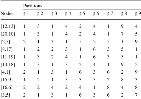
The coarsened graph is then partitioned at this phase of the algorithm. In this paper, we used a strategy that generates partitions from 2 to 10 clusters using METIS (for a larger dataset, it would be possible to generate 2 to 19 clusters, as presented in the algorithm description). The resulting parti-tions are presented in the matrix in Table 8, where theith row represents the node i from the coarsened graph, and each number of the matrix is the class label of the result-ing partition (represented in each column). Usresult-ing these 9 partitions, the refinement phase of the proposed algorithm is performed.

7.3 Refinement phase

In this phase of the algorithm, at each uncoarsening step (in this example, it is just one step, due to the small size of the

Table 8 Table with the partitions found by METIS for the coarsened graph

Partitions

Nodes 1 2 3 4 5 6 7 8 9

[12,13] 1 3 1 4 2 4 1 9 4

[20,10] 1 3 1 4 2 4 1 7 5

[2,7] 2 1 3 1 5 2 5 1 9

[8,17] 1 2 2 3 1 6 3 5 1

[11,19] 1 3 2 4 1 6 3 5 1

[14,18] 1 3 1 3 2 4 1 9 5

[4,1] 2 1 3 1 6 3 6 2 9

[15,9] 1 2 1 5 3 5 2 8 3

[16,6] 2 2 4 2 4 1 8 4 8

[3,5] 2 1 3 1 6 3 6 2 7

dataset), a local search is applied to the current partition. For each of the 9 partitions, the uncoarsening of the coarsened graph followed by a local search is performed (updating the labels). For example, in the forth partition of the coarsened graph, the first row corresponds to the first node of the coars-ened graph that corresponds to the nodes 12 and 13 of the original graph (indicated as [12,13]). Both of them will re-ceive the label 1, as indicated in Table9.

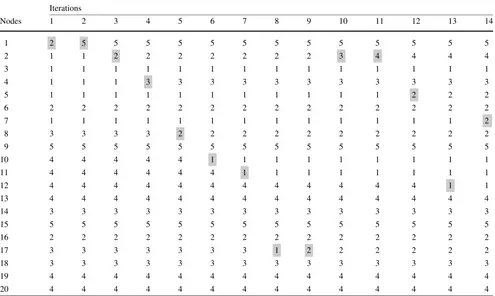
At this phase, the local search is applied to the partition of the current iteration. As already described, the local search consists in the transfer of nodes between the clusters in the partition of a graph in such a way that the transfer produces a partition with a better clustering coefficient-based index. The refinement phase of the forth partition (the one that pro-duces the solution with best proposed index in the end of the procedure) is summarized in Table10.

Table 9 This table shows the uncoarsened partition number four

Nodes 1 2 3 4 5 6 7 8 9 10 11 12 13 14 15 16 17 18 19 20

Label 1 1 1 1 1 2 1 3 5 4 4 4 4 3 5 2 3 3 4 4

Table 10 The partitions found at each of the 14 iterations of the local search from the refinement phase of MLA-CC. The movements of the local search are highlighted by gray boxes

Iterations

Nodes 1 2 3 4 5 6 7 8 9 10 11 12 13 14

1 2 5 5 5 5 5 5 5 5 5 5 5 5 5

2 1 1 2 2 2 2 2 2 2 3 4 4 4 4

3 1 1 1 1 1 1 1 1 1 1 1 1 1 1

4 1 1 1 3 3 3 3 3 3 3 3 3 3 3

5 1 1 1 1 1 1 1 1 1 1 1 2 2 2

6 2 2 2 2 2 2 2 2 2 2 2 2 2 2

7 1 1 1 1 1 1 1 1 1 1 1 1 1 2

8 3 3 3 3 2 2 2 2 2 2 2 2 2 2

9 5 5 5 5 5 5 5 5 5 5 5 5 5 5

10 4 4 4 4 4 1 1 1 1 1 1 1 1 1

11 4 4 4 4 4 4 1 1 1 1 1 1 1 1

12 4 4 4 4 4 4 4 4 4 4 4 4 1 1

13 4 4 4 4 4 4 4 4 4 4 4 4 4 4

14 3 3 3 3 3 3 3 3 3 3 3 3 3 3

15 5 5 5 5 5 5 5 5 5 5 5 5 5 5

16 2 2 2 2 2 2 2 2 2 2 2 2 2 2

17 3 3 3 3 3 3 3 1 2 2 2 2 2 2

18 3 3 3 3 3 3 3 3 3 3 3 3 3 3

19 4 4 4 4 4 4 4 4 4 4 4 4 4 4

20 4 4 4 4 4 4 4 4 4 4 4 4 4 4

References

1. Bhattacharjee A, Richards WG, Staunton J, Li C, Monti S, Vasa P, Ladd C, Beheshti J, Bueno R, Gillette M, Loda M, Weber G, Mark EJ, Lander ES, Wong W, Johnson BE, Golub TR, Sugarbaker DJ, Meyerson M (2001) Classification of human lung carcinomas by mRNA expression profiling reveals distinct adenocarcinoma sub-classes. Proc Natl Acad Sci USA 98(24):13790–13795

2. Boginski V, Butenko S, Pardalos PM (2006) Mining market data: a network approach. Comput Oper Res 33:3171–3184

3. Clauset A, Newman MEJ, Moore C (2004) Finding community structure in very large networks. Phys Rev E 70(6):066111 4. Dhillon IS, Guan Y, Kulis B (2007) Weighted graph cuts

with-out eigenvectors a multilevel approach. IEEE Trans Pattern Anal Mach Intell 29(11):1944–1957

5. Evett IW, Spiehler EJ (1987) Rule induction in forensic science. In: KBS in government, online publications, pp 107–118 6. Feder T, Hell P, Klein S, Motwani R (1999) Complexity of graph

partition problems. In: 31ST ANNUAL ACM STOC. Plenum, New York, pp 464–472

7. Fisher RA (1936) The use of multiple measurements in taxonomic problems. Ann Eugen 7:179–188

8. Golub TR, Slonim DK, Tamayo P, Huard C, Gaasenbeek M, Mesirov JP, Coller H, Loh ML, Downing JR, Caligiuri MA,

Bloomfield CD, Lander ES (1999) Molecular classification of can-cer: class discovery and class prediction by gene expression mon-itoring. Science 286(5439):531–537

9. Hoshida Y, Brunet JP, Tamayo P, Golub TR, Mesiro JP (2007) Subclass mapping: identifying common subtypes in independent disease data sets. PLoS ONE 2(11):e1195

10. Hubert L, Arabie P (1985) Comparing partitions. J Classif 2:193– 218

11. Huttenhower C, Flamholz AI, Landis JN, Sahi S, Myers CL, Ol-szewski KL, Hibbs MA, Siemers NO, Troyanskaya OG, Coller HA (2007) Nearest neighbor networks: clustering expression data based on gene neighborhoods. BMC Bioinform 8:250

12. Karypis G, Kumar V (1996) Parallel multilevel graph partition-ing. In: Proceedings of the international parallel processing sym-posium

13. Karypis G, Kumar V (1998) A fast and high quality multilevel scheme for partitioning irregular graphs. SIAM J Sci Comput 20(1):359–392

14. Lu J, Getz G, Miska EA, Alvarez-Saavedra E, Lamb J, Peck D, Sweet-Cordero A, Ebert BL, Mak RH, Ferrando AA, Downing JR, Jacks T, Horvitz RR, Golub TR (2005) Microrna expression profiles classify human cancers. Nature 435(7043):834–838 15. Maier M, von Luxburg U, Hein M (2009) Influence of graph

infor-mation processing systems, vol 21, pp 1025–1032. Curran, Red Hook

16. Monti S, Tamayo P, Mesirov J, Golub T (2003) Consensus clus-tering: a resampling-based method for class discovery and visu-alization of gene expression microarray data. Kluwer Academic, Dordrecht. Tech rep, Broad Institute/MIT

17. Nakai K, Kanehisa M (1991) Expert system for predicting protein localization sites in gram-negative bacteria. Proteins 11:95–110 18. Nascimento MCV, Toledo FMB, Carvalho ACPLF (2010)

Inves-tigation of a new GRASP-based clustering algorithm applied to biological data. Comput Oper Res 37:1381–1388

19. Newman MEJ, Girvan M (2004) Finding and evaluating commu-nity structure in networks. Phys Rev E 69:026113

20. Onnela JP, Saramäki J, Kertész J, Kaski K (2005) Intensity and coherence of motifs in weighted complex networks. Phys Rev E 71:065(R), 103(R)

21. Pons P, Latapy M (2005) Computing communities in large networks using random walks. In: Computer and information sciences—ISCIS 2005, pp 284–293

22. Ramaswamy S, Tamayo P, Rifkin R, Mukherjee S, Yeang CH, An-gelo M, Ladd C, Reich M, Latulippe E, Mesirov JP, Poggio T, Gerald W, Loda M, Lander ES, Golub TR (2001) Multiclass can-cer diagnosis using tumor gene expression signatures. Proc Natl Acad Sci USA 98(26):15,149–15,154

23. Reichardt J, Bornholdt S (2006) Statistical mechanics of commu-nity detection. Phys Rev E 74:016 110

24. Schaeffer SE (2007) Graph clustering. Comput Sci Rev 1:27–64 25. Shi J, Malik J (2000) Normalized cuts and image segmentation.

IEEE Trans Pattern Anal Mach Intell 22:888–905

26. Shipp MA, Ross KN, Tamayo P, Weng AP, Kutok JL, Aguiar RCT, Gaasenbeek M, Angelo M, Reich M, Pinkus GS, Ray TS, Koval

MA, Last KW, Norton A, Lister TA, Mesirov J (2002) Diffuse large b-cell lymphoma outcome prediction by gene-expression profiling and supervised machine learning. Nat Med 8:68–74 27. Su AI, Cooke MP, Ching KA, Hakak Y, Walker JR, Wiltshire

T, Orth AP, Vega RG, Sapinoso LM, Moqrich A, Patapoutian A, Hampton GM, Schultz PG, Hogenesch JB (2002) Large-scale analysis of the human and mouse transcriptomes. Proc Natl Acad Sci USA 99:4465–4470

28. van ’t Veer LJ, Dai H, van de Vijver MJ, He YD, Hart AA, Mao M, Peterse HL, van der Kooy K, Marton MJ, Witteveen AT, Schreiber GJ, Kerkhoven RM, Roberts C, Linsley PS, Bernards R, Friend SH (2002) Gene expression profiling predicts clinical outcome of breast cancer. Nature 415(6871):530–536

29. Venables WN, Smith DM (2010) An introduction to R. R Devel-opment Core Team, The R Foundation for Statistical Computing, version 2.11.1

30. Watts D, Strogatz S (1998) Collective dynamics of small-world networks. Nature 393:440

31. West M, Blanchette C, Dressman H, Huang E, Ishida S, Spang R, Zuzan H, Olson JA, Marks JR, Nevins JR (2001) Predicting the clinical status of human breast cancer by using gene expression profiles. Proc Natl Acad Sci USA 98(20):11462–11467