ISSN (Online): 2320-9364, ISSN (Print): 2320-9356
www.ijres.org Volume 3 Issue 7 ǁ July. 2015 ǁ PP.62-69
Modeling and Simulation of an Active Disturbance Rejection
Controller Based on Matlab/Simulink
YV Wen-bin
1, YAN Dong
21(College of Mechanical Engineering, Shanghai University of Engineering Science, China) 2
(College of Mechanical Engineering, Shanghai University of Engineering Science, China)
Abstract
: Based on studying active disturbance rejection control technology, a user defined Active Disturbance Rejection Controller (ADRC) block library was established in MATLAB / SIMULINK, by the way of developing M-function files for special nonlinear function and the subsystem packaging technology of building system modules for Tracking Differentiator(TD), Extended State Observer(ESO) and Non Linear State Error Feedback(NLSEF). The simulation example shows that the ADRC simulation model can be built in graphic modeling method, and the block parameters are easy to modify by using the defined ADRC module. Furthermore, the way to create new ADRC block library is simple and the library is easy to extend. Meanwhile it is a useful tool for searching and simulation of active disturbance rejection control technology.Key Words
: ADRC, MATLAB / SIMULINK, Subsystem packaging technology, User defined libraryI. Introduction
The Active Disturbance Rejection Controller (ADRC), invented by Han Jing-Qing who serves in Chinese Academy of Science, is a new type of nonlinear controller which is based on active disturbance rejection control technology. It does not depend on system model andcan estimate and compensate the influences of all the internal and external disturbances in real time when system is activating. It has fine control performances, such as quick response, small overshoot and good robustness because of its non-linear dynamic structure and high efficiency nonlinear error feedback mechanism. For these reasons, it has been widely used in aviation, aerospace, power and chemical industry[1-3].
MATLAB/SIMULINK is integrated with numerical calculate and interactive graphical modeling environment, widely used in control system simulation. Though it plays an important role in the research of ADRC, the ADRC model established by inherent modules of MATLAB/SIMULINK is very complex and difficult to achieve.
For these reasons, according to the modular modeling method, a user defined ADRC block library should be established. The defined ADRC block library was created via the written M-function files for special nonlinear function, the modeling of new dynamic system structure such as Tracking Differentiator (TD), Extended State Observer (ESO) and Nonlinear State Error Feedback (NLSEF), the technology of masking and the method of building block library[4]. The established ADRC block library makes it easy to modify system's parameters, reduces the programming workload and simplifies the simulation process.
II. The Basic Principles of ADRC
A. The Structure of ADRC
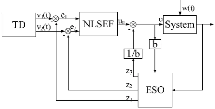
The ADRC originates in the classical PID controller, and retains the core idea of PID error feedback control. The auto disturbance rejection controller is composed of three parts, that’s TD, ESO and NLSEF[5-6]. Their roles are as follows:
c. The function of NLSEF is combining the tracking signal and differential signal generated by TD and the system's estimated state given by ESO with nonlinear function to achieve a control volume. The output of NLSEF is the control volume of the controlled object.
Taking a two-order system for example, its standard ADRC structure is usually as Fig.1[6].
Fig. 1. The ADRC structure of a two-order system
B. The Algorithm of ADRC
There are many nonlinear function forms for the ADRC algorithm, while the classical second order functions of the ADRC algorithm are as follows,
b
z
u
u
or
b
z
u
u
h
r
e
c
e
fhan
u
z
v
e
z
v
e
fe
h
z
z
u
b
fe
z
h
z
z
e
z
h
z
z
h
e
fal
fe
h
e
fal
fe
y
z
e
hfh
v
v
v
h
v
v
h
r
v
v
v
fhan
fh
0
3
0
0
3
0
1
2
1
0
2
2
2
1
1
1
1
03
3
3
0
02
3
2
2
01
2
1
1
1
1
2
2
2
1
1
0
2
1
/
,
,
/
)
(
)
,
,
,
(
,
)
(
)
(
)
(
)
,
25
.
0
,
(
),
,
5
.
0
,
(
,
)
,
,
,
(
(1)Where, fal( x, α, d) is a nonlinear function, written as
d
x
x
sign
x
d
x
d
x
d
x
fal
|
|
),
(
|
|
|
|,
/
)
,
,
(
1
(2)
)
(
))
(
/
(
2
/
))
(
)
(
(
)
(
2
/
))
(
)
(
(
2
/
)
)(
(
|)
|
8
(
2
2
0
1
0
2
1
0
1
2
0
2
a
rsign
s
a
sign
d
a
r
fhan
d
a
sign
d
a
sign
s
a
s
a
y
a
a
d
y
sign
d
y
sign
s
d
a
y
sign
a
a
y
d
d
a
a
x
y
x
h
a
h
r
d
a
a
y
y
(3)In the formula (1), v1 is the tracking signal of the given input signal, while v2is the differential signal. u is
the control volume and the input signal of controlled object, while y is the output signal. Both u and y are the input signals of ESO. The output signals are z1, z2 and z3. z1and z2are the variables of the estimated state. z3is the
estimated signal on which the internal disturbance and external interference are working, that is the estimated signal of total disturbances. r0,β01,β02,β03,c,r,h,h1 and b0are parameters of ADRC. h is the simulation step.
r0is determined according to the speed of the transition process and the system's ability to withstand disturbance.
It just influences the tracking accuracy and the transition process time but has no influence on the output. Once regulated, it can be fixed. β01,β02 and β03 can be determined by system's sampling step. Therefore, only four
parameters need to regulate. They are control gain r, damping coefficient c, precision factor h1and compensation
factor b0.
III. Simulink Modeling of ADRC
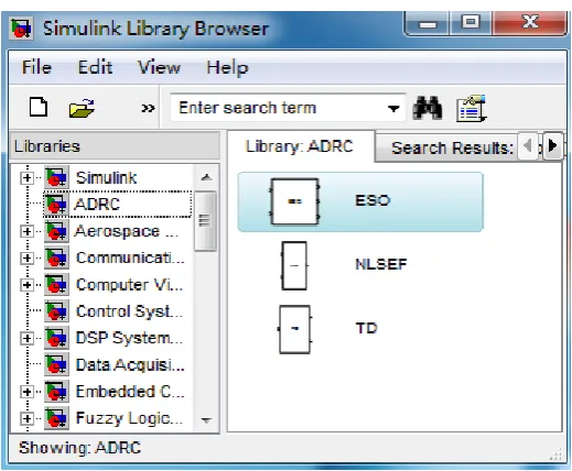
Under Simulink environment, the simulation model is built according to the ADRC algorithm.The ‘Edit Mask’ command in Simulink provides all the operations and value settings of edited module while packaging subsystem. It can mask any subsystem.After packaging, the subsystem can be used to replace the parameter box and content with a simple one. The encapsulated subsystem can be put into a new defined library. Through that, a user-defined library[7-8] can be created and displayed in the library browser.
A. Subsystem Encapsulation Process
Encapsulation is masking the subsystem into a module that has special function. The module as the inherent module in Simulink has its own icon and parameter dialog box. Double click the module a dialog box in which one can set parameter values[9] will be popped up. Take the ESO of typical second order ADRC system as an example, it gives a detail introduction of the subsystem masking process. The algorithm of the ESO is characterized as follows,
)
(
)
(
)
,
25
.
0
,
(
)
,
5
.
0
,
(
0
02
3
2
2
01
2
1
1
1
1
u
b
fe
z
h
z
z
e
z
h
z
z
h
e
fal
fe
h
e
fal
fe
y
z
e
According to the ESO algorithm, with the basic module of Simulink, the simulation model of ESO is established and shown in Fig. 2 (a). In the process of modeling, the nonlinear function fal( x, α, d) of the algorithm should be written into the M-file. Then the M-file is called by the MATLAB FUNCTION[10-12]module to complete the establishment of the model. When packaged, the subsystem is able to be named, described and illustrated. Meanwhile, the input data window can be designed. The ESO subsystem masking steps are as follows.
a. Create an encapsulation dialog prompt
Create a subsystem encapsulation: Select a subsystem module and Edit Mask command from the Edit menu. Add the five parameters h, belta01, belta02, belta03 and b0 of the ESO into the parameter option page. Each
parameter is defined as an edit control. Then users can set values in the dialog box.
b. Create module descriptions and help texts
Mask types, mask descriptions and mask help texts can be defined in the documentation option page. Through them you can edit the module mask types, descriptions and help texts.
c. Create module icon
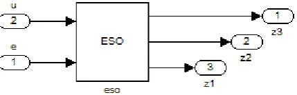
Through the above two steps, a defined dialog box is created for the ESO subsystem. But the subsystem module is still shown as a usual Simulink subsystem icon which is not easy to identify. Simulink provides a group of drawing commands with which can display text, show transfer function, draw a curve or more curves as the subsystem icon. Users can draw self-defined module icon with the MATLAB language written into the "Drawing Commands" edit box in icon option page. For example, if the "disp('ESO')" command is written, "ESO" will be shown as a subsystem mask icon. With all the above finished, the subsystem encapsulation is completed. The packaging subsystem is shown in Fig. 2 (b), where u is an input signal, e is an error signal. z1and
z2are the variables of an estimated state.z3 is the real-time estimate signal of the internal disturbance and external
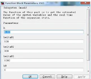
interference. If a subsystem module is double clicked, a parameter setting window will be shown in Fig. 2 (c), and users can change parameter values directly. TD and NLSEF can also be established in the same way. The model of the second order ADRC is shown in Fig. 3.
Fig. 2(a). The simulation model of an ESO subsystem
Fig. 2(c). The parameter setting window
Fig. 3. The model of ADRC
B. User-defined Library
Fig. 3. The defined ADRC library
IV. Simulations
Through the above method, model and simulate the given object. And its form is as follows.
x
y
bu
t
t
w
x
x
f
x
x
x
1
2
1
,
,
(
),
)
(
'
'
2 2 1
(5)
Where, w(t) is external disturbance variable, u is control variable, b is magnification factor, y is output variable, f (x1, x2, w(t), t) is the total external and internal disturbances function.
Set function f (x1, x2, w(t), t) as:
Setsystem parameters as: b=1,γ1 =γ2=1,ω1 =0.6,ω2 =0.7,ω= 1. Set control object:v0=-sign(t-10), namely
the first 10 seconds the value is 1.0, after 10 seconds the value is -1.0, it's called jump function. According to experience and experiments, set controller parameters as: h=0.01, r0 =2, β01=100, β02=300, β03=1000, r=5,
c=0.3, h1=0.03.
According to the above modeling method and operation steps in section III, an ADRC for the above object is designed and modeled. The model is shown in Fig. 4. The simulation results are displayed in different scopes, as shown in Figs. 5, 6 and 7.
Fig. 4. The simulation model of an ADRC system
)).
(sin(
5
.
0
)
(
),
(
)
cos(
)
cos(
)
,
,
(
1
2
1
1
1
2
2
2
wt
sign
t
w
t
w
x
t
w
x
t
w
t
x
x
f
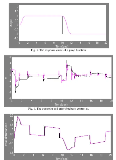
Fig. 5. The response curve of a jump function
Fig. 6. The control u and error feedback control u0
Fig. 7. The total disturbance and its estimation curve
Fig. 5 is the response curve of the system and shows that the system response rapidly and has no overshoot. Fig. 6 shows the curves of the whole control u(t) and error feedback control u0(t). Fig. 7 shows the curves of
system's total disturbances and its estimated values. Through fig7, it's obvious that ESO can estimate and compensate well about the real time action f(x1,x2,t,w(t)) of system's total disturbances. Through the system's
disturbance compensation, it can compensate the original system to be a linear integral tandem system. Then with the error feedback method, the closed-loop has a satisfactory performance and the auto disturbance function of ADRC has been realized.
modeling is practical and valid.
REFERENCES
[1] Han Jing-qing. Active Disturbance Rejection Control Technique-the technique for estimating and compensating the uncertainties(M).Beijing: National Defense Industry Press, 2008
[2] Ja Ya-fei. Active Disturbace Rejection Controller's Research and Its Application[D]. YanShan University, 2013
[3] Ma You-jian, Liu Zheng-gao, Zhou Xue-song, Wang Xin-zhi. Analysis on Principle of ADRC[J]. Journal of Tianjin University of Technology,2008,24(4)
[4] Zhou Jian-xin, Fu Chuan-xiu, Liu Ai-ping. Simulink Simulation and Encapsulation of Second Order Circuit[J]. Journal of Jiamusi University: Natural Science Edition,2007,25(6):733-734.
[5] Meng Fan-dong. Study of Design and Application for the ADRC[D]. Harbin University of Science and Technology,2009 [6] Lei Zheng-ling, Guo Chen, Liu Yang. ADRC Controller Used in Dynamic Positioning System of a Rescue Ship[C]. Proceedings
of the 10th World Congress on Intelligent Control and Automation, 2012.7
[7] Li Ying, Zhu Bo-li, Zhang Wei. SIMULINK Dynamic System Modeling and Simulation[M]. Xi'an: Xi'an Electronic and Science University Press,2004:224-228.
[8] Hu Lin-jing, Sun Zheng-shun. Build and Encapsulate Custom Block in SIMULINK[J]. Journal of System Simulation,2004,16(3) [9] Zhang De-feng. MATLAB/SIMULINK Modeling and Simulation Examples[M]. Beijing: Machinery Industry Press,2010.1 [10] Huang Zhong-lin. MATLAB Implementation of Automatic Control Theory[M]. Beijing: National Defense Industry Press, 2007.2 [11] Fan Jing, Liu Shu-jun, Gai Xiao-hua, Cui Shi-lin. Application and Examples of MATLAB Control System[M]. Beijing: Tsinghua
University press,2008.5