Fast Graph Transformation based Direct Solver Algorithm for Regular Three Dimensional Grids

Fast graph transformation based direct solver

algorithm for regular three dimensional grids

Marcin Sieniek

1*

1 _{AGH University of Science and Technology, Krakow, Poland}

[email protected]

Abstract

This paper presents a graph-transformation-based multi-frontal direct solver with an optimization technique that allows for a significant decrease of time co mplexity in some multi-scale simulations of the Step and Flash Imprint Lithography (SFIL). The mu lti-scale simulation consists of a macro-scale linear elasticity model with thermal expansion coefficient and a nano-scale mo lecular statics model. The algorith m is exemp lified with a photopolimerization simulation that involves densification of a polymer inside a feature followed by shrinkage of the feature after removal of the temp late. The solver is optimized thanks to a mechanis m of reusing sub-domains with similar geometries and similar material properties. The graph transformation fo rmalis m is used to describe the algorith m - such an approach helps automatically localize sub-domains that can be reused.

Keywords: step-and-flash imprint lithography, multi-scale, graph transformations, multi-frontal solver

1

Introduction

The paper presents a multi-scale, graph-transformation-system-powered approach to modeling of the Step-and-Flash Imp rint Lithography (SFIL). SFIL is a modern pattering process that uses photopolymerization in order to replicate a template onto a substrate (Co lburn et al. 2001) andprocess can be simulated in macro -scale as linear elasticity with thermal expansion coefficient (Hughes 2000). In some areas of the computation domain though, the molecular statics model is employed to complement fin ite elements and thus - improve the solution (Paszynski et al. 2005). Since three dimensional finite element method simulations are co mputationally expensive (Demkowicz at al. 2007), a multi-frontal solver algorith m is used in this study. A reuse technique is proposed to benefit from some of the regularities that problems from this domain present.

Multi-frontal solvers are considered some of the most advanced direct solvers suited for solving linear systems of equations (Geng et al. 2006, Duff and Reid 1983, Duff and Reid 1984). Graph transformation systems have been previously used to model mesh generation and for mu lti-frontal

* _{corresponding author}

Volume 29, 2014, Pages 1027–1038

ICCS 2014. 14th International Conference on Computational Science

solvers for examp le in (Paszynska et al. 2008, Paszynska et al. 2012b, Paszynski et. al 2009a, Paszynski et al. 2009b, Paszynska et al. 2012a). However in this work, a new graph transformation system, allowing for efficient reuse of identical sub-branches of the elimination tree is introduced.

The graph transformation system presented in this paper for reuse of identical sub-trees has been also utilized for modeling mesh generation and adaptation with CP-graphs (Paszynska et al. 2012a, Paszynska et al. 2012b, Paszynska et al. 2009, Strug et al. 2013) and hyper-graphs (Slusarczyk et al. 2013). Th is graph model can be also used for expressing the classical multi-frontal solver algorithm (Paszynski and Schaefer 2010, Paszynski et al. 2010).

Finally, it is also possible to obtain the linear co mputational cost direct solver using some other topological features of the refined meshes (Szymczak et al. 2013, Paszynski et al. 2013).

2

Step-and-Flash Imprint Lithography

Step and flash imp rint lithography (SFIL) is a patterning process utilizing photopolymerization to replicate the topography of a template onto a substrate (Bailey et al. 2002, Co lburn et al. 2001, Bu rns et al. 2004).

The SFIL process can be described in the following six steps, as it is illustrated in Figure 1. 1) dispense. The SFIL process employs a template / substrate alignment scheme to bring a rigid

template and substrate into parallelis m, trapping the etch barrier in the relief structure of the template,

2) imprint. The gap is closed until the force that ensures a thin base layer is reached, 3) exposure. The template is then illuminated through the backside to cure etch barrier,

4) separate. The template is withdrawn, leaving low-aspect ratio, high resolution features in the etch barrier,

5) breakthrough etch. The residual etch barrier (base layer) is etched away with a short halogen plasma etch,

6) transfer etch. The pattern is transferred into the transfer layer with an anisotropic o xygen reactive ion etch, creating high-aspect ratio, high resolution features in the organic transfer layer.

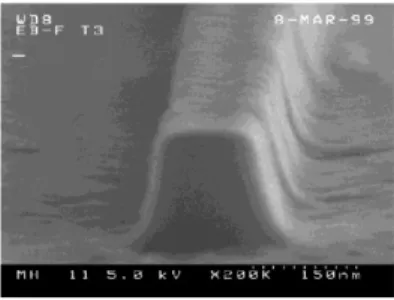
Figure 1: Step and Flash Imprint Lithography Figure 2: Shrinkage of the feature after removal of the template

Photopolymerization is often acco mpanied by densification. The interaction potential between photopolymer precursors undergoing free radical poly merization changes from van der Waals’ to

covalent. The average distance between molecules decreases and causes volumetric contraction. Densification of the SFIL photopolymer (the etch barrier) may affect both the cross sectional shape of the feature and the placement of relief patterns. The exemp lary shrin kage of the feature measured after removing the template is presented in Figure 2.

2.1

Macro scale model

The linear elasticity model with thermal expansion coeff icient is used to verify the material response of poly merized networks in cu red etch-barrier layers that are formed during the third step of the SFIL process.

Strong formulation. Given g_i:*_Di xog_i x 0R, , D_kl and Vij0, find ui::oR the

displacement vector field such that 0 ,j ij

V

in : (1) i i g u in i D * (2)

where V_ij is the stress tensor, defined in terms of the generalized Hooke’s law

0 ij kl kl ijkl ij c H TD V V (3) ijkl

c elastic coefficients (known for a g iven material), Vij0 initial stress. Hij0 initial strain,

temperature,

kl

D thermal expansion coefficients,

H

_ij is the strain tensor, defined to be u_i,j , the symmetric part of the displacement gradients

2 , , ,j i j ji i ij u u u

H

(4)

where u_i displacement vector, u_i,j displacement gradients.

Weak formulation. The weak formu lation is obtained by multip lying (1) by test functions w_iV_i

and integrating by parts over :.

0 , : :

_³

_³

* : d n w d w_{i j}V_{ij i}V_{ij j} (5)

Since V_ij is symmetric tensor, then w_i,j

V

_ij w_i,j

V

_ij (compare Hughes 2000), and wi 0 on *, we get 0 , :

³

: d wijVij (6)

Finally, we substitute (3) into (6) and get

: : : _{³ ³} ³ : : : d w d c w d u c w_{(i,j) ijkl k,l} T _{(i,j) ijkl}D_{kl i,j}V_ij0 (7) since

H

_ij u_i,j .

Abstract index-free notation. For imp lementation issues, the most convenient is the following form:

Find uV such that

w,u

Α

w Σw a for all wV (8) Where

_³

: : d u Dε w ε u w, a T (9) :

³

: d Dα w ε w Α T T (10) :

³

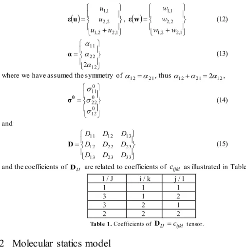
: d 0 T_σ w ε w Σ (11) Here T T

° ¿ ° ¾ ½ ° ¯ ° ® ­ _2,1 2 , 1 2 , 2 1 , 1 u u u u u ε , ° ¿ ° ¾ ½ ° ¯ ° ® ­ _2,1 2 , 1 2 , 2 1 , 1 w w w w w ε (12) ° ¿ ° ¾ ½ ° ¯ ° ® ­ 12 22 11 2D D D α (13)

where we have assumed the symmetry of D₁₂ D₂₁, thus D₁₂D₂₁ 2D₁₂,

° ¿ ° ¾ ½ ° ¯ ° ® ­ 0 12 0 22 0 11

V

V

V

0 σ (14) and ° ¿ ° ¾ ½ ° ¯ ° ® ­ 33 23 13 23 22 12 13 12 11 D D D D D D D D D D (15)

and the coefficients of D_IJ are related to coefficients of cijkl as illustrated in Table 1.

I / J i / k j / l

1 1 1

3 1 2

3 2 1

2 2 2

Table 1. Coefficients of DIJ cijkl tensor.

2.2

Molecular statics model

Let us consider a regular rectangular 3D grid with interacting particles , as presented in Figure 3a.

(a) (b)

Figure 3: (a) 3D domain with interacting particles. (b) pair of interacting particles in the initial and equilibrium configurations

Each particle interacts with its 26 neighbours. For each pair of interacting particles D and E, we can distinguish their in itial configurations p_D, p_E and (unknown) equilibriu m configurations xD, xE,

compare Figure 3b.

The following molecular statics models are considered:

x Linear model assuming small deformations and quadratic potentials. In this model the force between pair of interacting particles D and E is given by

α β α β αβ p p p p F ' _{r r} o r k_{DE DE DE DE} (16)

where k_DE is the spring stiffness coefficient, r_DE'r_DE x_βx_α is the length of the spring in the

equilibriu m configuration, x_α,x_β represents the (unknown) equilibriu m configuration of particles,

r

_DE0

is the length of the un-stretched spring, p_α,p_β represents the initial configuration o f particles. The

small deformations are observed here, which imp lies the direction of the interparticle forces along the initial spring aligments p_βp_α.

x Non-linear model allowing for large deformations, with quadratic potentials. In this model the force between pair of interacting particles D and _E is given by

α β α β αβ x x x x F ' _{r r} o r k_{DE DE DE DE} (17)

The large deformations are observed here, which imp lies the direction of the interparticle forces along the resulting spring alignments x_βx_α.

x Non-linear model allowing for large deformations, with Lennard-Jones potentials. In this model the force between pair of interacting particles D and _E is given by

α β α β α β α β αβ x x x x x x x x F » » » ¼ º « « « ¬ ª ¸ ¸ ¹ · ¨ ¨ © § ¸ ¸ ¹ · ¨ ¨ © § 1 DE 1 DE DE DE DE DE DE DE V V V n m n m C ₍₁₈₎

which results from Lennard-Jones potential

¸¸ ¸ ¹ · ¨¨ ¨ © § ¸ ¸ ¹ · ¨ ¨ © § ¸ ¸ ¹ · ¨ ¨ © § DE DE DE DE DE DE DE DE DE V V n m r r C r V (19)

where

V

_DE,

n

_DE and

m

_DE are Lennard-Jones potential parameters.

The mo lecular statics problem consists in finding the equilib riu m configuration of particles satisfying

¦

EFαβ 0

(20)

for D=1,...,N (total nu mber of particles). More mathematical details of the molecular statics model formulation are presented in (Paszynski et al. 2005).

2.3

Coupling between the macro-scale and nano-scale models

The macro-scale and nano-scale models are coupled by identifying the particles located on the interface of the nano-scale domain with the corresponding nodes of the FEM mesh, located on the interface of the macro-scale mesh.

In such the case, we solve the mo lecular statics equations inside the nano-scale domain, and the linear elasticity with thermal expansion coefficient discretized by FEM inside the macro-scale do main, while the interface between macro- and nano-scales is treated in the special way. The nodes of the FEM mesh, fro m the point of v iew of the nano-scale model are identified with particles represented by their positions x_α, while fro m the point of view of the macro-scale model, the nodes are understood in the classical way like degrees of freedo m, representing the displacements u_α. It implies the additional coupling equations α α α α p x p u ' ₍₂₁₎

for each particle (FEM mesh node) D located on the interface between nano- and macro-scales. In practice, it is not necessary to add the coupling equations (21) to the system, but only to aggregate the FEM and MS equations to the same global matrix.

3

Numerical solver with a graph transformation system

description

In this section a mu lti-frontal solver is described. In order to present the algorith m performed by the solver, graph transformation systems are used. Such a formalis m allows for describing steps of an algorith m as a set of transformations that alter a graph representing a computational mesh and attribute it with computational data. As a result it's easier to determine the algorith m's properties, time complexity and determine whether a given algorithm is legal.

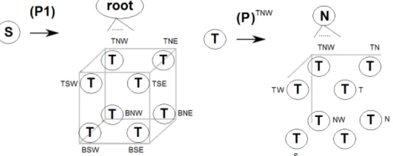
The first step of the solver algorith m is to generate the computational mesh. It is done by executing a sequence of graph transformations that generate a graph structure representing computational mesh. The first graph transformation is presented on left panel in Figure 2. The productions replace the starting graph containing only a single vertex S with a graph representing a single hexahedral element with eight nodes. The following graph transformations replace some nodes by sub-graphs that represent smaller elements. Graph nodes as well as graph transformations are attributed by the location over a rectangular domain. The transformation (P)TNWfro m right panel in Figure 2 is replicated for different locations, fo r {TNW,TNE,TSW,TS E,BNW,BNE,BSW,BS E} where T and B stands for top and bottom, and N, S, W, E stand for north, south, west, east.

Figure 4: Exemplary graph transformations for generating of the structure of the mesh

The exemp lary derivation of an eight-element mesh is presented in Figure 4. In the first step, production (P1) is executed, in the second step, productions (P)TNW - (P)TNE - (P)TSW - (P)TSE - (P)B NW - (P)B NE - (P)B SW - (P)BSEareexecuted to obtain the eight fin ite element mesh. The graph representing the mesh has hierarchical tree -like structure storing the history of graph transformations derivation. To obtain larger meshes, it is necessary to add graph transformations for locations like

{T,B,N,S,W,E,TN,TS,TW,TE,BN,BS,BW,BE,NE,NW,S E,SW}, co mpare labels of the left bottom sub-graph at Figure 5.

Figure 5: Derivation of eight finite element mesh

Figure 6: Graph transformations for identification of macro- and nano-scale elements

The next step of the solver algorith m consists in identification of macro -scale and nano-scale elements. Notice that graph nodes labeled with N actually represent particles (over nano-scale elements) or finite element method nodes (over macro-scale elements). Thus, the elements are represented by patches of eight nodes. In the exemp lary mesh presented in Figure 5 there are eight elements denoted by different colors.

This identification is performed by graph transformation presented in Figure 6. The macro-scale elements are attributed by Young modulus and Poisson ratio values. The nano -scale elements are attributed by parameters of the spring force parameters k_DE.

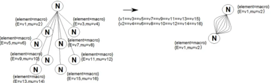
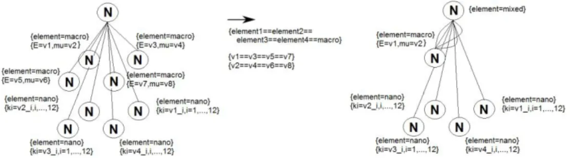
Figure 8: Exemplary graph transformation for partial identification of macro-scale with identical material data

The resulting tree structure can be directly utilized by the mu lti-frontal solver algorith m (Paszynski et al. 2010, Paszynski and Schaefer 2010). Ho wever, in th is work a more sophisticated approach, featuring a re-use optimization technique, is proposed. It is based on an observation, that if we postpone the resolution of the domain boundary to the top of the elimination tree, given a regular mesh with equal coefficients, the LU factorized local matrices for different finite elements are the same and hence can be reused.

Thus, the third step of the solver algorith m consists in an identification of identical sub-branches of the elimination tree, fo r the reuse of partially LU factorized matrices. An exemplary graph transformation for such an identification is presented in Figure 7. Such a graph transformation checks if all eight son elements are macro-scale elements and whether the corresponding Young modulus and Poisson ratios are identical. If this is the case, the eight son element nodes are reduced to one representative node, so the LU factorization can be perfo rmed only once and father node can merge eight identical matrices from the same representative son node.

Another, more co mp licated case for the identification is presented in Figure 8. In this example only four son elements are macro-scale with identical Young modulus and Poisson ratio values. The four identical macro -scale elements are reduced to one representative element, however the nano-scale elements are stochastic in their nature and cannot be reduced.

Finally, on a modified elimination tree, the multi-frontal solver algorithm can be executed:

1 function frontal_elimination(node)

2 if new_schur_matrix already computed for the node then 3 return schur_matrix

4 if node is a leaf then

5 generate local system assigned to node

6 excluding boundary conditions

7 else

8 loop through son_nodes

9 schur_matrix = frontal_elimination(son_node)

10 merge schur_matrix into new_system

11 end loop 12 end if

13 find fully assembled nodes and eliminate them

14 return new_schur_matrix

15 end function

Notice that in case of representative nodes in line 9, the same node of the elimination tree is actually called many times and line 2 p revents from re-co mputing the identical Schur co mp lement matrices many times. The fo rward elimination algorithm is fo llo wed by analogous backward substitution.

4

Numerical results

In this section numerical results presenting the shrinkage of the feature after removal of the template. It is assumed that the polymer network has been damaged during the removal of the template, and thus the inter-particle forces are weaker in one part of the mesh.

The problem has been solved first by using pure nano-scale approach, with non-linear model allo wing for large deformations, with quadratic potentials (17). The resulting equilibriu m configurations of polymer network particles are presented in Figure 9 and 10. The damage has been modeled here by assuming smaller values of the spring stiffness coefficients k_DE.

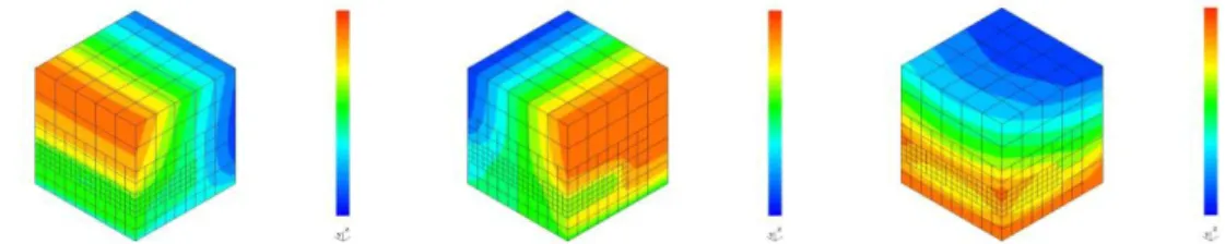
Then, the problem has been solved again by using the multi-scale approach. The part of the mesh with undamaged poly mer has been modeled by the macro -scale approach, with Finite Element Method. The part o f the mesh with the damaged polymer, denoted in Figure 11 by red co lor, has been modeled by the nano-scale approach with linear model assuming small deformations and quadratic potentials. The results – the x, y and z co mponents of the vector displacement field are presented in Figures 8, 9 and 10. The damage of the poly mer, modeled by weakening the inter-particle forces results in slight lean of the feature, illustrated in Figure 5 fo r the nano-scale model, and in Figure 8, for the macro-scale model. The displacement fields are similar in both nano-scale and macro-scale simulations.

Figure 9: X, Y and Z components of the displacement vector field for the interior modeled by linear elastictity with thermal expansion coefficient

Figure 10: Results of the non-linear model allowing

for large deformations, with quadratic potentials Figure 11:blue color denotes the macro-scale domain with FEM 3D mesh for multi-scale simulations. The model, the red color denotes the nano-scale domain with MS model

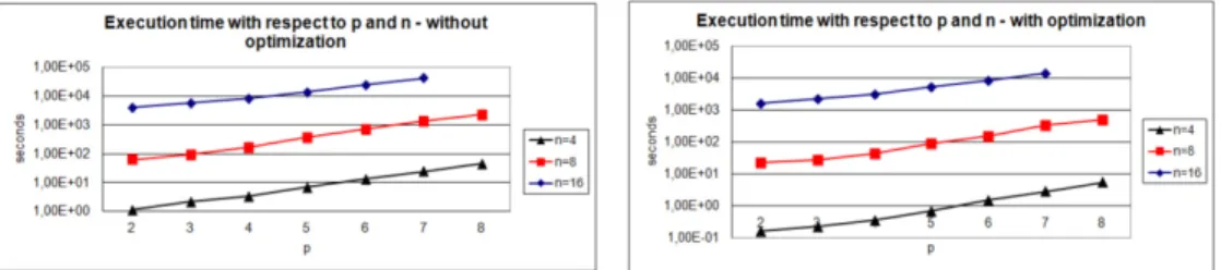
To conclude this section, let us look at the co mparison of the execution times of the graph transformation based multi-frontal solver executed with and without the reuse technique. The computations have been performed sequentially on a cluster node with Dual-Core AMD Opteron processor clocked at 2.6 GHz with 32 GB using a Fortran 90 implementation.

The results are presented in Figures 12-13. The horizontal axis denotes different polynomial orders of appro ximations utilized over the macro-scale do main (p parameter). Different lines correspond to different number o f elements in each direction (n parameter). The resulting speedup of the reuse solver algorithm is presented in Figure 13.

Figure 12: Left panel: Execution time of the solver without reuse Right panel: Execution time of the solver with reuse

Figure 13: Speedup of the reuse solver

5

Conclusions & future work

In this paper a fast multi-frontal solver algorithm with a reuse technique has been presented along with a theoretical description using graph transformation systems. The benefits from this technique have been exemp lified on a problem fro m nano-lithography domain, however the technique can be used on a wider class of problems defined on a regular domain with equal material coefficients and should offer significant savings especially in setups where parallel processing is not an option.

The technique is limited to sequential execution though. The single-point coupling method used is also known to have limitations (Bau man et al. 2008) so the future work could include imp lementing the Arlequin interface instead. Apart fro m that, it would be desirable to define the boundaries of applicability of the re-use technique formally and define the conditions of a problem that help maximize the outcome.

6

Acknowledgement

The work has been supported by the AGH University of Science and Technology dean grant.

References

Bailey, T. C., Colburn, M. E., Choi, B. J., Grot., A., Ekerdt, J. G., Sreenivasan, S. V., Willson C. G. (2002) Step and Flash Imprint Lithography: A Low-Pressure, Room Temperature Nanoimprint Patterning Process. Alternative Lithography. Unleashing the Potentials of Nanotechnology. C. Sotomayor Torres (editor) Elsevier

Bau man, P.T., Ben Dhia, H., Elkhodja, N., Oden, J.T., Prudhomme, S. (2008). On the application of the Arlequin method to the coupling of particle and continuum models, Computational Mechanics, vol. 42, pp. 511-530

Burns, R. L., Johnson, S. C., Sch mid, G. M., Kim, E. K., Dickey, D. M. D., Meiring, J., Burns, S. D., Stacey, N. A., Willson C. G. (2004). Mesoscale modeling for SFIL simu lating poly merization kinetics and densification, Proceedings of SPIE

Colbu m, M. E., Suez, I., Choi, B. J., Meissi, I., Bailey, T., Sreenivasan, S. V., Ekerdt, J. E., Willson, C. G. (2001). Characterization and modeling of volumetric and mechanical properties for SFIL photopolymers. Journal of Vacuum Science and TechnologyB, vol. 19, pp. 6-20.

Demkowicz L., Ku rtz J., Pardo D., Paszynski M., Zdunek A. (2007). Co mputing with hp-Adaptive Finite Element Method. Vol. II. Frontiers: Three Dimensional Elliptic and Maxwell Problems. Chapmann & Hall / CRC Applied Mathematics and Nonlinear Science

Demkowicz, L., Kurtz, J., Pardo, D., Paszyński, M., Rachowicz, W., Zdunek A. (2008). Computing with hp Adaptive Finite Elements. Volume 2. Frontiers: Three Dimensional Elliptic and Maxwell Problems with Applications

Duff I. S., Reid J. K. (1984). The mu ltifrontal solution of unsymmetric sets of linear systems, SIAM Journal of Scientific and Statistical Computing, vol. 5, pp.633-641.

Duff I. S., Reid J. K. (1983). The mu ltifrontal solution of indefinite sparse symmetric linear equations,

ACM Transations on Mathematical Software, vol. 9, pp. 302-325

Geng P., Oden T. J., van de Geijn R. A. (2006) . A Parallel Multifrontal Algorith m and Its Implementation, Computer Methods in Applied Mechanics and Engineering, vol. 149, pp.289-301.

Hughes T. J. R. (2000). The Finite Element Method. Linear Statics and Dynamics Finite Element Method Analysis, Dover

Paszynska, A., Grabska, E. and Paszynski, M. (2012a). A graph grammar model of the hp adaptive three dimensional finite element method. part I, Fundamenta Informaticae, vol. 114 (2), pp. 149-182.

Paszynska, A., Grabska, E. and Paszynski, M. (2012b). A graph grammar model of the hp adaptive three dimensional finite element method. part II, Fundamenta Informaticae vol. 114 (2), 183-201. Paszynska, A., Paszynski, M., Grabska, E. (2008). Graph transformations for modeling hp-adaptive fin ite element method with triangular elements, Lecture Notes in Computer Science, vol. 5103 pp. 604–613.

Paszynska, A., Paszynski, M., Grabska, E. (2009). Graph Transformations for Modeling hp-Adaptive Fin ite Element Method with Mixed Triangular and Rectangular Elements , Lecture Notes in Computer Science, vol. 5545, pp.875-884

Paszynski, M. (2009a). On the parallelization o f self adaptive hp-finite element methods part I. composite programmable graph grammar model, Fundamenta Informaticae, vol. 93 no. 4, pp. 411–434.

Paszynski, M. (2009b). On the parallelization of self-adaptive hp-fin ite element methods part ii. partitioning co mmunication agglo meration mapping (PCAM) analysis, Fundamenta Informaticae,

vol. 93 no. 4, pp. 435–457.

Paszynski, M., Barabasz, B., Schaefer R. (2007). Efficient Adaptive Strategy for Solving Inverse Problems, Y. Shi et al. (Eds.): ICCS 2007, Part I, Lecture Notes In Computer Science 4487, pp.342–349

Paszynski, M., Pardo, D., Paszynska, A. (2010). Parallel mu lti-frontal solver for p adaptive fin ite element modeling of mu lti-physics computational problems, Journal of Computational Science, vol. 1, no. 1, pp. 48-54.

Paszynski, M., Pardo, D., Calo, V. M. (2013). A direct solver with reutilization of LU factorizations for h-adaptive finite element grids with point singularities , Computers & Mathematics with Applications, vol. 65 (8), pp.1140-1151

Paszynski, M., Ro mkes, A., Collister, E., Meiring, J., Demkowicz, L.F., W illson, C. G. (2005). On the modeling of Step-and-Flash Imprint Lithography using molecular statics models. ICES Report, vol. 05-38

Paszynski, M., Schaefer R., (2010). Graph grammar driven partial differential eqautions solver,

Concurrency and Computations: Practise and Experience, vol. 22, no. 9, pp.1063-1097.

Strug, B., Paszynska, A., Paszynski, M . (2013). Using a graph grammar system in the finite element method, International Journal of Applied Mathematics and Computer Science, vol. 23(4), pp.839-853

Slusarczy k, G., Paszynska, A. (2013). Hypergraph Grammars in hp-adaptive Finite Element Method,

Procedia Computer Science, vol. 18 pp.1545-1554

Szy mczak, A., Paszynska, A., Gurgul, P. (2013). Graph Grammar Based Direct Solver for hp-adaptive Fin ite Element Method with Po int Singularities , Procedia Computer Science, vol. 18, pp. 1594-1603