A Feature-Based Call Graph Distance Measure for Program Similarity Analysis

(1)

A Feature-Based Call Graph Distance Measure for

Pro-gram Similarity Analysis

Simo Linkola

Master’s Thesis

UNIVERSITY OF HELSINKI

Department of Computer Science

(2)

Faculty of Science Department of Computer Science

Simo Linkola

A Feature-Based Call Graph Distance Measure for Program Similarity Analysis

Computer Science

Master’s Thesis May 13, 2016 54

executable analysis, call graph, feature generation, distance measure

A measurement for how similar (or distant) two computer programs are has a wide range of possible applications. For example, they can be applied to malware analysis or analysis of university students’ programming exercises. However, as programs may be arbitrarily structured, capturing the similarity of two non-trivial programs is a complex task. By extracting call graphs (graphs of caller-callee relationships of the program’s functions, where nodes denote functions and directed edges denote function calls) from the programs, the similarity measurement can be changed into a graph problem.

Previously, static call graph distance measures have been largely based on graph matching techniques, e.g. graph edit distance or maximum common subgraph, which are known to be costly. We propose a call graph distance measure based on features that preserve some structural information from the call graph without explicitly matching user defined functions together. We define basic properties of the features, several ways to compute the feature values, and give a basic algorithm for generating the features.

We evaluate our features using two small datasets: a dataset of malware variants, and a dataset of university students’ programming exercises, focusing especially on the former. For our evaluation we use experiments in information retrieval and clustering. We compare our results for both datasets to a baseline, and additionally for the malware dataset to the results obtained with a graph edit distance approximation.

In our preliminary results we show that even though the feature generation approach is simpler than the graph edit distance approximation, the generated features can perform on a similar level as the graph edit distance approximation. However, experiments on larger datasets are still required to verify the results.

ACM Computing Classification System (CCS):

• _{Information systems~Similarity measure}

• _{Information systems~Clustering and classification}

• Security and privacy~Intrusion/anomaly detection and malware mitigation • _{Theory of computation~Program analysis}

• _{Software and its engineering~Software evolution}

Tiedekunta — Fakultet — Faculty Laitos — Institution — Department

Tekijä — Författare — Author

Työn nimi — Arbetets titel — Title

Oppiaine — Läroämne — Subject

Työn laji — Arbetets art — Level Aika — Datum — Month and year Sivumäärä — Sidoantal — Number of pages

Tiivistelmä — Referat — Abstract

Avainsanat — Nyckelord — Keywords

Säilytyspaikka — Förvaringsställe — Where deposited

(3)

1 Introduction

Trying to determine the function of a piece of software from its executable by other means than running the program is a hard task. Even deciding whether the program will come to a stop, or halt, is undecidable. Analysing the behavior of programs is still needed in, for example, malware1detection.

The history of large scale malware is approximately 30 years old; although, the Cambrian explosion of malware triggered only after the use of internet spread. The term, computer virus, was introduced by Frederick Cohen in 1984 (see [7]), and the first MS-DOS virus, Brain, was detected in 1986. However, the definition of the computer viruses is not entirely agreed upon; hence, the identity of the first program to carry the name has been exposed to debate in the history of computer security [10].

The first viruses until the mid-80’s were largely self-replicating exploits, which did no further harm – excluding the consumption of disc space – to the compromised systems. Afterwards, the evolution of the viruses and other malware has taken a path from damaging boot sector viruses, such as Michelangelo, through e-mail worms and Trojan horses, that bloomed in the late 90’s and early 00’s, to high profile software – e.g., botnets – that are nearly entirely spread for commercial purposes. In the few recent years, malware tailored to the spesific purposes by the military or national agencies has been exposed.

Malware evolution can be generally seen as a two-step race where both steps are carried simultaneously. In the first step, the malware publishing groups and individuals modify the existing malware, and test them against various cutting edge anti-virus programs until the programs don’t recognize the malware anymore. In the second step, anti-virus software groups and companies collect new malware samples and adjust their software to detect them. As the time goes by, also entirely new malware families are created. The new exploits may target previously unknown zero-day vulnerabilities, or existing holes in the security. Thus, the face of the malware detection is ever changing; for example, mobile malware families were said to increase 58% from 2011 to 2012 [34].

The continuously evolving field makes similarity analysis of different malware instances a key point in recognizing the variations of already known malware families, and in detecting the new and unseen exploits. The enhanced detection helps private parties and companies by providing better anti-virus software, 1_{Malware is a general term for various kinds of hostile or intrusive software such as viruses,}

(5)

and efficient classification and clustering aids the analysts in anti-virus software companies to perform justified decisions of the relations between different malware families and variants.

As malware publishers can use tools, such as Mistfall, Win32/Smile and RPME [35], to automatise code obfuscation, it is important to handle similarity analysis in a way that is as resistant as possible to such methods. Therefore, the first proposed methods that compute similarities or edit distances between operational code (opcode) sequences are too unstable as even substantial changes in the code may not change the actual functionality of the program.

A plenty of different approaches have been proposed for more robust malware detection and classification. They can be coarcely divided into two groups: dynamic (behavioral) and static analysis. Dynamic analysis of a malware binary is performed by running the malware in a so called sandbox environment and data from the run is collected in some form; typically as a feature vector or as snapshots of the system states before and after the run. In static analysis, malware binary is disassembled with a dissambler, e.g. IDA Pro [9]. Disassembling yields a dissection of the binary’s inner structures, such as function caller-callee relationships. The drawback of the dynamic analysis is that the data is only captured from one run and may not represent all of the possible behavioral traits. On the other hand, the static analysis may not be able to interpret all of the code’s inner structure, thus yielding only partial or even false information.

The caller-callee relationships acquired by the static analysis can be used to create a call graph of the malware. A call graph of a binary is a directed graph where vertices represent local and non-local functions and edges represent calls between functions.

The call graphs serve as a useful higher abstraction of the program binaries. They are not so prone to simple opcode switching techniques, although they can be relatively easily distorted, e.g. by refactoring a local function into two different functions, where the two functions combined have exactly the same behavior as the non-refactored function.

In most of the works on malware analysis using call graphs, the similarity measure between malware variants is acquired either by using graph edit distance (GED) estimation, maximum common subgraphs or function matching. However, these techniques are still quite vulnerable to code obfuscation techniques that heavily alter the call graph’s structure without altering the functionality of the software.

(6)

approach in this thesis. To compute a distance between call graphs, we do not try to explicitly match local functions between different programs. Instead, we consider as features the sets ofknon-local functions. The non-local functions must be linked together by a call structure where there exists a local function root, such that each non-local function is at mostdth successor of the root. We generate these feature sets from both call graphs, and the distance between the call graphs is then computed to be the distance between the feature sets.

The used distance measure is not limited to the malware analysis, and is, of course, applicable to programs of various kinds. One such task is to analyse how similar programming exercises are. Measuring the distance between the returned exercises can reveal common higher level structures in the exercise solutions, or in extreme cases may even give a hint of plagiarism[15].

We evaluate our features with two datasets: a malware dataset consisting of 193 variants in 24 different familities, and a student dataset consisting of a total number of 366 exercises returned for five different exercise assignments. In our experiments we use retrieval tasks and clustering to analyse how well the proposed features perform. In addition, the proposed features are compared against results obtained with GED approximation for the malware dataset.

The rest of the thesis is organized as follows. First, previous related work in the field is reviewed. Then, basics of graphs and call graphs are explained. After different graph related properties, the graph features and in particular the proposedd-reachablek-gram features are discussed, and an attempt to analyse and define what makes a good call graph feature is made. After the proposed features are introduced, we give an overall view of the two datasets used in this thesis. Then, the call graph features are used to perform clustering and retrieval tasks on the two datasets and the performance of the features is evaluated. Following the experiments is a discussion about the validity of the results, and the thesis ends with conclusions and notions about the possible future work.

2 Related Work

In this section we will give a short overview of the work previously done in related areas. However, before we can delve deeper, we must make a clear cut between two different forms of malware analysis: malware detection, and malware classification. Even though the malware domain has been studied extensively, these terms are used vaguely or with mixed meanings in the existing literature. The most prominent one is malware detection. In this thesis, the malware detection

(7)

is used to specify the act of detecting when the existing malware variants infiltrate or compromise a system. The detection is typically run by anti-virus software and uses finger printing and/or heuristics to detect possible threats to the system. Of course, some finger prints or heuristics may also match new malware variants, but the methods do not separate these from the existing ones.

On the other hand, malware classification and clustering are done by anti-virus companies analysts in order to retrieve more information of the new and existing variants and families, and to define their relationships. However, as malware detection is based on the work done by the analysts, the two are closely related and the tools and techniques developed for one can often be applied to the other. The history of malware classification is as old as the first damaging malwares. Early work based on treating the malware binary as a sequence of operational

codes(opcode). Malware variants were detected and classified based on various

versions of opcode fingerprinting techniques (opcode sequences with various ways to denote wildcards, etc.) [35].

The search for resilient methods to classify self-morphing and obfuscated malware variants into new and existing strains has lead to diverse field of study which can be roughly divided into two sections: behavioral2_{and static analysis.}

Although, in many occasions static and behavioral techniques are combined into hybrid methods for a more complete approach.

Behavioral analysis runs malware variants in a so called sandbox environment and collects information by monitoring run-time system calls. This information can then be used, e.g. to create a feature vector which is compared against vectors acquired from other variants.

Using call graphs acquired via static analysis to examine similarities in benign or malware binaries is another popular approach. Techniques revolving around call graphs can be generally divided into three closely related, but distinct approaches: finding maximum common subgraphs (MCS), finding graph edit distances (GED) [31], and finding vertex or edge matchings between the call graphs based on local neighborhoods.

Carrera and Erdélyi [6] developed a python package (IDAPython) for easy extraction of call graphs from IDA Pro [9]. Similarity between call graphs is based on function matching where local functions are matched based on their call-tree signature, which is a binary vector expressing called non-local functions, and control flow graph (CFG) signatures; the list of edges connecting basic blocks in function’s CFG. The method is evaluated using several small case studies, and

(8)

constructing a phylogenetic tree from the whole dataset.

Briones and Gomez [4] continue the work done by Carrera and Erdélyi [6], and modify their function matching and similarity metric. For each local function, a signature is computed from the sequence of its opcodes and used for fast local function matching. Furthermore, the CFG signatures are altered to contain number of basic blocks, number of edges and number of subcalls.

Park et al. [25] use behavioral call graphs and define a similarity metric based on maximal common subgraphs (MCS). The similarity between two graphs is derived from the number of nodes in the MCS divided by the number of nodes on the larger call graph. They evaluate their method with 300 malware variants (6 families each consisting of 50 samples) and 80 benign executables, and obtain tentatively promising results.

The first large scale work which utilizes GED approximation to call graphs in malware classification was done by Hu et al. [12] . The GED approximation used is a bipartite graph matching proposed in [26, 27], which is further optimized. Bipartite graph matching uses the Hungarian algorithm originally proposed by Kuhn [20]. Fundamentally, Hu et al. construct the whole system to store and query malware in a two-layered hierarchical database to efficiently index the malware and therefore accelerate the queries to database. Both of the layers are trees, where the second layer resides in the first layer’s leaf nodes. The first layer of the database is an altered B+-tree which uses four very common features to index the malware into the optimistic Vantage Point Trees (VPT) in B+-tree’s leafs (the second layer). The search in VPT’s is done by approximating the GED as mentioned and selecting k-nearest neighbors to return. In effect, the approach reduces the amount of costly GED approximations needed to produce precise query results from the whole database.

Kinable [16] tries to find good clusterings of a call graph set consisting of 194 malware variants in 24 different families. He uses two different algorithms to find good approximations of GED: bipartite graph matching [26, 27] and genetic search based method. The results of his experiments suggest that genetic algorithm takes too much time in order to reach as good results as bipartite graph matching. Furthermore, as GED needs a cost function for different graph operations, two different cost functions are proposed: random walk probability vectors (RWP), and simple relabeling and local neighbourhood matching. He reaches to a conclusion that RWP’s computational complexity does not justify the minimal gains it gives when compared to a simple relabeling and local neighbourhood matching cost. For clustering, he tests k-medoids, G-means and DBSCAN in order to find the

(9)

optimal algorithm and cluster amount. Finally, a silhouette coefficient is calculated for all DBSCAN’s density reachable parameter’s values with several minimum cluster sizes to find the optimal parameter settings to produce the final clustering.

Kostakis et al. [18], and later Kinable and Kostakis [17], continue the work started by Kinable in [16]. Kostakis et al. [18] improve the GED approximation results with adapted simulated annealing algorithm, which uses opcode sequence matching for local functions, and Kinable and Kostakis [17] use the GED approx-imations obtained in [18] in the same experiment suite as in [16] to verify their suitability for malware clustering.

Xu et al. [37] propose a similarity metric based on matched edges in two call graphs. Local functions are matched by using coloring based on opcode types present in the functions and cosine similarity of opcode type histograms.

Even though a lot of different approaches for malware similarity analysis based on call graphs have been proposed, which are in most cases applicable to other program’s also, there is still room for new approaches as the problem has not been thoroughly solved by any single method. In most cases call graph similarity measures are computationally costly, even though the analysis is accelerated by approximation techniques. Also, the computationally costly methods have to be done for each call graph pair separately. The approach proposed in this thesis overcomes these problems as the feature generation is fast and can be done first separately to all call graphs, making the actual distance computation between the call graphs efficient because of the precomputed feature sets.

3 Background

In this section we describe the background related to our work. The information presented here is needed in later sections, especially in Section 4 where proposed features are discussed and in Section 5 where an algorithm for mining the proposed features is introduced. First, basic graph notation and terminology is introduced in Section 3.1. Then, we move on to call graphs in Section 3.2, where we discuss what kind of properties call graphs obtained with static analysis have, and in Section 3.3 we define different similarity measures used with call graphs. The section finishes with a short examination of code obfuscation techniques used by the malware publishers, with an emphasis on techniques affecting call graph structures.

(10)

3.1 Graphs

Graphs are popular in representing structured data. Next, we will give basic definitions of unlabeled graphs, subgraphs and graph isomorphism used in this thesis. These definitions are needed later, when call graphs and similarities between graphs are discussed.

Definition 1(Graph). A graphGconsists of a vertex setV(G) and an edge setE(G). Edge setE(G) is a relation between vertices, i.e. for all (u,v)∈_E₍_G_{) if and only if} u,v ∈ _V₍_G_{). For} _undirected_{graphs the relations are symmetrical: (}u,_v₎ ∈ _E₍_G_{) if}

and only if (v,u)∈_E₍_G_). _Directed_{graphs do not have this restriction.}

Definition 2(Subgraph). GraphHis said to be a subgraph of graphGif and only if|_V₍_H₎| ≤ |_V₍_G₎|_{and there exists an injective function} _f _:_V₍_H₎→_V₍_G_{), such that}

for all (u,v)∈_E₍_H_{) if and only if (}_f₍_u₎, _f₍_v₎₎∈ _E₍_G_).

Definition 3(Graph isomorphism). A graphH is isomorphic with a graphGif and only if|_V₍_H₎|=|_V₍_G₎|_{and there exists a bijective function} _f _:_V₍_H₎→_V₍_G_),

such that∀₍u,_v₎∈_E₍_H_{) if and only if (}_f₍_u₎, _f₍_v₎₎∈_E₍_G_{), i.e. both graphs are each}

others subgraphs.

A simple graph can have at most one edge between two vertices, whereas

multigraphsallow several edges between vertice pairs. Unless otherwise stated,

graphs in this thesis are simple graphs; with an addition that a directed graphG

with edges (u,v), (v,u)∈_E₍_G_{), where}u,_v∈ _V₍_G_{), is considered as a simple graph.}

A graph can also belabeled. A labeling is a function L : S → L_{, where} L_is

a label set and S ⊆ _V₍_G_{). A label set can contain any kind of objects; typical}

labels are positive integers, colours or character strings. Graph isfully labeledif

S = V(G), and partially labeled if S ⊂ _V₍_G_{). In many domains vertex labels are}

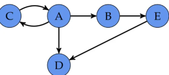
unique, which makes it trivial to construct an unique edge labeling for simple graphs by combining the vertice labels; this applies also for directed simple graphs with edges oriented in both directions between vertice pairs. A small, labeled, directed graph can be seen in Figure 1.

Edges of a graph link its vertices together: an edge (u,v) is said toconnectvertices

uand v. A path in an undirected graph G is a sequence of edges (e1,e2, . . . ,en),

∀_e_i ∈_E₍_G_),_i∈ {₁,₂, . . . ,_n}_{, which connects a sequence of vertices (}_v₁,_v₂, . . . ,_v_n,_v_n₊₁_),

where∀_v_i ∈ _V₍_G_{), and}_e_j = ₍_v_j,_v_j₊

1),j ∈ {1,2, . . . ,n}. Similarly as in the case of a

single edge, the vertices along the path are said to beconnected. The length of a pathp,len(p), is the number of edges it contains. Furthermore, we say that the (directed) distance between the verticesuandvin a graphGis the length of the

(11)

A B C

D

E

Figure 1: A small directed graph, with five labeled vertices and six unlabeled edges.

shortest path,ps₍_u,_v_{), between}_u_and_v _{in the graph}_G_{. The shortest path from}

vertice to itself has zero length,len(ps₍_u,_u₎₎₌_{0 for all}_u_∈_V₍_G_{). If there is no path}

fromutov, thenlen(ps₍_u,_v₎₎₌_∞_.

3.2 Call Graphs

In this section we introduce call graphs. We start by defining overall characteristics of call graphs and move on to issues and matters more focused to this thesis.

A call graph of a program is a labeled directed graph, which represent the caller-callee relationships of the program’s functions. A call graph can be constructed either by using behavioral or static analysis. In the former case, the call graph is obtained at runtime by analysing program’s behavior in a sandbox environment, and in the latter, by running a disassembler on the program’s binary.

The call graphs obtained by the behavioral analysis tend to obtain only partial information of the caller-callee relationships, since all calling routines are not necessarily observed during a finite number of runs or a limited amount of runtime. On the other hand, they may capture sequential control flow information, which may prove to be essential in defining exact behavioral traits of the program. Static analysis collects more thorough information of the program binary’s structure, but may end up being largely redundant, e.g. in the case where several large common libraries have been included in the binary, but very few of their individual functions have been called. Furthermore, the static analysis tools may be unable to decide which exact function is called from the function set, and therefore can leave some possible call structures unnoticed.

Call graphs can be eithercontext sensitiveorcontext insensitive. Context sensitive call graphs add an additional vertex for every call configuration (e.g. parameter configuration) that is used to call the function. Context insensitive call graphs add only one vertex for all configurations. Call graps discussed in this thesis are

(12)

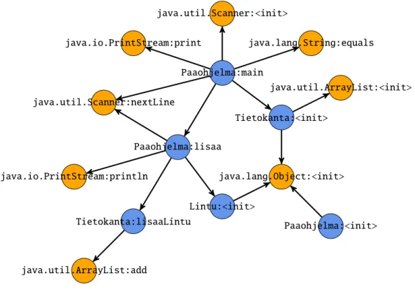
Paaohjelma:main Tietokanta:<init> Paaohjelma:lisaa Tietokanta:lisaaLintu java.util.Scanner:<init> java.io.PrintStream:println java.util.Scanner:nextLine java.lang.String:equals java.lang.Object:<init> java.io.PrintStream:print java.util.ArrayList:add java.util.ArrayList:<init> Paaohjelma:<init> Lintu:<init>

Figure 2: An example of a small call graph extracted from a Java program. The orange nodes with methods starting with ‘java’ are library (non-local) functions, and the blue nodes are user defined (local) functions.

context insensitive. An example of call a graph structure can be seen in the Figure 2. Typically, extracted call graphs are heavily tree like with a root in a program’s entry point, e.g. themain_{-method of a Java program’s main class. However, due}

to multiple reasons (some of which are elaborated in the Section 3.4), they can contain areas not connected by the call structure, or even singular nodes with no incoming or outcoming calls.

The call graph’s vertice set can be divided between different kind of functions: local (user defined), common library, external and thunk functions; the latter three called together as non-local functions. In this thesis, only the difference between local and non-local functions is considered. This partitioning is done because, at compile time, the compiler can alter the names of the local functions inside the binary, but the names of the non-local functions remain the same.

Since there is a one-to-one match between program functions and call graph vertices, all the vertices can be uniquely labeled based on the name of the function they represent.3 _{Moreover, on similar platforms, matching non-local function}

(13)

names generally point to the same function, making it possible to partially label and match the functions between different call graphs based on non-local function names.

Definition 4 (Call graph). A program’s call graph is a labeled directed graph defined by 5-tuple G = (V(G), E(G), L, L, _T_{), where} _V₍_G_{) is the set of vertices}

each representing a single function in a program;E(G) is a set of directed edges where (u,v)∈_E₍_G_{) marks that there is a call from function represented by}_u_{to a}

function represented byv;L_{is a set of possible labels, e.g. program’s function}

names;L: V(G) → L_{is a labeling function that assigns an unique label to each}

vertex; T : V(G) → {L,_N} _{is a function that assigns a type for each vertex, L}

means that corresponding function in the program is local and N that it is non-local. Moreover, we will denote the set of all local functions in a call graphGby

VL(G)={v|v∈V(G) : T(v)=L}, and similarly the set of all non-local functions by

VN(G)={v|v∈V(G) :T(v)=N}.

It is important to notice that in our definition a single call graph isfullylabeled, but when we are dealing with a set of call graphs we treat them aspartiallylabeled. Each call graphGin a call graph set is partially labeled so that the set of non-local functions,VN(G), is labeled, and the set of local functions,VL(G), is not. The need

for this change arises from the fact that the local function names can be heavily altered in the compiling phase, and should not be trusted to have any real meaning. The names of the non-local functions on the other hand are not usually altered at the compiling phase, and matching non-local function names can be thought to point into the same function as mentioned earlier.

Call graphs obtained via static analysis can contain also other relevant infor-mation from the binary code. In general, it is possible to extract operational code sequences for each local function in the binary. These sequences can be used to create control flow graphs (CFG) of the local functions. Control flow graph of a function represents all the possible paths the function’s basic block structure can be traversed and the jump points to other basic blocks inside the function or to the entry points of other functions. However, we restrict ourselves to only consider caller-callee relationships, and no additional information of the local functions’ inner structure is used.

from function calls to call graph edges, we will make no distinction between nodes and underlying functions and may refer to nodes as functions and directed edges as calls.

(14)

3.3 Graph Similarity Measures

Graph similarity measures try to define, or approximate, how similar two graphs

GandHare. Various graph similarity measures have been proposed for different purposes. The main approaches that have been used with call graphs are: ap-proximate graph edit distance (GED), maximum common subgraphs (MCS), and matching functions based on local neighborhoods and control flow graphs.

Graph edit distance [31] is a derivation of the Levenshtein (or edit) distance for sequences [21]. It is obtained by computing how many alterations have to be done to graphGfor it to become isomorphic with graphH. Next, we will give more formal definition of graph edit distance.

Definition 5(Graph edit distance). Graph edit distance between labeled graphsG

andHis a minimum cost elementary operation sequence which transforms graph

Ginto graphH, where each of the elementary operations is assigned a certain cost. For labeled graphs, elementary operations included are vertex and edge relabeling, deletion and addition. In a basic situation, all operations have a fixed cost of 1.

As determining graph isomorphisms is neither known to be solvable in polyno-mial time nor NP-complete [14], GED is usually approximated via some method. Kinable [16] uses simple relabeling cost which is improved with simulated anneal-ing in [17].

Maximum common subgraph techniques try to find maximal subgraphgthat is contained in both graphs. Finding a subgraph that is isomorphic with graphg

from a graphGis known to be NP-complete problem [8]. Therefore maximum common subgraph techniques tend to become slow as the graph sizes increase.

Definition 6(Maximum common subgraph). Maximum common subgraph be-tween graphsGandH, is the subset of vertices inG, g ⊆_V₍_G_{), for which there}

is a bijection to a subset of vertices inH,h⊆_V₍_H_),_g_{is isomorphic to}_h_{, and}|_g|_is

maximal.

Function matching concentrates on optimizing a mapping of nodes from graph

Gto graphH. In call graphs they usually use local functions’ control flow graph information to enhance the mapping algorithm (see, e.g. Carrera and Erdélyi [6]). However, each implementation uses their own heuristics; making this approach more diverse than the other two.

(15)

3.4 Code Obfuscation

Code obfuscation techniques are used by malware authors in order to hinder the detection of their malware by antivirus software, and once captured, the analysis of the malware’s binary code. Obfuscation can be made beforehand, e.g. with packers [29], or it can happen during the malware’s life in the wild by self-mutation [5]. Next, we will take a short look on some of the obfuscation techniques that can alter the structure of statically analysed call graphs. Interested readers can see e.g. [35, 33, 29] for more thorough information.

For analysts dealing with binaries, the first task is to capture the program’s binary code in order to analyse the code itself. For benign programs this is easily done as static analysis techniques, like disassembly, can extract the program binary’s code by simply reading it from the binary. However, binary code extraction becomes harder for programs that can create and overwrite their code at runtime, e.g. by packing the binary code to compressed or encrypted code, which is unpacked at runtime. Packed code can be reverse engineered to resemble the original executable by unpacking, but quality of the result is depended on the exact tools used to pack – and unpack – the binary. On the other hand, malware variants that overwrite their own code cause problems for static analysis as there is no single point in time when all of the program’s code would be present in the binary [29].

Disassembly resisting malware complicates capture of the code structure in static analysis. Malware variants can have significant proportions of their codebase consisting of hand-written assembly code with irregular structure. They can hide code, corrupt the code analysis with non-code bytes, or even try to find errors in disassemblers by stress testing them with large quantities of exceptional inputs. Effectiveness of these techniques rest largely at the hands of disassembly tools used.

Instruction obfuscation techniques conceal control-flow information of the pro-gram. They can, for example, simulate function calls and returns with alternative instruction sequences, use call and return instructions in non-standard way, or use indirect calls.

Self-mutating malware variants are a special case of insctruction obfuscation techniques that alter their own instructions. They can, e.g. substitute instruc-tion sets with semantically equivalent sets, permutate mutually independent instructions, insert dead-code4 into the program, change variables in semantically

(16)

irrelevant way, or alter control-flow information. However, as mutations occur directly in the machine code – and therefore in the code of malware variants themselves – they usually are rather simple. Observations have shown, that malware variants that have undergone large patches of self-mutation tend to consists of highly redundant and useless code [5]. Furthermore, call graphs are quite resistant to the code mutations, as they tend to take place locally in small patches, which do not alter the binary’s call structure.

4 Call Graph Features

Feature generation tries to find descriptive bits of information from a set of complex data points. The generated features should aid to simplify the data and represent the data well enough for meaningful analysis. The feature set can then be used, e.g. to analyse similarities between the data points or to index data points for fast retrieval from a database. The feature generation can be coupled withfeature

extractionandfeature selection; the latter being a special case of the former. Feature

exraction methods are used to reduce the redundancy and/or dimensionality of the feature set by transforming the data into a lower dimension. The feature selection is used to select a representative subset of current features as a new feature set.

When the data is represented as graphs, the most typically features generated are frequent subgraphs. They are mined by one of the many frequent subgraph mining algorithms (FSM); such as gSpan [38], MoFa [3], FFSM [13] or Gaston [24]. For a given graph setG_{and a threshold}_t_{, FSM algorithms extract all subgraphs}_g_,

which are present in at leasttgraphsG∈ G_{. However, most of the FSM algorithms}

are constructed for undirected graphs and can not handle partially labeled directed graphs, i.e. the algorithms are not build to address special properties of call graphs and their underlying generative process.

In malware analysis, the feature generation approach is more frequently applied in dynamic analysis than in static analysis. In a typical case, the interesting features are defined beforehand, and their appearance is monitored during runtime. This kind of feature generation needs expert knowledge to define the interesting features, and does not (in its simplest form) recognize other interesting behavioral patterns.

In the remainder of this section we introduce the call graph features,d-reachable

k-grams, proposed in this thesis. We begin by explaining the motivation behind the features based on some notions on how the previously used call graph similarity measures behave when underlying code is altered. Then, we present the features,

(17)

give an example how they are generated and describe their basic properties. The section ends by defining three types of values the generated features can have and how the distance between two feature sets is computed.

4.1 Motivation

The idea behindd-reachablek-grams is simple: the feature set extracted from a piece of software should exhibit similarity even though the underlying code has undergone refactoring phases which do not alter the main functionality of the code, and dissimmilarity when the functionality of the code has changed. To this extent the call graph representation is already quite robust as it is invariant of many basic refactoring techniques. However, typical call graph similarity measures, MCS and GED, are still quite vulnerable to very basic code morphing processes that alter the call graph structure.

Next, we will take a look at two of the morphing processes, which we will name aslocal distortionsandnon-local distortions. Local distortions do not change the code’s functionality but alter the call graph’s local topology. On the contrary, non-local distortions can move large patches of code to be called from another place in the program (therefore altering the call graph) and can have a substantial effect on the program’s functionality.

4.1.1 Local Distortions

Local distortions are simple code refactoring processes that do not change the code’s functionality, but alter the resulting call graph structure. Typically, they are operations that split user defined (local) functions into smaller or redundant pieces, or merge several local functions into one. The resulting call graph structure can deceive similarity measures that depend on graph edit distance or maximum common subgraphs. Example 1 introduces some local distortions and their effect on call graph structure.

Example 1(Local distortions). Consider naive Python code snippet and resulting call graph seen in Figure 3. In this example, A and B are non-local functions which can represent any imported library functions, and functions starting with L are local, i.e. they are defined in the source files.

A simple local refactoring of the code, where L1 from Figure 3 has been divided into two local functions L1 ja L2, is seen in Figure 4. Refactoring alters the call graph structure, affecting the MCS or GED between the two call graphs. Repeated

(18)

import A, B def L1 ( ) : A( ) B ( ) L1 A B

Figure 3: Original Python pseudocode and the resulting call graph

import A, B def L1 ( ) : L2 ( ) B ( ) def L2 ( ) : A( ) L1 L2 A B

Figure 4: Refactoring the original local function into two local functions. application of similar refactoring patterns can distort the call graph heavily without having any effect on code’s functionality.

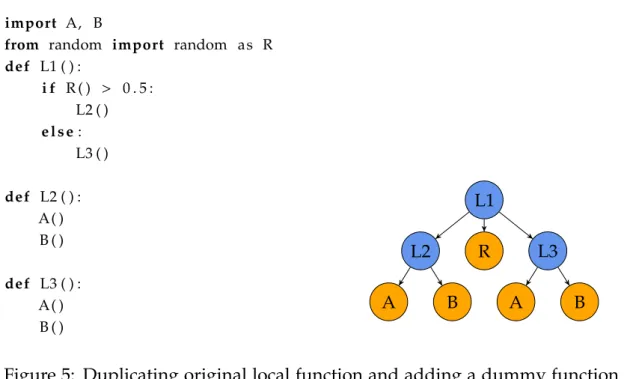
Graph edit distance is even more prone to the addition of dummy user functions with similar behaviour. This can be easily demonstrated by duplicating the original local function and choosing by random which of the equivalent functions to call, as seen in Figure 5. By replicating similar modifying process, the distance between original graph and generated graphs grows without a limit.5

4.1.2 Non-Local Distortions

On the contrary to the local distortions, non-local distortions can have a significant effect on the functionality, but can remain undetected if similarity is measured by MCS or GED. An example of a simplified non-local distortion is given in Figure 6.

Non-local distortions can include, e.g. a subprocedure involving several local functions that is first removed from the call structure and later applied into some other part of the call structure, with a distinctively different purpose. If the subprocedure itself has a single entrypoint, the GED would observe the change to be only one edge removal and one edge insertion. MCS might stay indifferent of the graph morphing process if the current MCS between the call graphs would not contain the subprocess, but also be affected if it was contained.

5_{It should be noted, that disassemblers try to capture this kind of behavior during static analysis}

(19)

import A, B

from random import random as R def L1 ( ) : i f R ( ) > 0 . 5 : L2 ( ) e l s e: L3 ( ) def L2 ( ) : A( ) B ( ) def L3 ( ) : A( ) B ( ) L1 L2 A B R L3 A B

Figure 5: Duplicating original local function and adding a dummy function to choose which one to call.

L1 L2 A B C L3 L4 D

(a) Original topology

L1 C

L3 L4

D L2

A B

(b) Topology after code transfer.

Figure 6: Simplified non-local distortion

It is important to notice, that similar graph morphing process can happen also in the case where only refactoring of the code is done without actual functionality changes. Thus, the similarity measure should (1) be able to either guess if the actual functionality has changed, or (2) be robust enough in the sense that in both situations some of the correct information is sustained. As the first option appears to be a complex (and interesting) problem by itself, and solving it reliably would probably require accessing the control flow graph information of the local functions, we choose to use the latter approach as is seen in the next section which introduces the chosen call graph features.

(20)

4.2 Definition

In this section we define the proposed features,d-reachablek-grams. We will look at the properties of the proposed features more closely in the next section.

In contrast to current methods that rely on graph matching techniques, we propose a graph distance approximation based on features that are generated

fromextended local neighborhoods, and arestructurally flavoured. The considered

extended local neighborhoods do not only cover direct child nodes, but also further descendants limited by a cutoffparameter. Structurally flavoured means, that some structural properties are taken into account when similarity between generated features are calculated, but small changes in a call graph’s call structure are not considered to change feature’s identity into another. For now, we will only consider the call graph structures that are accepted as features. We will talk more about how exact value for each feature is computed in Section 4.4.

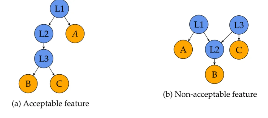
In essence, the proposed features are non-local functionk-grams that are present in a call graphG. As our call graphs have exactly one node for each function, and non-local functions between call graphs can be directly matched, we can define our features as ordered tuples of call graph node (function) labels (function names). Furthermore, because we want our features to be locally oriented and sustain some structural information, eachk-gram has to have a local function rootr, so that each non-local function in thek-gram is reachable fromr. To limit locality, we define a cutoffparameterd, so thatris connected to each function ink-gram with a shortest path at most lengthd, i.e. each function ink-gram is at mostdth successor ofr. An example of how features are accepted and rejected is given in Figure 7. Next, in Definition 7 we will give more formal definition for our features, which we named-reachablek-grams based on the cutoffparameterdand the cardinality of the feature setk, respectively.

Definition 7(d-reachablek-gram feature). Ad-reachablek-gram feature f in a call graphGis an ordered non-local function set of cardinalityk, for which there exists a local function rootr, such thatris connected to each function in f with a shortest path of length at mostd. That is, f ⊆_V_N₍_G_{) and}

f

=k, and there existsr∈VL(G), such that∀_n∈ _f _:_len₍_ps₍_r,_n₎₎_≤_d_.

As an exception, ifd=0 we don’t require any local function rootr, but instead consider only non-local function sets that are directly connected with each other6_.

6_{Remember that the set of non-local functions may also contain e.g. thunk functions that are}

used to assist calls to other functions. This leads to the fact that non-local functions can also call other non-local functions in the call graphs.

(21)

L1 L2 L3

B C

A

(a) Acceptable feature

L1 A L2 B L3 C (b) Non-acceptable feature

Figure 7: An example of how local call structure restricts feature generation. In both figures we haveVL(G)= {L1,L2,L3}andVN(G)= {A,B,C}. Lets consider

the case wherek=3, andd= 3. We can see that in Figure 7a, L1 serves as a local function root which is connected to all functions inVN(G). In Figure 7b there is no

such local function.

In essence, ifk=1 andd=0 the feature set generated is exactly the set of non-local functions, and the feature set generated with k = 2 and d = 0 would contain non-local function pairs where one is directly called by the other.

As features are mined with a bottom up procedure (see Section 5), where the

k parameter defined is the maximum cardinality of non-local function set, we differentiate single features from the whole feature set by naming our feature sets as (k,d)-grams. A (k,d)-gram of a call graph consists of alld-reachable j-grams, where j ∈ {₁,₂, . . . ,_k−₁,_k}_{. Example 2 illustrates how (}k,_d_{)-gram feature set is}

generated from a simple call graph.

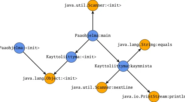
Example 2(Feature generation). As an illustrative example of the feature genera-tion, let us consider a call graph extracted from a small Java program that is shown Figure 8. We will generate the features from the call graph up tok = 5 starting fromk=1 andd=0.

The call graph,G, in Fig. 8 has four local functions,VL(G)={Paaohjelma:<init>,

Paaohjelma:main,Kayttoliittyma:<init>,Kayttoliittyma:kaynnista}and five non-local

functions,VN(G)={java.lang.Object:<init>,java.util.Scanner:<init>,

java.util.Scanner:nextLine,java.lang.String:equals,java.io.PrintStream:println}.

Now, if we generate features withk=1 andd=0, it is clear that the generated function set is the same asVN(G). When increasingkanddthe generated function

set will grow. Withk = 2 and d = 1 the only local function than can serve as a possible root for the new features isKayttoliittyma:kaynnista, because no other local

(22)

Paaohjelma:main Kayttoliittyma:kaynnista Kayttoliittyma:<init> java.util.Scanner:<init> java.io.PrintStream:println java.util.Scanner:nextLine java.lang.String:equals java.lang.Object:<init> Paaohjelma:<init>

Figure 8: An example of a small call graph extracted from a Java program. The orange nodes with methods starting with ‘java’ are library (non-local) functions, and the blue nodes are user defined (local) functions.

function combinations from the functions called byKayttoliittyma:kaynnistagives

us 3₂=

3 additional features:

• ₍_{java.io.PrintStream:println}_,_{java.lang.String:equals}_),

• ₍_{java.io.PrintStream:println}_,_{java.util.Scanner:nextLine}_{) and}

• ₍_{java.lang.String:equals}_,_{java.util.Scanner:nextLine}_).

If we increased=2, alsoPaaohjelma:maincan serve as a root, and from there all the

possible non-local function pairs are reachable whend=2. Combining the rest of the possible non-local function pairs generates 5₂₋

3=7 features more: • ₍_{java.io.PrintStream:println}_,_{java.lang.Object:<init>}_), • ₍_{java.io.PrintStream:println}_,_{java.util.Scanner:<init>}_), • ₍_{java.lang.Object:<init>}_,_{java.lang.String:equals}_), • ₍_{java.lang.Object:<init>}_,_{java.util.Scanner:<init>}_), • ₍_{java.lang.Object:<init>}_,_{java.util.Scanner:nextLine}_),

• ₍_{java.lang.String:equals}_,_{java.util.Scanner:<init>}_{) and}

• ₍java.util.Scanner:<init>_,java.util.Scanner:nextLine_).

With k = 3 and d = 1 we would only generate a single feature more:

(23)

Then, increasing d to d = 2 would generate the rest 5₃ ₋

1 = 9 of the non-local function combinations of cardinality three as all the non-non-local functions are reachable fromPaaohjelma:mainwhen d= 2, similarly as it was in the case when k=2 andd=2.

If we increasek=4, we do not generate any features withd=1 as the maximum number of non-local functions any local functions calls is three. Increasingd=2, we will then generate all the possible features with four non-local functions, giving us 5₄ =

5 features more. Lastly, ifk = 5 we do not generate any features when

d=1, and whend=2 we generate only a single feature which contains exactly the non-local function setVN(G).

4.3 Properties

We will now take a look at some of the elementary properties (and limitations) of our features, and how changes in the call graph structure affect our features. As the main focus of our features is to be invariant of small refactoring processes – and naive obfuscation techniques – that affect the call graph structure, we are mainly interested in the two refactoring processes mentined earlier: local distortions and non-local distortions.

Local distortions Local distortions affect the call graph’s topology locally, e.g by inserting more local functions, deleting them, or applying some (typically gradual) control structure changes. Our features are to some extent resilient to adding or deleting local functions, as the cutoffparameterdgives us some flexibility on how features are generated from the root function. Also, as the root function is not fixed between the call graphs, a lot of local topology changes make us simply choose another root for the feature generation, in effect keeping the generated feature set the same.

However, the feature generation is affected if local distortions are applied consecutively. For example, suppose we apply similar distortion as in the Example 1 from Figure 3 to Figure 4 many times in a row so that each local function added is inserted to be called from the local function inserted in the previous distortion. At some point inserting new local function collides with our cutoffdand feature (A,B) cannot be generated from the root L1 anymore.

Non-local distortions Non-local distortions appear in a call graph what a portion of the code is transferred to another location in the call graph. For example, let us

(24)

look at the Figure 6 where the subtree with L2 as a root is transferred to be called from L4 instead of L1. If we have defined that the cutoffparameterd=3, then any feature set generated from the subgraph shown in the image is not affected, as L3 serves as a root from which all non-local functions can be reached before and after the distortion. Same goes ford=1 as local functions’ calls to non-local functions is not changed. However, ifd= 2 we can see that in Figure 6a we can generate second order features (A,C) and (B,C), but after the code transfer in Figure 6b we generate features (A,D) and (B,D) instead.

4.4 Call Graph Distance Using Features

We now have discussed which kind of features we are interested in, and their properties. However, we are yet to cover how we can compute a distance between two call graphs based on the generated feature sets and feature values. Next, we will define the distance between call graphs. The computed distance depends on the feature values, which we will discuss after we have defined the distance measure. For now, it is sufficient to know that we denote the value of feature f in a call graphGwithvG(f). Howerer, if the call graph is clear from the context, we

may also use a shorthand notationv(f).

Definition 8(Graph distance withd-reachablek-grams). Distance between two call graphsGandH, dist(G,H), is the summed distance between their feature sets,

F(G) andF(H), respectively. More precisely, dist(G,H)= X f∈_F₍_G₎∪_F₍_H₎ vG(f)−vH(f) w(f), (1) wherevG(f) is the value of feature f in call graphG, 0≤vG(f)≤1, andw(f) is the

weight for the feature f, 0≤_w₍_f₎≤_{1, for all} _f_{. In a basic setting the weight of the}

features is constant,∀_f _:_w₍_f₎=_1.

As the distance between call graphs is the distance between their feature sets, we need define the valuevG(f) for each feature f in each call graphG. Even though

the proposed features themselves try to be resistant to small changes in the call graph topology, we can include some information about the local topology into the values of the extracted features aiming for more precise representation of the call graph. In theory, more precise representation of a single call graph should result in a more precise computation of the distance between two call graphs.

Before we give the exact formulas to compute different value types, let us consider some traits that the feature values should exhibit. Let feature f be a

(25)

d-reachablek-gram for some k > 1 and d > 0, and vG(f),vH(f) and vX(f) be the

values of feature f in call graphsG,HandX, respectively.

First, consider the case where feature is found from call graphsGandH, but not fromX. To compute the difference for the feature fbetweenG(orH) andXwe need to givef a value inX, as only computing the difference between intersecting feature sets for two call graphs is hardly a meaningful distance measure. Furthermore, the value forvX(f) must be selected in such a way that if the feature f has been

found fromGwith a smallerdthan fromH, then the difference betweenvX(f) and

vH(f) is smaller than the difference betweenvX(f) andvG(f). The reason for this

originates from a following observation: if we do not find f fromXup to certaind, we have no proof that f could not be found fromXwithd+1.

For the above mentioned reasons, we use a dummy feature value for each feature not found from a call graphG, ∀_f _* _V_N₍_G_{) :} _v_G₍_f₎ = _{0. Also, we give}

the features higher values when they are found closer to their root function by computing maximum valuemfor eachkbased on the feature value type (them

can vary between different values ofk) andd, and then use this maximum value to “flip” feature values so that the features found further away from the root (that is, non-local functions are generally further away from the connecting local function root) have values closer to zero than features found closer to the root (e.g. each non-local function is directly called by the root).

Second trait to consider is that the features of higher order (features generated with largerk) should not have larger maximum values than the features of lower order. The reason for this is simple, the higher order features would start to increasingly dominate the distance measure (remember that there is already a high change that the higher order feature set is exponentially larger compared to lower order feature set), because the difference of a single feature value could be higher between call graphs. To overcome this aspect, we use the maximum valuemfor eachkto normalize the feature values, giving us feature values that are constrained between zero and one for all call graphs and all the features. Furthermore, if the feature is generated with the exception cased=0, its value in all the feature value types is one.

Next, we will describe three types of values the generated features can be assigned to: binary, maximum distance, and sum of distances.

Binary The simplest feature value type is binary. Binary feature value represents the existence of feature f ∈_V_N₍_G_{). It is zero if the feature is not found from graph}

(26)

Gwith the givend, and one if it is found. That is, the value of feature f,vG(f), is vG(f)=          1 if f ⊆_V_N₍_G₎ 0 otherwise. (2)

Maximum distance With maximum distance as the value of a feature f in a call graphGis based to be the maximum distance between the root,r, and any non-local function in a feature. Formally, the value of feature f,vG(f), is computed

as follows: vG(f)= m( f ,d)−max{len(p s₍_r,_n₎₎_|_n_∈ _f_} d , (3)

whereps₍_·_{) is the shortest path between two functions,}_d_{is the maximum reachability}

used to generate the features, and∀_f _: _m₍ f

,d)=d+1.

Sum of distances The most complex feature value is based on the sum of distances between root and all non-local functions in the feature. Given a feature

f, we compute the value of feature,vG(f), as follows:

vG(f)= m( f ,d)− _P n∈_f len(ps(r,n)) m( f ,d)−1 , (4)

whereps₍_·_{) is the shortest path between two functions,}_d_{is the maximum reachability}

used to generate the features, and∀_f _: _m₍ f ,d)= f ×d+1.

5 Algorithm

In this section we present an example algorithm for generating (k,d)-grams from a call graph, and optional pre- and postprocessing steps. Our preprocessing step tries to minimize local distortions in each call graph, and postprocessing step is used after the features from the whole dataset have been generated in order weight the features and optionally prune some of the features. The main algorithm is implemented in a straight forward manner, and is described here only as an illustrative example of the implementation, not as a heavily optimized version of the generation process.

Next, in Section 5.1 we will first look at the preprocessing step which aims to tighten the call graph layout. Then, we move to main algorithm implementation in Section 5.2. Last, in Section 5.3 we describe some postprocessing procedures, which aim to reduce the redundancy in the collected feature set and enhance overall effectiveness of the collected features.

(27)

L1 L2

A B

C L3

D

(a) Original local topology

L1

A B C L3

D

(b) Local topology after merging.

Figure 9: Tightening the call graph topology by merging single parent local functions with their parent. The local function L2 from Figure 9a is merged into its parent L1 in Figure 9b.

5.1 Preprocessing

Although thed-reachablek-grams try to diminish the effect of the local distortions themselves, we experiment with an optional preprocessing step in order to tighten the call graph’s topology before the features are extracted. In this step, we prune away local functions that have only a single parent by combining them with their parent. An example of this procedure can be seen in Figure 9. In source code, this process has a similar meaning as defining the function to be merged as inline function.

5.2 Main Algorithm

The main algorithm for generating (k,d)-grams is simple, and can be seen to have some similarities to the frequent subgraph mining algorithms. Perhaps the most prominent difference is that the algorithm is run for each call graph separately. This can be done because we are interested inexhaustivelymining all the function sets within maximum distanced. Thus, we cannot save computation time by first mining the (k−_{1) function sets from}_all_{the call graphs in the dataset, computing}

their support, and then pruning from the feature set the features with lower support than the defined minimum support. In fact, we save computation time as only the (k−_{1)-function sets found in a single call graph are used to generate} k-function sets. This approach allows addition of new call graphs iteratively, as the minimum support of the features does not need to be adjusted.

The main body of the algorithm is described in Algorithm 1. The algorithm takes as an input a call graphGand feature generation parameterskandd, and

(28)

Algorithm 1:Main algorithm for generatingd-reachablek-grams

Input: G: a call graph

Input: k: maximum number of non-local functions in a feature

Input: d: maximum distance from root local function to non-local function

Output: generatedfeatures

1 begin

2 features←generateZeros(G, k)

3 ifk>1then

4 distances←shortestPaths(G, d)

5 collect pairs of non-local functions that have same key indistancesto

pairsand note their maximal feature value

6 features←features∪pairs

7 lastFeats←pairs

8 whilei←3tokdo

9 newFeats←generate(distances,lastFeats)

10 features←features∪newFeats

11 lastFeats←newFeats

12 i←i+1

13 collect the maximal values for each feature fromfeaturesand return them

returns the maximal value for each generated feature depending on the feature value choice (see Section 4.4 for possible feature values). The algorithm starts on line 2 by generating features for the exceptiond = 0, where the features do not have any local function root, i.e. it collects non-local feature sets where one of the non-local functions is the root and all other functions are its descendants. In line 4 it proceeds to compute (directed) distances between all local functions and non-local functions up to a cutoffdwith a slightly modified all pairs shortest path algorithm, which is introduced in Algorithm 2. The shortest path algorithm outputs a mapping from local functions to lists of pairs, where each pair contains a non-local function and the distance from the local function to the non-local function.

After generating the shortest paths, in line 5, the algorithm gathers all non-local function pairs that are at mostdth successor of some local functionrtopairs, and in lines 8–13, the algorithm iteratively increments the cardinality of the features. For each cardinalityiit uses the features generated for cardinalityi−_{1 as the starting}

(29)

and so on. The main procedure to generate the features,generate, is called in line 9, and is described in Algorithm 3. The algorithm ends by collecting the maximal value for each feature f from the generated feature candidates.7

Algorithm 2 describes how shortest paths from all local functions to non-local functions are computed with a cutoffd. The algorithm runs iteratively a slightly modified single source shortest path with a cutofffor each local function in a call graphGas the source . For each sourcel ∈ _V_L₍_G_{), it sets the target to be the set}

of non-local functionsVN(G). It outputs a dictionary where local functions are

keys and values are lists of 2-tuples. Each 2-tuple contains a name of a non-local function and the length of the shortest path to that function from the local function used as the key. The algorithm behaves exactly same as normal single source shortest path with a cutoff for each source, but instead of calculating paths to all other nodes, we set a variablenotFound to beVN(G) at the start of the loop

for each local functionrootand terminate the computation also whennotFound

=∅_{. In order to save computation time in the following generation phase, we do}

not construct full distance matrix (that is, set distances to other nodes to infinity), because then we should also process the nodes we already know we do not need to because of they are further away from therootthan the cutofffactord.

In Algorithm 3, the previously generated feature set for cardinalityiis used as a starting point to generate the feature set for cardinalityi+1. The routine takes each feature from the previous feature set into consideration and looks from which local function it has been generated asroot. Then, it looks fromdistancesall the non-local functions that ared-reachable fromroot, and combines a new feature if the function is not already in the currently considered feature. Lastly, it computes the feature’s value using the defined feature value option, and appends the feature to new feature set, which is returned at the end.

5.3 Post-processing

The post-processing step takes place after features from all call graphs have been collected. We experiment with two techniques: pruning and weighting of features.

Pruning Pruning attemps to reduce the noise in the distances computed from the feature sets by removing features that are only present in a single call graph in the dataset. These features are removed because they only add distance between 7_{In order to save computation time, this step can be done while generating the features in}

(30)

Algorithm 2: shortestPathsModified all pairs shortest paths algorithm that computes paths only from local functions to non-local functions with prede-termined cutoffd. Called from Algorithm 1 on line 4.

Input: G: a call graph

Input: d: cutoff, only distances at maxdare considered

Output: distances: a map from local functions (keys) to lists (values), where each list contains (non-local function, distance)-tuples for all

non-local functions that are at mostd-reachable from the local function used as the key.

1 begin

2 initialisedistancesto an empty map

3 forroot∈V_L(G)do

4 notFound← VN(G)

5 level←1

6 paths←{root: (root,)}

7 nextLevel←{root}

8 whilenextLevel_,∅andnotFound_,∅andlevel≤ddo

9 thisLevel←nextLevel

10 nextLevel← ∅

11 forfunc∈thisLeveldo

12 forchild∈successors(func)do

13 ifchild_<pathsthen

14 paths(child)←paths(func)+child

15 addchildtonextLevel

16 ifchild∈notFoundthen

17 deletechildfromnotFound

18 level←level+1

19 remove paths that do not end in a non-local function frompaths 20 compute the length of each path to non-local function inpaths 21 store (non-local function, length)-pairs as a list todistanceswith key

root

the graph they are in and all the other graphs. With a lot of features only present in a single graph, the effective distances may be strongly altered.

(31)

Algorithm 3: generate Routine to compute features of cardinality i from features of cardinalityi−_{1. Called from Algorithm 1 on line 9.}

Input: distances: distances from local functions to non-local functions

Input: lastFeats: (i,d)-gram features

Output: newFeats: (i+1,d)-gram features

1 begin

2 newFeats← ∅

3 forfeat∈lastFeatsdo 4 root←getRoot(feat)

5 forfunc∈distances(root)do

6 iffunc_<featthen

7 newFeat←func∪feat

8 assign a value tonewFeatbased on the chosen value type and

distances

9 addnewFeattonewFeats

Feature weighting Feature weighting aims to solve the effect of the combinatorial explosion of the number of generated features whenkincreases. With each increase inkthe feature set gets proportionally larger, as the amount of non-local function combinations increases. This raises implicitly some questions, e.g. “Which features should we be interested in?” and “Are features of order three more interesting than features of order two?”. Our answer to these questions is to limit the effect the feature set of each order has on the distance measure. We do this by weighting each feature in the generated feature set by the number of features generated for that order from all call graphs in the dataset. For example, if the number of features for the order 2 isB, then the weight for each feature f of order 2 is set to

w(f)=1/B.

6 Datasets

In our experiments we use two distinct datasets: a programming exercise dataset gathered from university students at the Department of Computer Science of the University of Helsinki, and a malware dataset obtained from F-Secure Corporation. We will call the former as the student dataset, and the latter as the malware dataset. Next, we will give a short description of the two datasets, how they were obtained, and what they consist of.