Multi-label classification of chronically ill patients with bag of words and
supervised dimensionality reduction algorithms
Stefano Bromuri
a,⇑, Damien Zufferey
a, Jean Hennebert
b, Michael Schumacher
a aUniversity of Applied Sciences Western Switzerland, Institute of Business Information Systems, TechnoArk 3, CH-3960 Sierre, Switzerland b
University of Applied Sciences Western Switzerland, Institute of Information and Communication Technologies, Bd de Pérolles 80, CH-1705 Fribourg, Switzerland
a r t i c l e
i n f o
Article history:
Received 30 October 2013 Accepted 19 May 2014 Available online 29 May 2014 Keywords: Multi-label classification Complex patient Diabetes type 2 Clinical data Dimensionality reduction Kernel methods
a b s t r a c t
Objective:This research is motivated by the issue of classifying illnesses of chronically ill patients for decision support in clinical settings. Our main objective is to propose multi-label classification of multivariate time series contained in medical records of chronically ill patients, by means of quantization methods, such as bag of words (BoW), and multi-label classification algorithms. Our second objective is to compare supervised dimensionality reduction techniques to state-of-the-art multi-label classification algorithms. The hypothesis is that kernel methods and locality preserving projections make such algorithms good candidates to study multi-label medical time series.
Methods:We combine BoW and supervised dimensionality reduction algorithms to perform multi-label classification on health records of chronically ill patients. The considered algorithms are compared with state-of-the-art multi-label classifiers in two real world datasets. Portavita dataset contains 525 diabetes type 2 (DT2) patients, with co-morbidities of DT2 such as hypertension, dyslipidemia, and microvascular or macrovascular issues. MIMIC II dataset contains 2635 patients affected by thyroid disease, diabetes mellitus, lipoid metabolism disease, fluid electrolyte disease, hypertensive disease, thrombosis, hypoten-sion, chronic obstructive pulmonary disease (COPD), liver disease and kidney disease. The algorithms are evaluated using multi-label evaluation metrics such ashamming loss,one error,coverage,ranking loss, and average precision.
Results: Non-linear dimensionality reduction approaches behave well on medical time series quantized using the BoW algorithm, with results comparable to state-of-the-art multi-label classification algorithms. Chaining the projected features has a positive impact on the performance of the algorithm with respect to pure binary relevance approaches.
Conclusions: The evaluation highlights the feasibility of representing medical health records using the BoW for multi-label classification tasks. The study also highlights that dimensionality reduction algo-rithms based on kernel methods, locality preserving projections or both are good candidates to deal with multi-label classification tasks in medical time series with many missing values and high label density. Ó2014 Elsevier Inc. All rights reserved.
1. Introduction
The average lifespan has increased considerably due to the invention of better drugs and improvement of healthcare, but the rate of chronic illnesses per patient has also increased, becoming a burden for the economy of industrialized and emerging countries [1].
The interaction between chronic illnesses and multiple drugs intake make the patient treatment complex to handle for caregiv-ers. The possibility of taking informed decisions about complex
patients is important to slow down the development of their illnesses.
Unfortunately, doctors have to take decisions whose consequences will be evaluated only after years of treatment. Furthermore, given the growth in number of chronically ill patients, caregivers are often in charge of hundreds of patients [2]. In addition, patient electronic health records (EHR) often con-tain the evolution in time of the patient clinical data, which are high dimensional multivariate time series of physiological values. As reported in[3], physicians would use services that improve their understanding of an illness even if these involve more cognitive effort than in the standard practice. In particular, in the medical informatics and data mining community [4,5] it has already been discussed that classifying patients given their http://dx.doi.org/10.1016/j.jbi.2014.05.010
1532-0464/Ó2014 Elsevier Inc. All rights reserved. ⇑ Corresponding author.
E-mail address:[email protected](S. Bromuri).
Contents lists available atScienceDirect
Journal of Biomedical Informatics
physiological values and laboratory tests may help caregivers’ decision making process.
This paper is motivated by the problem of classifying patients affected by multiple illnesses to enhance the decision support of medical doctors. There are two challenges to overcome in order to define a system capable to correctly classify the multiple illnesses that may affect a chronically ill patient: (a) dealing with irregular multivariate time series; and (b) dealing with the interac-tion of multiple co-morbidities in a heterogeneous populainterac-tion of patients.
The presence of high dimensional and multivariate data presents a big challenge to standard classification algorithms due to the curse of dimensionality [6]. Clinical time series are often irregular, a patient may present different number of records with respect to another patient and the periods of time in which the val-ues are collected may not be aligned. The challenge is even more difficult if we consider the inherently multi-label properties of medical data, where a patient may present multiple co-morbidities at once.
Concerning irregular time series, quantization algorithms, such as the Bag of Words (BoW) model, have proven successful in sev-eral medical tasks[7].
As a matter of fact, BoW is often used in biomedical time series. In[7], Wang et al. present an application of the BoW model to EEG and ECG signals. Similarly to us, the authors of[7]are faced with the issue of time series of different length with possibly heteroge-neous patients at hand.
Jiu et al. present a supervised approach towards BoW codebook generation using neural networks in[8]. In particular, the approach uses Multi-Layer Perceptrons (MLP) and the backpropagation algorithm to update the weights of the codewords according to their discrimination capabilities with respect to a set of classes.
Similarly to[8], in[9]Ordonez et al. present a modification of the BoW model to classify medical time series. Such a model uses continuous multivariate time series to compute a symbolic repre-sentation of the signals that is then used as the codebook for the classification of the patients.
Concerning multi-label classification algorithms, an extensive review can be found in [10]. Multi-label learning [11] implies training sets where each instance has a labelset and the task is to predict the labelset of unseen instances. As reported in[10], there exist works that combine supervised dimensionality reduction with multi-label learning [12–14]. Furthermore, most of these works focus on applying multi-label techniques on text analysis with static datasets[15].
In general terms multi-label classification of complex patients in discrete medical time series is quite an unexplored issue. Firstly, we think that the main contribution of this paper is to propose the combination of BoW, to quantize irregular time series present in patient health records, and multi-label classification algorithms, to classify the chronic illnesses that a patient may present. These are two established techniques, but in medical settings their com-bination is quite novel.
Secondly, we believe that this contribution is interesting to biomedical informatics as we evaluate linear and non-linear super-vised dimensionality reduction approaches with respect to multi-label classification in medical time series, and we compare these approaches with state-of-the-art multi-label classification algo-rithms. In doing this, we aim at identifying the most effective supervised dimensionality reduction techniques with respect to medical time series. We aim to confirm the hypothesis that, given the nature of the data at hand, non-linear supervised dimensional-ity reduction algorithms have a behavior comparable to state of the art multi-label classifiers.
Thirdly, our contribution is also of interest to biomedical research because we perform our evaluation against two real
world medical datasets: the Portavita dataset, provided for this study by the Portavita company,1containing 525 diabetic patients
presenting, sometimes simultaneously, hypertension, dyslipidemia or microvascular and macrovascular complications of diabetes type 2 (DT2)[16]; an extraction of 2635 patients from the public MIMIC II database[17], where we consider patients affected simultaneously by thyroid disease, diabetes mellitus, lipoid metabolism disease, fluid electrolyte disease, hypertensive disease, thrombosis, hypoten-sion, chronic obstructive pulmonary disease (COPD), liver disease and kidney disease.
The rest of this paper is organized as follows: Section2presents a background on multi-label classification, kernel methods, and supervised dimensionality reduction algorithms; Section 3 pre-sents the Portavita and MIMIC II datasets and their properties; Sec-tion4presents the training schema for the attempted multi-label classification algorithms; Section5presents an evaluation for the multi-label algorithms considered in this paper; finally, Section6 concludes this paper and draws the lines for future work.
2. Background
In this Section we present the concepts of multi-label classifica-tion, kernels, locality preserving projections and multi-class Fisher discriminant analysis. In Section4 we show how we combined these concepts in a system for classification of multi-label chroni-cally ill patients.
2.1. Multi-label classification
LetXbe the domain of observations and letLbe the finite set of labels. Given a training set T¼ fðx1;Y1Þ;ðx2;Y2Þ;. . .; ðxn;YnÞg ðxi2X;Yi#LÞi.i.d. drawn from an unknown distribution D, the goal is to learn a multi-label classifierh:X!2L. However,
it is often more convenient to learn a real-valued scoring function of the formf:XL!R. Given an instancexi and its associated
label setYi, a working system will attempt to produce larger values
for labels inYithan those that are not inYi, i.e.fðxi;y1Þ>fðxi;y2Þ for anyy12Yi andy2RYi. By the use of the function fð;Þ, we
can obtain a multi-label classifier: hðxiÞ ¼ fyjfðxi;yÞ>d;y2Lg,
wheredis a threshold to infer from the training set. The function
fð;Þ can also be adapted to a ranking functionrankfð;Þ, which
maps the outputs offðxi;yÞfor anyy2Ltof1;2;. . .;jLjgsuch that
iffðxi;y1Þ>fðxi;y2Þthenrankfðxi;y1Þ<rankfðxi;y2Þ.
Furthermore, there exist several approaches to train multi-label classifiers (see[10] for a comprehensive review on the subject). The simplest approach, known asbinary relevance(BR), is to train one binary classifier per label with traditional classification algo-rithms, considering each label as a separated problem. BR has the disadvantage of not taking into consideration the relationships existing amongst labels. To overcome this issue, severalensemble methodshave been defined in the past, amongst which the most popular ones are classifier chains (CC) and label powersets
approaches (LP). CC methods work by recursively training classifi-ers with the label predicted by the previous classifier as new features. LP methods focus on training classifiers defining classes by means of subsets of the labelset. Despite having been demon-strated effective, CC and LP methods present computational disad-vantages with respect to BR methods, whose complexity is linear in respect to the number of labels. In addition, CC methods are difficult to train with classifier presenting many parameters, as each classifier in the chain needs to be optimized differently. Sec-ondly, LP method are computationally infeasible due to the large number of possible classes in a labelset.
1
Other approaches use the probabilistic distribution of the labels and their dependencies within a neighborhood to tune the classifier output. MLkNN [18]is a successful example of such a method.
Within this paper we will show the effect of using dimensional-ity reduction algorithms with a BR approach, considering the out-put of each classifier as separated, or as CC classifiers by concatenating the projected features.
2.2. Kernels
Non-linear subspaces may be suitable to describe clinical data-sets as due to their high dimensionality they may lie in complex manifolds. Therefore, we may need to map our input data in terms of clinical datasets to a higher dimensional space using a lineariza-tion funclineariza-tion. If we consider a set ofmsamplesx1;x2;. . .;xm2Rn,
belonging tocclasses, then we can consider a non-linear mapping
/:Rn! F, where we choose / so that h/ðxiÞ;/ðxjÞi ¼Kðxi;xjÞ,
whereKð;Þis a positive semi-definite kernel function.
Performing this map explicitly can be computationally expen-sive, to avoid it we can apply theKernel Trick[19], and calculate the Gram matrixKð;Þ, containing the inner product between the input vectors in the linearization space. This then allows us to modify linear techniques using the inner product with appropriate kernel functions, opening up the possibility of applying well known approaches in non-linear spaces.
Within this paper we will use the RBF kernel and thehistogram intersection kernel[20]. The RBF kernel is defined as:
Kðx;yÞ ¼exp
kxyk2
2
r
2 ð1ÞThe histogram intersection kernel can be defined starting from two histogramsxandyconsisting both ofmfeatures. We denote the ith features ofxasxiand foryasyi. Then we can define the kernel as:
Kðx;yÞ ¼X m
i
minðxi;yiÞ ð2Þ
A big advantage of this kernel is that it is parameterless.
2.3. Locality preserving projections
As explained in[21], a LPP projection is a linear transformation for which the data residing in a spaceRnare mapped in a subspace
Rr, with r<n, such that nearby data pairs in the original
n-dimensional space are also close in the identified subspace. More formally, if we consider a square matrixA2Rdd, whereA
i;j2 ½0;1,
representing the affinity between the elements xi and xj in a
dataset with delements, the TLPP transformation matrix can be
defined as follows: TLPP¼arg min T2Rdr 1 2 Xn i;j¼1 Ai;jkTTxiTTxjk2 ! ð3Þ
Within this paper we are interested in the usage of such a projec-tion within the KLFDA technique, further details on how to calculate
TLPPcan be found in[21].
2.4. Linear discriminant analysis and local linear discriminant analysis
Linear Discriminant Analysis (LDA)[22]is a widely used super-vised dimensionality reduction technique that can find the linear transformation which best separates elements of different classes. To achieve this, LDA makes use of the within-class scatter matrix
SðwÞ and of the between-class scatter matrix SðbÞ. These can be defined as: SðwÞ¼X C i¼1 X x2Ei ðx
l
iÞðxl
iÞT ð4Þwhere
l
iis the mean of classEi, andSðbÞ¼X C
i¼1
Nið
l
il
Þðl
il
ÞT ð5Þ wherel
is the global mean and Ni is the number of elementsbelonging to class Ei.SðwÞ is a measure of the variance between
the elements belonging to the same class, whileSðbÞis a measure of the variance of the elements belonging to different classes. Ideally, we want the scatter to be minimized for elements of the same class and maximized for elements of different classes. The transformation matrixTLDAthat achieves this is defined as:
TLDA¼arg maxdetðT
T SðwÞTÞ detðTTSðbÞT
Þ ð6Þ
As explained in[23], to specify a Locality Sensitive LDA (LSDA), we can define the local within-class scatter matrix eSðwÞ and the local between class scatter matrixeSðbÞ
e SðwÞ¼1 2 Xn i;j¼1 f WðwÞ i;j ðxixjÞðxixjÞ T ð7Þ e SðbÞ¼1 2 Xn i;j¼1 f Wði;bjÞðxixjÞðxixjÞ T ð8Þ where f WðwÞ i;j ¼ Ai;j=Ni ifyi¼yj¼c; 0 ifyi–yj ( ð9Þ f WðbÞ i;j ¼ Ai;jð1=N1=NiÞ ifyi¼yj¼c; 1=N ifyi–yj ( ð10Þ which implies that we are weighting the pairwise values according to their affinity matrixAi;j2 ½0;1, withAi;jcloser to 1 ifxjis close to xiand to 0 if they are far apart.
Then, the objective function can be expressed again as a generalized eigenvalue problem:
TLSDA¼arg max T2Rdr
trððTTeSðwÞTÞ1TTe SðbÞTÞÞ
h i
ð11Þ we refer the interested reader to[23], for further details on how to compute LSDA.
2.5. Kernel local Fisher discriminant analysis
KLFDA[23]is a generalization of the previously presented LSDA using kernel functions. If we consider eS/
b;eS / w andeS
/
t as the local
between-class, within-class and total scatter matrices respectively in the space identified by a kernel mapping, then KLFDA seeks to find:
Topt¼arg maxT
TeS/ bT TTeS/wT¼arg max TTeS/ bT TTeS/ tT ð12Þ We can justify the use of supervised techniques based on LPP and kernel methods with the considerations in[21], for which LPP is particularly useful in applications where by preserving the struc-ture of the neighborhood in the lower dimensional space, nearest neighbor based approaches can still perform well, and the curse of dimensionality is mitigated. Kernel methods are useful in cases where the classes are non-linearly separable. In our case, we apply the version of KLFDA specified in[23]using regularization.
3. Materials
In this Section, we present the descriptive statistics of the two datasets taken into consideration. For multi-label datasets, amongst the descriptive statistics it is important to also consider
label cardinalityandlabel density. Given a datasetD, and a set of labelsL, where the labels of an example are denoted withYi we
can define label cardinality and label density as below.
Label Cardinality:Label cardinality of a datasetDis the average number of labels of the examples inD:
LCðDÞ ¼ 1 jDj
XjDj
i¼1
jYij ð13Þ
Label Density: Label density ofD is the average number of labels of the examples inDdivided byjLj
LDðDÞ ¼ 1 jDj XjDj i¼1 jYij jLj ð14Þ
Label cardinality quantifies the average number of alternative labels that characterize the examples in the dataset. With respect to label cardinality, label density also considers the number of labels. The two metrics are important because multi-label algorithms may present a different behavior in datasets with similar cardinality, but different density.
3.1. The Portavita dataset
The Portavita dataset is a medical dataset collected during the standard care of DT2 patients. Such a dataset includes 525 diabetic patients affected by four complications which are: hypertension, dyslipidemia, microvascular and macrovascular diseases. A summary showing the distribution of the labels amongst the patients in such a dataset is shown inTable 1.
The Portavita dataset presents a label cardinality of 2.13, a label density of 0:532, with a total of 15 possible symbols (combination of co-occurring labels), all occurring in the dataset. All patients have multiple health records (>3), for an average number of records per patient equal to 6:72 and a total number of records equal to 3528, comprising a set of common laboratory tests and physical examinations that are part of normal routine tests in DT2.Table 2gives a summary of the descriptive statistics of such laboratory tests.
Depending on the stability of the diabetic patient physiological values, the data may be collected once every six months, or once every three months, to check for the presence of microvascular or macrovascular complications.
As this is a real world dataset, the presence of a label may simply point towards a suspected issues, requiring further labora-tory tests before it can be confirmed. In other cases, the label is assigned at the beginning of the treatment, and then it is never removed even if the patient does not present the complication any more.
We can calculate that the prior probability for a patient to present a label to be 53.33% for each label, which represents a base average precision to compare against with the attempted
classifiers. In the Portavita dataset, the tests are performed with a frequency of 3/6 months for most of the features, which are conducted at the same time for each patient, and consequently, it is quite easy to produce a set of vectors and to go from the relational model to the multivariate time series associated to a patient for this dataset.
3.2. MIMIC II dataset
As a second dataset for our study, we decided to use an extrac-tion of 2635 patients from the MIMIC II database. Since MIMIC II is a large database, we decided to select patients that had more than 40 records. Our selection has an average of 60:39 records and a total of 159,127 records. The chronic illnesses and number of patients per illness in MIMIC II dataset are shown inTable 3.
The MIMIC II dataset has a label cardinality of 2:54 and a label density of 0:254, with 1023 possible symbols, of which 194 are present in the dataset. The patients of MIMIC II are very different from those of Portavita, as MIMIC II is focused on intensive care patients, while Portavita’s patients are standard care patients. This also implies that there are more laboratory tests collected per patient in MIMIC II than in Portavita.
In MIMIC II the frequencies of the laboratory tests depend on the gravity of the patient and not on a treatment. We transformed the patients’ records in multivariate time series by taking the sam-ple frequency of the most frequent laboratory tests for each patient (for example, glucose in serum) and we applied a last observation carried forward (LOCF) to the less frequent measurements consid-ering them as constant between two measurements. We are aware that LOCF underestimates the variability of the data. Our simplify-ing assumption in applysimplify-ing LOCF is that if the variability between measurements of such values was not crucial for the caregivers of the intensive care units in the first place, then it is acceptable to underestimate variability in our classification analysis. Validating approaches to handle data sampled with different frequencies is an interesting problem that we cannot exhaust within a single con-tribution, and therefore will be subject of future work.
For those data that are completely missing, we applied the imputation approach explained in the next Section.
The descriptive statistics of MIMIC II dataset, are shown in Table 4. In MIMIC II case, the descriptive statistics for the physio-logical values are calculated before the LOCF procedure. The miss-ing values rates are calculated after LOCF. A difference between Portavita and MIMIC II datasets is that Portavita has a balanced dis-tribution of labels, whereas in MIMIC II the patient populations are imbalanced. Additionally the two datasets differ in label density. Another difference is that Portavita has a time granularity of months, whereas the tests are performed multiple times per day in MIMIC II. Finally, Portavita has way more missing values than MIMIC II. These differences will allow us to evaluate the considered algorithms in diverse settings and thus also highlight their strengths and weaknesses.
3.3. Missing value imputation
For both of the datasets, the multivariate time series present missing values. In medical datasets, the missing at random assumption does not hold, since if a patient presents missing val-ues for a test, it is often because there was no medical reason to perform it. Thus, removing patients with many missing values would bias the study towards patients with more recognized med-ical conditions. Similarly, removing features with many missing values implies losing information about the status of the patients. In the Portavita dataset, some of the features are missing more than 90% of the values. This is quite a normal situation in real world standard care datasets, as the patients considered may have
Table 1
Distribution of labels in the Portavita dataset.
Label Number of patients %
Hypertension 280 53.33
Dyslipidemia 280 53.33
Microvascular 280 53.33
different treatments and needs. To be useful, classification algo-rithms must be robust to large amounts of missing values and still be able to generalize with respect to unseen data.
It is well known that there is not a single universal approach to deal with missing values[24]in medical datasets. One of the most used approaches is to substitute the mean for the missing values [25], but this is rarely considered acceptable[26]. A more accept-able approach is to use medical knowledge to substitute with val-ues within a likely range [26]. With respect to the mean imputation, this avoids the misleading effect of considering ill someone due to imputing values out of normal ranges.
Given these considerations, we performed plausible physiolog-ical values imputation in our multi-label classification analysis. We either impute physiological values in ranges that are likely for the given patient illnesses (putting high blood pressure if the patient has hypertension) or we impute physiological values of a healthy person when the related illness label is absent (normal blood pres-sure if the patient has not hypertension).
4. Methods
In this section we illustrate how we apply a set of multi-label classification algorithms to the selected medical discrete time series datasets.
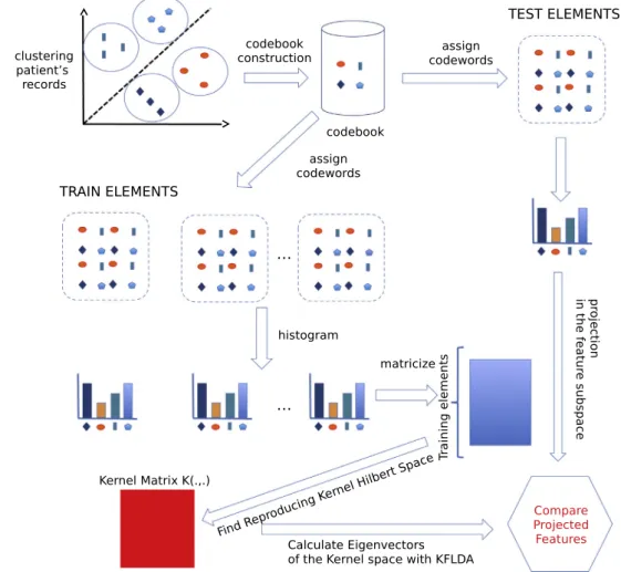
For each of the algorithms selected we apply the following steps on the data: after transforming our data from medical records to multivariate time series as described in Section3, we standardize the data to have the same contribution for each feature, we apply a BoW quantization and we standardize the data again to have the same contribution for each codeword. Then, for dimensionality reduction approaches, we apply a dimensionality reduction algorithm and we use a nearest centroid classifier based on the cosine distance. For standard multi-label classifiers, we apply the multi-label classification algorithm after the second standardiza-tion step. Fig. 1, inspired by the work of Wang et al. in [7], illustrates the main steps applied by our system in the specific case of KLFDA. For the comparison, we chose the following algorithms, all applied on the model calculated with BoW:
BoW Cosine: This technique applies the cosine distance on the patient histograms and it represents the baseline for the comparison.
LDA-BR, KDA-BR and KLFDA-BR: Linear Discriminant Analysis [27], Kernel Discriminant Analysis and Kernel Local Fisher Discriminant Analysis, with a binary relevance approach, where the classes of the patients are those explained in Section3. LDA, KDA and KLFDA: The same as above, but concatenating the
features.
MLkNN, DMLkNN, BPMLL, BR-SVM: Multi-label k-nearest neighbors [18], dependent multi-label k-nearest neighbors [28], back propagation multi-label learning[29]and multi-label support vector machines with a binary relevance approach[30]. We purposely decided to use multi-label algorithms capable of handling non-linearly separable data to confirm our hypothesis that supervised dimensionality reduction algorithms such as KLFDA and KDA are suitable candidates for multi-label learning in medical time series. In the rest of this Section we explain how we apply the BoW algorithm, the nearest centroid classifier and finally the metrics used for the evaluation of the multi-label classifiers.
Table 2
Portavita dataset descriptive statistics.
Test name Frequency MEAN MEDIAN MIN MAX SD % Missing values
BMI (kg/cm2
) Each visit 29.79 29.00 16.00 49.00 5.20 0.00
Body Weight (g) Each visit 85.17 84.00 35.00 189.00 16.99 0.00
Heart-rate (bpm) 3/6 months 72.83 72.00 60.00 360.00 11.26 35.44
Height (cm) Once 169.04 169.00 130.00 270.00 9.95 52.33
Abdominal circumference (cm) 3/6 months 103.03 102.00 75.00 189.00 13.57 84.17 Diastolic blood pressure (mmHg) 3/6 months 78.24 80.00 60.00 180.00 9.81 7.61 Systolic blood pressure (mmHg) 3/6 months 138.07 138.00 100.00 270.00 17.69 7.90
HDL-cholesterol (mg/dL) 3/6 months 1.22 1.20 0.09 9.30 0.34 2.58
LDL-cholesterol (mg/dL) 3/6 months 2.72 2.60 0.30 17.20 0.98 5.09
HbA1c (mg/dL) 6 months 52.29 50.00 5.30 180.00 12.91 16.27
Total Chol/HDL-Chol ratio 3/6 months 4.15 3.90 1.30 27.30 1.35 4.05
Albumine/Creatinine ratio 3/6 months 5.05 1.10 0.40 939.20 18.56 49.04
Aspartate Transaminase (IU/L) 3/6 months 33.60 24.00 5.00 2985.00 71.38 91.52
Natrium (mmol/L) 3/6 months 139.73 140.00 116.00 165.00 2.84 60.26
Kalium (mmol/L) 3/6 months 4.35 4.30 2.20 7.80 0.47 39.74
Creatinine in Urine (mg/dL) 3/6 months 79.90 75.00 8.00 1085.00 29.52 18.19
Albumine in Urine (mg/dL) 3/6 months 30.81 8.00 0.60 1000.00 82.54 46.27
Hemoglobin (g/dl) 3/6 months 8.40 8.50 2.90 12.30 1.07 80.82
Fasting Glucose (mmol/L) 3 months 7.61 7.20 1.30 42.60 2.15 14.48
Alanine Transaminase (IU/L) 3/6 months 32.00 25.00 4.00 2510.00 42.81 76.53
GammaGT (IU/L) 3/6 months 61.99 35.00 4.00 2855.00 104.82 87.24
Creatinine Kinase (IU/L) 3/6 months 128.42 91.00 8.00 5750.00 176.33 92.46
Total Cholesterol (mmol/L) 3/6 months 4.80 4.70 1.30 33.30 1.16 2.55
Triglyceride (mmol/L) 3/6 months 1.94 1.62 0.12 87.05 1.49 2.84
Cockcroft (mL/min) variable 90.35 84.00 6.00 4356.00 94.03 53.32
Glucose after Meal (mmol/L) 3 months 9.03 8.20 1.20 61.00 3.68 90.68
Modification of Diet in Renal Disease (mL/min) Variable 85.02 84.00 3.00 974.00 26.29 33.29
Table 3
Distribution of labels in the MIMIC II dataset.
Label Number of patients %
Thyroid disease 297 11.2
Diabetes mellitus 875 33.2
Lipoid metabolism disease 671 25.4
Fluid electrolyte disease 1014 38.4
Hypertensive disease 1568 59.5 Thrombosis 180 6.8 Hypotension 294 11.1 COPD 573 21.7 Liver Disease 208 7.8 Kidney Disease 1013 38.4
Table 4
Mimic II dataset descriptive statistics.
Test name MEAN MEDIAN MIN MAX SD % Missing val
Hematocrit of Blood (volume fraction) 31.19 30.70 2.00 67.70 4.94 0.25
Platelets in Blood (103
/uL) 241.26 218.00 5.00 3162.00 151.43 0.27
Leukocytes in Blood (103/uL) 10.22 8.90 0.10 303.90 7.38 0.3
Hemoglobin in Blood (mmol/L) 10.51 10.30 0.00 23.80 1.70 0.3
Erythrocyte mean corpuscular volume (fL) 90.13 90.00 0.00 139.00 6.84 0.31
Erythrocytes in Blood (103
/uL) 3.51 3.45 0.00 7.39 0.61 0.31
Erythrocyte mean corpuscular hemoglobin concentration (g/dL) 33.39 33.40 0.00 39.70 1.57 0.31 Erythrocyte mean corpuscular hemoglobin (pg/cell) 30.07 30.10 0.00 46.10 2.54 0.31
Erythrocyte distribution width (Ratio) 16.07 15.60 0.00 35.00 2.34 0.32
Urea nitrogen in Serum or Plasma (mg/dL) 32.18 25.00 1.00 280.00 23.89 0.33
Creatinine in Serum or Plasma (mg/dL) 1.81 1.10 0.00 73.00 1.92 0.33
Potassium in Serum or Plasma (mg/dL) 4.18 4.10 1.40 13.80 0.67 0.61
Sodium in Serum or Plasma (mEq/L) 138.52 139.00 102.00 180.00 4.94 0.68
Chloride in Blood (mEq/L) 103.12 103.00 59.00 141.00 6.18 0.69
Bicarbonate in Serum (mEq/L) 25.41 25.00 4.00 65.00 4.97 0.69
Anion gap in Blood (mEq/L) 14.22 14.00 0.00 117.00 3.90 0.71
Glucose in Serum or Plasma (mg/dL) 130.59 116.00 4.00 2220.00 63.80 0.71
Magnesium in Serum or Plasma (mg/dL) 2.01 2.00 0.20 25.20 0.37 2.16
INR in Blood by Coagulation assay 1.74 1.40 0.00 88.60 1.47 2.71
Prothrombin time (PT) in Blood by Coagulation assay 16.89 14.60 7.00 150.00 7.09 2.74 Activated partial thrombplastin time (aPTT) in Blood by Coagulation assay 44.94 35.30 16.40 193.30 25.71 2.94
Phosphate in Serum or Plasma (mg/dL) 3.75 3.50 0.30 22.60 1.41 4.36
Calcium [Mass/volume] in Serum or Plasma (mg/dL) 8.56 8.50 0.30 25.40 0.83 4.54
pH of Urine 5.88 5.50 5.00 9.00 0.99 15.3
Urobilinogen in Urine (mg/dL) 1.79 1.00 0.20 12.00 2.61 15.3
Ketones in Urine (mg/dL) 48.93 15.00 10.00 150.00 49.13 15.3
Specific gravity of Urine by Test strip 1.02 1.02 1.00 1.08 0.01 15.3
Protein in Urine by Test strip (mg in 24 h) 106.39 30.00 15.00 500.00 146.79 15.3 Glucose in Urine by Test strip (mg in 24 h) 461.21 250.00 70.00 1000.00 401.51 15.3
4.1. From irregular multivariate time series to bag of words
The BoW model was originally introduced for text document analysis[31]. In document retrieval acodebookis defined as a set of pre-selected words, also called codewords. The BoW method counts the codewords per document, reducing each document to a histogram. Adapted versions of the BoW model have been recently applied in the field of computer vision for image classifi-cation [32,33], and for biomedical time series classification [7]. When the entities to be analyzed are not documents, but are irreg-ular time series of continuous physiological values, the codebook of the BoW model can be defined using a clustering algorithm. In this paper, thek-means algorithm[34]is used to cluster the mul-tivariate time series obtained from the health records as explained in Section3, associated to the patients to create a set of centroids. These centroids then become the codewords retained in the codebook.
More formally, if we have a set of health records
X¼ ½x1;x2;. . .;xn, withxi2Rd, wheredare numerical features of
each record, associated to a set of patientsP, where each patient can have more than one record, and a set of clustering centers
ci2 ½c1;. . .;ch calculated with k-means and representing the
codebook, then we can set an un-normalized featuref, in an un-normalized histogramu, forf¼1;. . .;jPj, as:
uf ¼X Pr
i¼1
kxicfk2 ð15Þ
wherePris the number of records associated to a patient, andk k2 is the euclidean norm. After calculatingu, we can calculate a nor-malized histogramh, as:
hf ¼ uf kuk2
ð16Þ
for f¼1;. . .;jPj. Each patient is then represented in terms of a
normalized histogram, allowing us to compare patients even if they have a different number of records.
4.2. Nearest centroid classification and label ranking
To classify a new elementxwe first use the eigenvectors com-puted with KLFDA to project the testing sample in the identified subspace for a given labelk:
^ xðkÞ¼TðkÞ
opt/ðxÞ ð17Þ
where^xðkÞis the projected testing sample using the transformation matrixTðkÞ
opt, calculated for labelk, on the mapping/ðxÞ.
Second, we concatenate all the test sample projections for each of the labels in a single vector:
^ ^
x¼ ð^xð1Þj^xð2Þj. . .j^xðkÞÞ ð18Þ
The possibility to concatenate features is a big advantage of dimensionality reduction approaches such as KDA and KLFDA as it allows us to define an easy way to chain the features calculated by the different classifiers, without the need to train another classi-fier recursively as it happens with classiclassi-fier chains (CC).
Third, we calculate acosinedistance between the mean of the projected training elements and the projected testing element for each of the labels.
dk¼cosð^^x;
l
kÞ ¼ ^ ^ xl
kk^^xkk
l
kk ð19Þwhere
l
krepresent the mean of the concatenation of the features ofthe training elements in the projected space belonging to labelk. To
decide whether an element has a label or not, we perform the following test: ^ yk¼ 1 ifdk<dk; 0 otherwise ð20Þ Finally, we can define the ranking functionrankfð^^x;kÞfor labelkas:
rankfð^^x;kÞ ¼1 dk dkþdk
ð21Þ
4.3. Multi-label metrics
As stated in [18,35], multi-label performance metrics differ from single label ones. Following the same approach presented in [36,18], we propose the following five evaluation metrics for multi-label learning.
Let a testing setS¼ fðx1;Y1Þ;ðx2;Y2Þ;. . .;ðxm;YmÞg.
Hamming loss:evaluates how many times an observation-label pair is misclassified. The score lies between 0 and 1, where 0 is the best: hlossSðhÞ ¼1 m Xm i¼1 jhðxiÞMYij jLj ð22Þ
One-error:evaluates how many times the top-ranked label is not in the set of proper labels of the observation. The score lies between 0 and 1, where 0 is the best:
oneerrorSðfÞ ¼1 m Xm i¼1
c
ðarg max y2Lfðxi;yÞÞ; ð23Þ wherec
ðyÞ ¼ 1 ify R Yi; 0 otherwise: ð24ÞCoverage:evaluates how far on average we need to traverse the list of labels in order to cover all the proper labels of the observa-tion. A score as small as possible is better:
co
v
erageSðfÞ ¼1 m Xm i¼1 max y2Yi rankfðxi;yÞ 1: ð25ÞRanking loss:evaluates the average part of label pairs that are ordered in reverse for the observation. The score lies between 0 and 1, where 0 is the best:
rlossSðfÞ ¼1 m Xm i¼1 1 jYijjðLnYiÞj jfðy1;y2Þjfðxi;y1Þ 6fðxi;y2Þ;ðy1;y2Þ 2Yi ðLnYiÞgj ð26Þ
Average precision: evaluates the average fraction of labels ranked above a particular label y2Yi which actually are in Yi.
The score lies between 0 and 1, where 1 is the best:
a
v
gprecSðfÞ ¼ 1 m Xm i¼1 1 jYij X y2Yi jfy0jrankfðxi;y0Þ6rankfðxi;yÞ;y0 2Yigj rankfðxi;yÞ : ð27Þ where M represents the symmetric difference, and n is the set-theoretic difference.5. Results
In this section we evaluate the combination of BoW and multi-label classification algorithms. In the Portavita dataset, we perform our evaluation using a leave-one-patient-out cross validation
(LOPO CV). LOPO CV proved to be suitable for the medical domain [37], as it avoids situations that happen with leave-one-out (LOO), where records of the same patient are both in the training and test-ing set. Furthermore, LOPO CV presents an advantage with respect to N-folds CV, in which the selection of the random splits may lead to choose suboptimal parameters. Given the fact that we have 525 patients and 3528 health records, the computational cost of LOPO CV is affordable for the Portavita dataset. For model selection, we split our dataset into a training/validation set and a testing set, applying a LOPO CV on the training/validation set to select the best model for the testing phase. We withheld 375 patients for the training/validation and 150 patients for the testing.
Concerning the MIMIC II dataset extraction, we used a 10-fold CV approach for the grid search, splitting the dataset and keeping 70% of the patients (1844) for training and validation and 30% (791) patients for testing, while keeping the same distribution of labels in the test dataset. 10-folds CV was chosen as this dataset counts 2635 patients for a total of 159,127 health records, and LOPO CV was computationally infeasible to run a grid search.
5.1. Parameters selection with CV
The combination of BoW and dimensionality reduction tech-niques involves many parameters: size of the codebook, neighbors for the affinity matrix, the regularization coefficient, and the num-ber of components to retain in the dimensionality reduction. Given the large amount of parameters to evaluate, we decided to run a grid search with a step of 100 for the size of the codebook, identi-fyingcb¼600 as the best size for the codebook for all the consid-ered algorithms in the Portavita dataset and cb¼800 for the MIMIC II dataset.
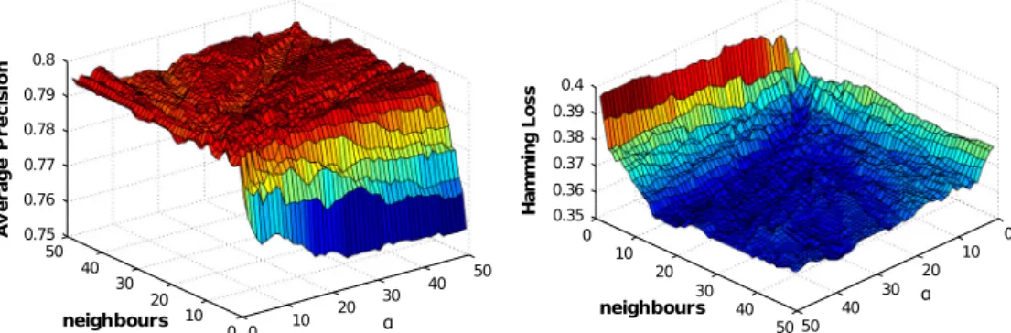
After the dimensionality reduction applied by LDA, KDA, and KLFDA, we always retain components that can explain at least 99% of the variance of the model.Fig. 2shows the grid search on average precision and hamming loss, run on the training set, for the other parameters of KLFDA in the Portavita dataset.
Table 5summarizes the parameters selection performed with LOPO CV and 10-fold cross validation concerning the algorithms studied for the Portavita and MIMIC II datasets. The parameterN
identifies the number of neighbors, whilekidentifies the regulari-zation factor,
r
the smoothing parameter for MLkNN and DMLkNN,c
the exponent of the RBF kernel, and HNthe number of hidden nodes in the BPMLL algorithm. In particular, the most difficult algo-rithm to train has been BPMLL as it requires more parameters than the other algorithms. To simplify the search, we decided to keep the learning rate constant to the default valuea
¼0:05.5.2. Results on the Portavita dataset
After training and validation of the model, we perform our test-ing ustest-ing 150 additional patients from the Portavita dataset, with
respect to the performance measures discussed in Section4.Table 6 shows the results for the selected algorithms on the Portavita data-set, with a confidence interval of 95%. The BoW Cosine approach is taken as a baseline for the comparison with the other algorithms. The classes of patients of the Portavita dataset do not appear to be linearly separable and linear techniques such as LDA and LDA-BR do not seem to improve the results with respect to a BoW clas-sifier. We think that this is due to the tendency of non-regularized LDA to overfit when the ratio between the classes and the features of the training elements is small[38,39].
KLFDA and KDA with feature concatenation achieve a better hamming and ranking loss than the other considered algorithms. KLFDA also achieves a better average precision. This suggests that in the case of classifying patients affected by DT2, the possibility of using supervised kernel methods and LPP brings an advantage in terms of classification. Another advantage of both KDA and KLFDA when compared to the other considered algorithms is the possibil-ity of concatenating the projected features calculated by each of the classifiers. The KLFDA-BR and KDA-BR algorithms, on the con-trary, do not perform much better than the standard BoW approach. In particular KDA-BR performs exactly the same as the BoW case. This is probably due to the fact that the relationship between the labels is not taken into consideration, degrading per-formances. KLFDA-BR shows an improvement with respect to BoW. This suggests that algorithms considering the locality of the data are likely to perform better than algorithms considering only the labels.
MLkNN performs similarly to KDA and KLFDA, with the best one-error score, confirming that making use of neighborhood prop-erties of the dataset is quite important in the case of DT2 patients. In contrast, BPMLL does not generalize too well with respect to new data after the training. The main issue of BPMLL is the large number of parameters to train, which makes it difficult to tune properly. Furthermore, BPMLL seems to be affected more by the large rate of missing values in the Portavita dataset than the other considered algorithms.
BR-SVM performs well in both training and testing, despite not considering the interaction between the labels, which seems to explain the difference in performance with KLFDA concerning hamming loss and ranking loss.
5.3. Results on the MIMIC II dataset
Table 7 shows the results for the selected algorithms on the MIMIC II dataset, with a confidence interval of 95%. As it is clear fromTable 7, BoW without any transformation is affected by the curse of dimensionality and LDA-BR does not really give meaning-ful results. LDA manages to improve the results with respect to BoW, but as in the Portavita dataset, the algorithm does not perform well.
First, Table 7 shows that for the MIMIC II dataset, the two best performing algorithms are MLkNN and DMLkNN, while the KDA and KLFDA algorithms perform similarly to MLkNN and DMLkNN. The fact that MIMIC II dataset has less missing values than Portavita, seems to favor the BPMLL algorithm, which performs well from the perspective of the average preci-sion. BPMLL still does not perform well for the hamming loss and the ranking loss, which we believe related to the difficulty in training the algorithm.
Second, binary relevance approaches seem to perform well on MIMIC II, except for BR-SVM. KDA-BR performs similarly to KLFDA-BR: this may happen because MIMIC II has 194 different symbols, and thus the interaction between the illnesses is quite complex, limiting the advantage of LPP projections. Furthermore, KDA-BR and KLFDA-BR seem to have comparable results to KLFDA and KDA, where the calculated features are concatenated. This may be related to the fact that MIMIC II is imbalanced. Concatenating features moves the centroid of a label depending on the features calculated for the other labels, but majority labels may have more impact in defining the centroids, degrading the performance. The difference in performance between BR-SVM, KDA-BR and KLFDA-BR is of more difficult interpretation. This could be caused by the
use of regularization or of the nearest centroid classifier in KDA-BR and KLFDA-KDA-BR algorithms.
5.4. Discussion
The fact that KLFDA and KDA perform better than the other algorithms for the Portavita dataset in respect to hamming loss and ranking loss is quite important in medical applications such as classification of diabetic patients complications. Hamming loss discriminates the capability of the algorithm to identify the presence of a complication, while ranking loss discriminates how well the algorithm ranks the labels. These metrics allow a caregiver to understand which patient illnesses have a strong expression, giving an indication on where to act more promptly.
The performed evaluation illustrates the strengths and weaknesses of KDA and KLFDA for multi-label classification tasks: the behavior of KDA and KLFDA is comparable with that of state-of-the-art multi-label classification algorithms, but they seem to present an advantage with respect to datasets with a large number of missing values and with a high label density such as the Portavita dataset. We can have a better idea of the behavior of KDA and KLFDA by looking atTable 8, comparing the hamming loss per symbol of
Table 5
Selected parameters.
Algorithm Parameters Portavita Parameters MIMIC II Interval Step
KDA-BR k¼40,cb= 600 k¼10,cb= 800 [1:50], [102:103] lin, lin
KDA k¼49,cb= 600 k¼20,cb= 800 [1:50], [102:103] lin, lin
KLFDA-BR N= 30,k¼5,cb= 600 N= 40,k¼3,cb= 800 [1:50], [1:50], [102:103] lin, lin, lin KLFDA N= 34,k¼9,cb= 600 N= 47,k¼3,cb= 800 [1:50], [1:50], [102:103] lin, lin, lin MLkNN N= 29,r¼2,cb= 600 N= 19,r¼3,cb= 800 [1:50], [1:50], [102:103] lin, lin, lin DMLkNN N= 29,r¼12,cb= 600 N= 19,r¼5,cb= 800 [1:50], [1:50], [102:103] lin, lin, lin
BPMLL k¼106
,HN= 5,cb= 600 k¼107,HN= 7,cb= 800
[108
:1], [1:20], [102:103] log, lin, lin BR-SVM C= 10,c¼101
,cb= 600 C= 5,c¼1,cb= 800 [1:102 ], [103
:103], [102:103] lin, log, lin
Table 6
Results for the Portavita dataset. Values in bold identify the best result for a given metric.
Algorithm/metric Average precision Hamming loss Ranking loss Coverage One-error
BoW 68% ± 4% 51.6% ± 4.2% 50% ± 5.6% 2.2 ± 0.14 50% ± 7.8% LDA 67.8% ± 4% 51.1% ± 4.3% 51.9% ± 5.7% 2.3 ± 0.14 48% ± 8% LDA-BR 67% ± 4% 52.8% ± 4.3% 52.2% ± 5.8% 2.3 ± 0.14 48% ± 8% KDA-BR 67.8% ± 3.8% 57.5% ± 3.2% 58% ± 3.9% 2.25 ± 0.15 48% ± 8% KDA 78.3% ± 3.8% 39.1% ± 4.1% 33.4% ± 5.5% 1.94 ± 0.16 32.1% ± 7.5% KLFDA-BR 73.5% ± 3.8% 41.6% ± 3.5% 38.9% ± 5.2% 2.07 ± 0.16 35.7% ± 7.7% KLFDA 78.8%± 3.7% 37.3%± 4% 32.2%± 5.2% 1.87± 0.16 32.1% ± 7.5% MLkNN 78.2% ± 3.7% 44% ± 3.8% 36 ± 5.5% 2 ± 0.16 30%± 7.5% DMLkNN 76.1% ± 3.8% 44.8% ± 3.8% 37% ± 5.4% 2.1 ± 0.15 33.3% ± 7.5% BPMLL 75.7% ± 3.8% 42.6% ± 4.1% 38.3% ± 5.6% 2 ± 0.16 36% ± 7.7% BR-SVM 78.2% ± 3.7% 39.3% ± 4.2% 34% ± 5.3% 1.98 ± 0.16 33.3% ± 7.5% Table 7
Results for the MIMIC II dataset. Values in bold identify the best result for a given metric.
Algorithm/metric Average precision Hamming loss Ranking loss Coverage One-error
BoW 47.5% ± 1.6% 44.5% ± 1.1% 39.5% ± 1.6% 5.6 ± 0.14 69% ± 3.4% LDA 50.9% ± 1.6% 42.7% ± 1.1% 38.2% ± 1.5% 5.4 ± 0.17 63.2% ± 3.3% LDA-BR 43.3% ± 1.4% 40.2% ± 0.8% 39.2% ± 1.4% 5.14 ± 0.15 82.93% ± 2.5% KDA-BR 64.74% ± 1.8% 23.7% ± 1.2% 26% ± 1.4% 4.67 ± 0.19 39.7% ± 3.3% KDA 66% ± 1.8% 23.4% ± 0.9% 23.2% ± 1.4% 4.2 ± 0.18 40.5% ± 3.3% KLFDA-BR 64.79% ± 1.8% 23.8% ± 1.1% 25.9% ± 1.4% 4.59 ± 0.18 40% ± 3.4% KLFDA 65.5% ± 1.8% 23.3% ± 0.9% 23.7% ± 1.4% 4.25 ± 0.16 41.1% ± 3.3% MLkNN 68.4%± 1.8% 21.7% ± 1% 20%± 1.5% 4± 0.17 35.6% ± 3% DMLkNN 68.1% ± 3.8% 21.6%± 0.8% 21.5% ± 1.5% 4 ± 0.17 34.1%± 3.2% BPMLL 67.8% ± 1% 26% ± 0.8% 37.1% ± 3.3% 4 ± 0.18 37% ± 3.3% BR-SVM 57.7% ± 1.8% 22.2% ± 0.9% 37% ± 1% 5.8 ± 0.19 38.6% ± 3.2%
KLFDA, KDA, BR-SVM and MLkNN, in the Portavita dataset (confi-dence intervals are omitted as we only have 10 elements per symbol).
In these results, we see that KDA has an advantage where the patients have only one label, which are also those patients present-ing many misspresent-ing values in Portavita dataset. For the other classes, KDA performs similarly to BR-SVM, with some exceptions, proba-bly caused by the fact that BR-SVM finds support vectors, whereas KDA is a variance based method. KLFDA seems to combine the behavior of KDA, BR-SVM and MLkNN: the eigenvectors explaining little variance are discarded just like in KDA; the use of kernel methods allows KLFDA to deal with non-linearity in the data, sim-ilarly to BR-SVM; the LPP transformation allows KLFDA to consider the neighborhood of the elements, similarly to MLkNN, but in addi-tion if there are enough elements per symbol, with a high label density, the retained eigenvectors would be able to characterize those symbols expressing most variance. In this sense, when deal-ing with datasets presentdeal-ing the three aspects of missdeal-ing data, high label density and non-linearity, KLFDA may have an advantage with respect to other techniques.
In MIMIC II, KLFDA and KDA perform slightly worse on the aver-age precision than MLkNN and DMLkNN, but they are comparable for hamming loss and ranking loss. A possible reason for this is that MIMIC II dataset is imbalanced. KLFDA and KDA are variance based methods, so an imbalanced estimation of the classes variance impacts the calculated model and its performance. Looking at the hamming loss per symbol in MIMIC II, we found that the absence of missing values in MIMIC II, cancels the advantage of KLFDA and KDA, as they behave similarly to MLkNN for patients with only one complication. Additionally, MIMIC II has a low label density, with 194 symbols and few patients for most of the symbols, which may be difficult to characterize for the variance based model calcu-lated by KLFDA and KDA. If this is the case, only the effect of the LPP projection of KLFDA, and of the nearest centroid classifier for KLFDA and KDA would be present and that would explain the sim-ilar behavior of KLFDA and KDA with MlKNN.
Finally, an advantage of KLFDA and KDA it that they compute a model based on eigenvectors, which allows to include new patients’ records by projecting their BoW representation and then recalculating the centroids for each class, while MLkNN and DMLkNN have to store the new instances in memory, that is infea-sible with big datasets.
6. Conclusions
In this paper we studied the combination of the BoW model in medical time series with dimensionality reduction approaches for
multi-label patient classification. When taking the Portavita data-set into consideration, the KLFDA algorithm with a nearest centroid classifier achieves the best results. In the MIMIC II dataset, dimen-sionality reduction algorithms are comparable to state-of-the-art multi-label classification algorithms, but suffer from the fact that the dataset is imbalanced.
There are several possible extensions to this work. At the moment we are using a single kernel mapping, but extensions of KLFDA and KDA that work with multiple kernel learning have already been defined[40]. Multiple kernels could achieve a better mapping for our data and improve the precision of KLFDA and KDA. Another promising approach could be to develop a multi-label version of KLFDA and KDA, similarly to what is proposed in[41]. This would require modifying the definition of the scatter matrices in KLFDA and KDA to consider multiple labels, which is quite a challenging problem.
In Section 3, we identified the issue of dealing with values sampled at different frequencies. Quantizing patient data with dif-ferent sampling frequencies or considering descriptive statistics rather than a codebook, could be suitable approaches. Finally, we could apply a different substitution to LOCF and generate physio-logical values with a maximum likelihood model, provided that enough patients’ records are available.
Acknowledgments
This work was partially supported by the FP7 287841 COM-MODITY12 project. We thank the anonymous reviewers for the useful comments that allowed us to improve the paper considerably.
References
[1]McAdam Marx C. Economic implications of type 2 diabetes management. Am J Manag Care 2013;19:143–8.
[2]Ghably JG, Paterson BJ, Peiris AN. Endocrinology in crisis? South Med J 2013;106:245.
[3]Kannampallil TG, Franklin A, Mishra R, Almoosa KF, Cohen T, Patel VL. Understanding the nature of information seeking behavior in critical care: Implications for the design of health information technology. Artif Intell Med 2013;57:21–9.
[4]Sun J, Sow D, Hu J, Ebadollahi S. Localized supervised metric learning on temporal physiological data. In: Proceedings of the 2010 20th International Conference on Pattern Recognition, ICPR ’10. Washington, DC, USA: IEEE Computer Society; 2010. p. 4149–52.
[5]Sun J, Wang F, Hu J, Edabollahi S. Supervised patient similarity measure of heterogeneous patient records. SIGKDD Explor 2012;14:16–24.
[6]Marimont RB, Shapiro MB. Nearest neighbour searches and the curse of dimensionality. IMA J Appl Math 1979;24:59–70.
[7] Wang J, Liu P, She MF, Nahavandi S, Kouzani AZ. Bag-of-words representation for biomedical time series classification. CoRR abs/1212.2262; 2012. [8]Jiu M, Wolf C, Garcia C, Baskurt A. Supervised learning and codebook
optimization for bag of words models. Cognitive Comput 2012;4:409–19. [9] Ordóñez P, Armstrong T, Oates T, Fackler J. Using modified multivariate
bag-of-words models to classify physiological data. In: Spiliopoulou M, Wang H, Cook DJ, Pei J, Wang W, Zaïane OR, et al. editors. ICDM workshops. IEEE; 2011. p. 534–39.
[10]Madjarov G, Kocev D, Gjorgjevikj D, Dzeroski S. An extensive experimental comparison of methods for multi-label learning. Pattern Recognit 2012;45:3084–104.
[11]Zhang M-L, Zhou Z-H. A review on multi-label learning algorithms. IEEE Trans Knowl Data Eng 2013;99:1.
[12]Ji S, Ye J. Linear dimensionality reduction for multi-label classification. In: Proceedings of the 21st international jont conference on Artificial intelligence, IJCAI’09. San Francisco, CA, USA: Morgan Kaufman Publishers Inc.; 2009. p. 1077–82.
[13]Pacharawongsakda E, Nattee C, Theeramunkong T. Improving multi-label classification using semi-supervised learning and dimensionality reduction. In: Anthony P, Ishizuka M, Lukose D, editors. PRICAI. Lecture notes in computer science, vol. 7458. Springer; 2012. p. 423–34.
[14]Qian B, Davidson I. Semi-supervised dimension reduction for multi-label classification. In: Fox M, Poole D, editors. AAAI. AAAI Press; 2010.
[15] Pestian JP, Brew C, Matykiewicz P, Hovermale DJ, Johnson N, Cohen KB, et al. A shared task involving multi-label classification of clinical free text. In: Proceedings of the workshop on BioNLP 2007: biological, translational, and
Table 8
Hamming loss per symbol in the Portavita dataset. H = Hypertension, D = Dyslipidemia, Mi = Microvascular, Ma = Macrovascular. Symbol H D Mi Ma KLFDA (%) KDA (%) BR-SVM (%) MLkNN (%) 1 No No No Yes 40 42.5 60 60 2 No No Yes No 40 35 47.5 50 3 No No Yes Yes 40 45 42.5 42.5 4 No Yes No No 25 32.5 27.5 40 5 No Yes No Yes 42.5 45 40 42.5 6 No Yes Yes No 20 15 15 30
7 No Yes Yes Yes 40 40 42.5 42.5
8 Yes No No No 35 32.5 40 45
9 Yes No No Yes 40 40 45 57.5
10 Yes No Yes No 47.5 57.5 47.5 42.5
11 Yes No Yes Yes 45 40 62.5 52.5
12 Yes Yes No No 27.5 40 20 40
13 Yes Yes No Yes 40 40 40 42.5
14 Yes Yes Yes No 35 37.5 30 30
clinical language processing, BioNLP ’07, association for computational linguistics. Stroudsburg, PA, USA; 2007. p. 97–104.
[16]Cade WT. Diabetes-related microvascular and macrovascular diseases in the physical therapy setting. Phys Ther 2008;88:1322–35.
[17]Saeed M, Villarroel M, Reisner AT, Clifford G, Lehman L-W, Moody G, et al. Multiparameter intelligent monitoring in intensive care II (MIMIC-II): a public-access intensive care unit database. Crit Care Med 2011;39:952–60. [18]Zhang M-L, Zhou Z-H. ML-KNN: a lazy learning approach to multi-label
learning. Pattern Recognit 2007;40:2038–48.
[19]Shawe-Taylor J, Cristianini N. Kernel methods for pattern analysis. Cambridge University Press; 2004.
[20] Barla A, Odone F, Verri A. Histogram intersection kernel for image classification. In: ICIP (3). p. 513–16.
[21]He X, Niyogi P. Locality preserving projections. In: Thrun S, Saul L, Schölkopf B, editors. Advances in neural information processing systems, vol. 16. Cambridge, MA: MIT Press; 2004.
[22]Fukunaga K. Introduction to statistical pattern recognition. 2nd ed. San Diego, CA, USA: Academic Press Professional, Inc.; 1990.
[23]Sugiyama M. Dimensionality reduction of multimodal labeled data by local fisher discriminant analysis. J Mach Learning Res 2007;8:1027–61. [24]Little RJ, D’Agostino R, Cohen ML, Dickersin K, Emerson SS, Farrar JT, et al. The
prevention and treatment of missing data in clinical trials. N Engl J Med 2012;367:1355–60.
[25]Dziura JD, Post LA, Zhao Q, Fu Z, Peduzzi P. Strategies for dealing with missing data in clinical trials: from design to analysis. Yale J Biol Med 2013;86:343–58. [26]Jackson D, White IR, Leese M. How much can we learn about missing data? An exploration of a clinical trial in psychiatry. J R Stat Soc Ser A Stat Soc 2010;173:593–612.
[27]Fisher RA. The use of multiple measurements in taxonomic problems. Ann Eugenics 1936;7:179–88.
[28]Younes Z, Abdallah F, Denoeux T, Snoussi H. A dependent multilabel classification method derived from the k-nearest neighbor rule. EURASIP J Adv Sig Proc 2011;2011.
[29]Zhang M-L, Zhou Z-H. Multilabel neural networks with applications to functional genomics and text categorization. IEEE Trans Knowl Data Eng 2006;18:1338–51.
[30] Cortes C, Vapnik V. Support-vector networks. Mach Learning 1995;20:273–97. [31]Ko Y. A study of term weighting schemes using class information for text classification. In: Proceedings of the 35th international ACM SIGIR conference on research and development in information retrieval, SIGIR’12. New York, NY, USA: ACM; 2012. p. 1029–30.
[32]Sivic J, Zisserman A. Efficient visual search of videos cast as text retrieval. IEEE Trans Pattern Anal Mach Intell 2009;31:591–606.
[33]Sivic J, Zisserman A. Efficient visual content retrieval and mining in videos. In: Aizawa K, Nakamura Y, Satoh S, editors. Advances in multimedia information processing – PCM 2004. Lecture notes in computer science, vol. 3332. Berlin Heidelberg: Springer; 2005. p. 471–8.
[34]MacQueen JB. Some methods for classification and analysis of multivariate observations. In: Cam LML, Neyman J, editors. Proc. of the fifth Berkeley symposium on mathematical statistics and probability, vol. 1. University of California Press; 1967. p. 281–97.
[35]Tsoumakas G, Katakis I, Vlahavas IP. Mining multi-label data. In: Maimon O, Rokach L, editors. Data mining and knowledge discovery handbook. Springer; 2010. p. 667–85.
[36]Schapire RE, Singer Y. Boostexter: a boosting-based system for text categorization. Mach Learning 2000;39:135–68.
[37]Dundar M, Fung G, Bogoni L, Macari M, Megibow A, Rao B. A methodology for training and validating a CAD system and potential pitfalls. Int Congr Ser 2004;1268:1010–4 [CARS 2004 – Computer Assisted Radiology and Surgery. Proceedings of the 18th International Congress and Exhibition].
[38] Jain A, Chandrasekaran B. Dimensionality and sample size considerations. In: Krishnaiah P, Kanal L. editors. Pattern recognition in practice; 1982. p. 835–55. [39]Linnet K. On the sensitivity of linear discriminant analysis to sampling
variation and analytical errors. Comput Biomed Res 1988;21:158–68. [40] Wang Z, Sun X. Multiple kernel local Fisher discriminant analysis for face
recognition. Signal Process 2013;93:1496–509 [Special issue on Machine Learning in Intelligent Image Processing].
[41]Park CH, Lee M. On applying linear discriminant analysis for multi-labeled problems. Pattern Recognit Lett 2008;29:878–87.