NCER Working Paper Series
NCER Working Paper Series
Forecast performance of implied
volatility and the impact of the
volatility risk premium
Ralf Becker
Ralf Becker
Adam Clements
Adam Clements
Christopher Coleman
Christopher Coleman
-
-
Fenn
Fenn
Working Paper #45
Working Paper #45
July 2009
Forecast performance of implied volatility and the
impact of the volatility risk premium
Ralf Becker*, Adam E. Clements#, and Christopher A. Coleman-Fenn#
* Economics, School of Social Sciences, University of Manchester
# School of Economics and Finance, Queensland University of Technology
July 13, 2009
Keywords: Implied volatility, volatility forecasts, volatility models, volatility risk premium, model confidence sets.
JEL Classification: C12, C22, G00.
Abstract
Forecasting volatility has received a great deal of research attention, with the relative performance of econometric models based on time-series data and option implied volatility forecasts often being considered. While many stud-ies find that implied volatility is the preferred approach, a number of issues remain unresolved. Implied volatilities are risk-neutral forecasts of spot volatil-ity, whereas time-series models are estimated on risk-adjusted or real world data of the underlying. Recently, an intuitive method has been proposed to adjust these risk-neutral forecasts into their risk-adjusted equivalents, possibly improv-ing on their forecast accuracy. By utilisimprov-ing recent econometric advances, this paper considers whether these risk-adjusted forecasts are statistically superior to the unadjusted forecasts, as well as a wide range of model based forecasts. It is found that an unadjusted risk-neutral implied volatility is an inferior forecast. However, after adjusting for the risk premia it is of equal predictive accuracy relative to a number of model based forecasts.
Corresponding author
Adam Clements
School of Economics and Finance Queensland University of Technology
GPO Box 2434, Brisbane, Qld, Australia 4001 email [email protected]
1
Introduction
Estimates of the future volatility of asset returns are of great interest to many financial market participants. Generally, there are two approaches which may be employed to obtain such estimates. First, predictions of future volatility may be generated from econometric models of volatility given historical information (model based forecasts, M BF). For surveys of common modeling techniques see Campbell, Lo and MacKinlay (1997), Gourieroux and Jasiak (2001), and Taylor (2005). Second, estimates of future volatility may be derived from option prices using implied volatility (IV). IV should represent a market’s best risk-neutral prediction of the future volatility of the underlying (see, amongst others, Jorion, 1995, Poon and Granger, 2003, 2005).
Given the practical importance of volatility forecasting (i.e. portfolio allo-cation problems, Value-at-Risk, and option valuation), there exists a wide body of literature examining the relative forecast performance of various approaches. While the results of individual studies are mixed, the survey of 93 articles com-piled by Poon and Granger (2003, 2005) reports that, overall, IV estimates often provide more accurate volatility forecasts than competing MBF. In the context of this study, Day and Lewis (1992), Canina and Figlewski (1993), Ederington and Guan (2002), and Koopman, Jungbacker and Hol (2005) report that MBF of equity index volatility provide more information relative to IV. On the other hand, Fleming, Ostdiek and Whaley (1995), Christensen and Prabhala (1998), Fleming (1998) and Blair, Poon and Taylor (2001) all find that equity index IV dominate MBF.
While there is a degree of inconsistency in previous results, the general result that IV estimates often provide more accurate volatility forecasts than competing MBF is rationalised on the basis that IV should be based on a larger and timelier information set. That is, as IV is derived from the equilibrium market expectation of a future-dated payoff, rather than on the purely historical data MBF are estimated on, it is argued that IV contains all prior information garnered from historical data and also incorporates the additional information of the beliefs of market participants regarding future volatility; in an efficient options market, this additional information should yield superior forecasts.
In a related yet different context, Becker, Clements and White (2006) ex-amine whether a particular IV index derived from S&P 500 option prices, the
V IX, contains any information relevant to future volatility beyond that re-flected in MBF. As they conclude that the V IX does not contain any such information, this result, prima facie, appears to contradict the previous find-ings summarised in Poon and Granger (2003). However, no forecast comparison is undertaken and they merely conjecture that the V IX may be viewed as a combination of MBF. Subsequently, Becker and Clements (2008) show that the
V IX index produces forecasts which are statistically inferior to a number of competing MBF. Further, a combination of the best MBF is found to be su-perior to both the individual model based andV IX forecasts. They conclude that while it is plausible that IV combines information that is used in a range of different MBF, it is not the best possible combination of such information. This research provided an important contribution to the literature by allowing
for more robust conclusions to be drawn regarding comparative forecast perfor-mance, relative to the contradictory results of prior research. This was achieved by simultaneously examining a wide class of MBF and an IV forecast, rather than the typical pair-wise comparisons of prior work, using up-to-date forecast evaluation technology.
However, prior results cannot be viewed as definitive as, aside from the inconsistency of results, it may be argued that IV forecasts are inherently disadvantaged in the context of forecast evaluation. The pricing of financial derivatives is assumed to occur in a risk-neutral environment whereas MBF are estimated under the physical measure. Hence, prior tests of predictive accuracy have essentially been comparisons of risk-neutral versus real-world forecasts; as the target is also real-world, models estimated from like data may have an ad-vantage. Without adjusting for the volatility risk premium, generally defined as the difference in expectations of volatility under the risk-neutral and physical measures, risk-neutral forecasts may be biased.
By matching the moments of model-free RV and IV, Bollerslev, Gibson, and Zhou (2008), hereafter BGZ, obtain an estimate of the volatility risk premium; it is then a straight-forward process to convert the risk-neutral IV into a forecast under the physical measure. This risk-adjusted IV can then be compared to MBF. Following Becker and Clements (2008), we conduct such a comparison us-ing the model confidence set methodology of Hansen, Lunde and Nason (2003a) and find that the transformedV IX is statistically superior to the risk-neutral
V IX in the majority of samples considered and is of equal predictive accuracy to MBF, particularly at the 22-day forecast horizon the V IX is constructed for.
The paper will proceed as follows. Section 2 will outline the data relevant to this study. Section 3 discusses the econometric models used to generate the various forecasts, along with the methods used to discriminate between forecast performance. Sections 4 and 5 present the empirical results and concluding remarks respectively.
2
Data
This study is based upon data relating to the S&P 500 Composite Index, from 2 January 1990 to 31 December 2008 (4791 observations) and extends the data set studied by Becker, Clements and White (2006) for the purposes of comparison and consistency. To address the research question at hand, estimates of both IV and future actual volatility are required. TheV IX index constructed by the Chicago Board of Options Exchange from S&P 500 index options constitutes the estimate of IV utilised in this paper. It is derived from out-of-the-money put and call options that have maturities close to the target of 22 trading days. For technical details relating to the construction of the V IX index, see Chicago Board Options Exchange (CBOE, 2003). While the true process underlying option pricing is unknown, theV IX is constructed to be a model-free measure of the market’s estimate of average S&P 500 volatility over the subsequent 22 trading days (BPT, 2001, Christensen and Prabhala, 1998 and CBOE, 2003).
Having a fixed forecast horizon is advantageous and avoids various econometric issues; hence, the 22-day length of the V IX forecast shall be denoted by Δ hereafter. While this index has only been available since September 2003, when the CBOE replaced a previous IV index based on S&P 100 options, it can be calculated retrospectively back to January 1990. It’s advantages in comparison to the previous IV index are that it no longer relies on IV derived from Black-Scholes option pricing models, it is based on more liquid options written on the S&P500 and is easier to hedge against (CBOE, 2003).
For the purposes of this study, estimates of actual volatility were obtained using the RV methodology outlined in ABDL (2001, 2003). RV estimates volatility by means of aggregating intra-day squared returns; it is important to note, as shall be discussed in more detail in the next section, that this mea-sure is a model-free estimate of latent actual volatility. It should also be noted that the daily trading period of the S&P500 is 6.5 hours and that overnight returns were used as the first intra-day return in order to capture the variation over the full calender day. ABDL (1999) suggest how to deal with practical is-sues relating to intra-day seasonality and sampling frequency when dealing with intra-day data. Based on the volatility signature plot methodology, daily RV estimates were constructed using 30 minute S&P500 index returns1. It is widely acknowledged (see e.g. Poon and Granger, 2003) that RV is a more accurate and less noisy estimate of the unobservable volatility process than squared daily returns. Patton (2006) suggests that this property of RV is beneficial when RV is used a proxy for observed volatility when evaluating forecasts.
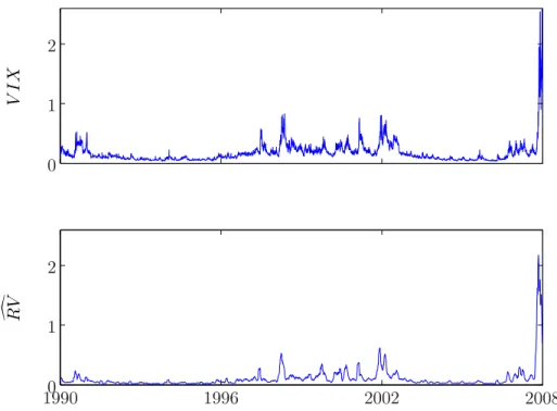
Figure 1 shows the daily V IX and the 22-day mean daily S&P500 RV,
RV = Δ1 Δi=1RVt+i, for the sample period considered. While the RV estimates exhibit a similar overall pattern when compared to theV IX, RV reaches lower peaks than theV IX. This difference is mainly due to the fact that the V IX
represents a risk-neutral forecast as opposed to RV that is a physical measure of volatility. In a perfectly efficient options market, the difference between the
V IX and actual volatility should be a function of the volatility risk-premium alone.
3
Methodology
In this section the econometric models upon which forecasts are based will be outlined, followed by how the risk-neutral forecast provided by theV IX can be transformed into a forecast under the physical measure. This section concludes with a discussion of the technique utilised to discriminate between the volatility forecasts.
3.1 Model based forecasts
While the true process underlying the evolution of volatility is not known, a range of candidate models exist and are chosen so that they span the space
VI X RV 19900 1996 2002 2008 1 2 0 1 2
Figure 1: Daily VIX (top panel) from 2/01/1990 to 1/12/2008 and 22-day mean daily S&P500 Index RV estimate (bottom panel) from 2/01/1990 to 31/12/2008.
of available model classes. The set of models chosen are based on the mod-els considered when the informational content of IV has been considered in Koopman, Jungbacker and Hol (2005), BPT (2001), and Becker, Clements and White (2006). The models chosen include those from the GARCH, stochastic volatility (SV), and RV classes.
GARCH style models employed in this study are similar to those proposed by BPT (2001). We begin with the original specification of Bollerslev (1986), where volatility is assumed to possess the following dynamics,
rt = μ+εt, εt=htzt, zt∼N(0,1) (1)
ht = α0+α1ε2t−1+βht−1
This simplest model specification is then extended to accomodate one of volatility’s stylised facts, the asymmetric relationship between volatility and returns; this extension is provided by the GJR (see Glosten, Jagannathan and Runkle, 1993, Engle and Ng, 1991) process,
rt = μ+εt, εt=htzt, zt∼N(0,1) (2)
ht = α0+α1ε2t−1+α2st−1ε2t−1+βht−1
with st−1 at unity when εt−1 < 0 and 0 otherwise. This process nests the standard GARCH model whenα2 = 0 2.
Parameter estimates for the GARCH and GJR models are similar to those commonly observed for GARCH models based on various financial time series, reflecting strong volatility persistence, and are qualitatively similar to those reported in BPT (2001)3. Furthermore, allowing for asymmetries in conditional volatility is important, irrespective of the volatility process considered.
This study also proposes that an SV model may be used to generate fore-casts. SV models differ from GARCH models in that conditional volatility is treated as an unobserved variable, and not as a deterministic function of lagged returns. The simplest SV model describes returns as
rt=μ+σtut, ut∼N(0,1) (3) whereσtis the timetconditional standard deviation ofrt. SV models treat
σt as an unobserved (latent) variable, following its own stochastic path, the simplest being an AR(1) process,
log (σt2) =α+βlog (σ2t−1) +wt, wt∼N(0, σ2w). (4)
2The conditional mean of returns is modeled as a constant. As Cochrane (2001, p 388)
points out, returns are predictable over very long horizons but at a daily frequency are virtually unpredictable.
3As the models discussed are re-estimated 3770 times in order to generate volatility
fore-casts for the 22 days following the respective estimation period, reporting parameter estimates is of little value. Here we will merely discuss the estimated model properties qualitatively. Parameter estimates for the rolling windows and the full sample are available on request.
In addition to GARCH and SV approaches, it is possible to utilise estimates of RV to generate forecasts of future volatility. These forecasts can be gener-ated by directly applying time series models to daily measures of RV,RVt. In following ADBL (2003) and Koopman et al. (2005), an ARMA(2,1) process is utilised where parameter estimates reflect the common feature of volatility persistence.
In order to generate MBF which capture the information available at time
tefficiently, the volatility models were re-estimated for time-step t using data from t−999 to t. The resulting parameter values were then used to generate volatility forecasts for the subsequent Δ business days (t+ 1→t+ Δ), corre-sponding to the period covered by theV IX forecast generated on day t. The first forecast covers the trading period from 13 December 1993 to 12 January 1994. For subsequent forecasts the model parameters were re-estimated using a rolling estimation window of 1,000 observations. The last forecast period covers 12 December 2008 to 31 December 2008, leaving 3,770 forecasts. For the shorter forecast horizons of 5- and 1-day ahead forecasts, the sample is shortened to also contain 3,770 forecasts.
3.2 A risk-adjusted VIX forecast
As discussed in Section 1, prior tests of the relative predictive accuracy of MBF and IV forecasts may be inherently biased as the IV forecasts are generated in a risk-neutral environment even though the target is under the physical measure. However, the recent work of BGZ has put forth an approach to estimate the volatility risk premium and then incorporate this risk premium to generate a risk-adjusted forecast of volatility from IV; the broad details of their approach are now given. BGZ make use of the fact that there exists a model-free estimate of volatility, RV, and a model-free forecast from IV, in this case theV IX. We begin with a brief revision of some of the properties of RV and theV IX, and then describe how the volatility risk premium is estimated within a Generalised Method of Moments (GMM) framework.
We let Vt,tn+Δ be the RV computed by aggregating intra-day returns over the interval [t, t+ Δ]: Vt,tn+Δ ≡n i=1 pt+i n(Δ)−pt+i−n1(Δ) 2 (5) wherept is the price at time t.
Asnincreases asymptotically,Vt,tn+Δbecomes an increasingly accurate mea-sure of the latent, underlying, volatility by the theory of quadratic variation (see Barndorff-Nielson and Shephard (2004) for asymptotic distributional re-sults when allowing for leverage effects). The first conditional moment of RV under the physical measure is given by (see Bollerslev and Zhou (2002), Meddahi(2002), and Andersonet al. (2004) )
E(Vt+Δ,t+2Δ|Ft) =αΔE(Vt,t+Δ|Ft) +βΔ (6) whereFt is the information set up to timet. The co-efficientsαΔ=e−κΔ and
continuous-time stochastic volatility model for the logarithm of the stock price of Heston (1993); specifically,κ, is the speed of mean reversion to the long-term mean of volatility,θ. Having described the first moment of RV under the physi-cal measure, we now detail the physi-calculation of a model-free, risk-neutral, forecast of volatility derived from the options market and how it may be transformed into a risk-adjusted forecast.
A model-free estimate of IV equating to an option expiring at time t+ Δ,
IVt,t∗+Δ, has been described in a continuous framework by Britten-Jones and Neuberger (2000), and extended to the case of jump-diffusion processes by Jiang and Tian (2005), as the integral of a basket of options with time-to-maturity Δ, IVt,t∗+Δ = 2 ∞ 0 C(t+ Δ, K)−C(t, K) K2 dK (7)
where C(t, K) is the price of a European call option maturing at time t with an exercise priceK. In this study we use the V IX as a proxy for IVt,t∗+Δ, the calculation of theV IXdiffers from the measure just given, see the CBOE (2003) for details. This measure is a model-free, risk-neutral forecast of volatility,
E∗(Vt,t+Δ|Ft) =IVt,t∗+Δ (8) with E∗(·) the expectation under the risk-neutral measure. To transform this risk-neutral expectation into its equivalent under the physical measure, we in-voke the result of Bollerslev and Zhou (2002),
E(Vt,t+Δ|Ft) = AΔIVt,t∗+Δ+BΔ AΔ = (1−e −κΔ)/κ (1−e−κ∗Δ)/κ∗ BΔ = θ Δ−(1−e−κΔ)/κ− AΔθ∗ Δ−(1−e−κ∗Δ)/κ∗ (9)
where AΔ and BΔ depend on the underlying parameters, κ, θ, and λ, of the afore mentioned stochastic volatility model; specifically, κ∗ = κ+θ and θ∗ =
κθ/(κ+θ). It is now possible to recover the volatility risk premium, λ.
3.3 Estimation of Volatility Risk-Premium
The unconditional volatility risk-premium,λ, is estimated in a GMM framework utilising the moment conditions (6) and (9), as well as a lagged instrument of IV4 to accommodate over-identifying restrictions, leading to the system of equations:
4While BGZ use lagged RV as their instrument, we find the use of IV dramatically improves
ft(ξ) = ⎡ ⎢ ⎢ ⎣ Vt+Δ,t+2Δ−αΔVt,t+Δ+βΔ (Vt+Δ,t+2Δ−αΔVt,t+Δ+βΔ)IVt∗−Δ,t Vt,t+Δ− AΔIVt,t∗+Δ− BΔ (Vt,t+Δ− AΔIVt,t∗+Δ− BΔ)IVt∗−Δ,t ⎤ ⎥ ⎥ ⎦ (10)
whereξis the parameter vector (κ, θ, λ). We estimateξ via standard GMM ar-guments such that ˆξt= arg min gt(ξ)W gt(ξ), wheregt(ξ) are the sample means of the moment conditions, andW is the asymptotic co-variance matrix ofgt(ξ). We follow BGZ and employ an autocorrelation and heteroscedasticity robust
W, as per Newey and West (1987). A Monte Carlo experiment conducted by BGZ confirms that the above approach leads to an estimate of the volatility risk premium comparable to using actual (unobserved and infeasible) risk-neutral implied volatility and continuous-time integrated volatility. The optimisation process is constrained such thatκandθare positive, to ensure stationarity, and positive variance respectively. Once the elements of ˆξt have been determined, substitution into (9) yields a risk-adjusted forecast of volatility, derived from a risk-neutral IV.
We recursively estimate ˆξtwith an expanding window beginning with an ini-tial estimation period of 1000 observations to align with the estimation process of the MBF; this recursive estimation is updated daily. However, we cannot use all data points in the estimation period due to the 22-day window for calculat-ingVt,t+Δ. That is, with 1000 days of data there are 45 periods of 22 days, so we start at day 10; daily updating results in differing start dates, i.e. with 1001 there are still 45 periods of 22 days, so we begin on day 11.
3.4 Evaluating forecasts
Following Becker and Clements (2008), we employ the model confidence set (MCS) approach to examine the relative forecast performance of the trans-formed V IX. At the heart of the methodology (Hansen, Lunde and Nason, 2003a) as it is applied here, is a forecast loss measure. Such measures have fre-quently been used to rank different forecasts and the two loss functions utilised here are the MSE and QLIKE,
M SEi = (RVt+Δ−fti)2, (11)
QLIKEi = log(fti) +RVt+Δ
fti , (12)
where fti are individual forecasts (formed at time t) obtained from the in-dividual models,i, and both the risk-neutral and risk-adjustedV IX forecasts. The total number of candidate forecasts will be denoted asm0; therefore, the competing individual forecasts are given by fti, i= 1, 2, ..., m0. While there are many alternative loss functions, Patton (2006) shows that MSE and QLIKE belong to a family of loss functions that are robust to noise in the volatility proxy,RVt+Δ in this case, and would give consistent rankings of models irre-spective of the volatility proxy used. Each loss function has somewhat different
properties, with MSE weighting errors symmetrically whereas QLIKE penalises under-prediction more heavily than over-prediction. Regression based tech-niques proposed by Mincer and Zarnowitz (1969) are not used here as Patton (2006) shows that they are sensitive to the assumed distribution of the volatility proxy and can lead to changes in forecast ranking as the proxy changes5.
While these loss functions allow forecasts to be ranked, they give no indica-tion of whether the top performing model is statistically superior to any of the lower-ranked models; the MCS approach does allow for such conclusions to be drawn. The construction of a MCS is an iterative procedure that requires se-quential testing of equal predictive accuracy (EPA); the set of candidate models is trimmed by deleting models that are found to be statistically inferior. The interpretation attached to a MCS is that it contains the best forecast with a given level of confidence; although the MCS may contain a number of models which indicates they are of EPA. The final surviving models in the MCS are optimal with a given level of confidence and are statistically indistinguishable in terms of their forecast performance.6
The procedure starts with a full set of candidate models M0 ={1, ..., m0}. The MCS is determined by sequentially trimming models from M0, reducing the number of models tom < m0. Prior to starting the sequential elimination procedure, all loss differentials between models iand j are computed,
dij,t=L(RVt+Δ, fti)−L(RVt+Δ, ftj), i, j= 1, ..., m0, i=j, t= 1, ..., T−Δ (13) where L(·) is one of the loss functions described above. At each step, the EPA hypothesis
H0 : E(dij,t) = 0, ∀i > j ∈ M (14) is tested for a set of modelsM ⊂ M0, withM=M0 at the initial step. If
H0 is rejected at the significance levelα, the worst performing model is removed and the process continued until non-rejection occurs with the set of surviving models being the MCS,M∗α. If a fixed significance levelαis used at each step,
M∗
α contains the best model fromM0 with (1−α) confidence7. At the core of the EPA statistic is thet-statistic
tij = dij
var(dij)
5Andersen, Bollerslev and Meddahi (2005) have pointed out that, in order to reveal the
full extent of predictability,R2 from Mincer-Zarnowitz regressions ought to be pre-multiplied with a correction factor allowing for the approximation error embodied inRV. As this work seeks to evaluate relative forecast performance, and all models are compared against the same volatility proxy, no such correction is sought for theMSE andQLIKE.
6As the MCS methodology involves sequential tests for EPA, Hansen, Lunde and Nason
(2003a, 2003b) utilised the testing principle of Pantula (1989) to avoid size distortions.
7Despite the testing procedure involving multiple hypothesis tests this interpretation is a
wheredij = T1 Tt=1dij,t. tij provides scaled information on the average differ-ence in the forecast quality of modelsi and j, the scaling parameter,var(dij), is an estimate ofvar(dij) and is obtained from a bootstrap procedure described below. In order to decide whether the MCS must at any stage be further re-duced, the null hypothesis in (14) is to be evaluated. The difficulty being that for each set M, the information from (m−1)m/2 unique t-statistics needs to be distilled into one test statistic. Hansen, et al. (2003a, 2003b) propose a range statistic,
TR= max
i,j∈M|tij|= maxi,j∈M
dij
var(dij)
(15)
and a semi-quadratic statistic,
TSQ = i,j∈M i<j t2ij = i,j∈M i<j (dij)2 var(dij) (16)
as test statistics to establish EPA, both of which indicate a rejection of the EPA hypothesis for large values. The actual distribution of the test statistic is complicated and depends on the covariance structure between the forecasts included inM. Therefore,p-values for each of these test statistics have to be obtained from a bootstrap distribution (see below). When the null hypothesis of EPA is rejected, the worst performing model is removed fromM. The latter is identified asMi where i= arg max i∈M di var(di.) (17)
anddi= m1−1j∈Mdij. The tests for EPA are then conducted on the reduced set of models and continues to iterate until the null hypothesis of EPA is not rejected.
Bootstrap distributions are required for the test statistics TR and TSQ. These distributions will be used to estimate p-values for the TR and TSQ tests and, hence, calculate model specific p-values. At the core of the bootstrap procedure is the generation of bootstrap replications of dij,t. In doing so, the temporal dependence in dij,t must be accounted for. This is achieved by the block bootstrap, which is conditioned on the assumption that the {dij,t} se-quence is stationary and follows a strong geometric mixing assumption8. The basic steps of the bootstrap procedure are now described.
Let {dij,t} be the sequence of T −Δ observed differences in loss func-tions for models i and j. B block bootstrap counterparts are generated for
8As discussed by White (2000) in a related context, a number of different block
bootstrap-ping procedures are available. They differ chiefly in whether they use a constant or random block length. The latter methodology has the advantage of guaranteeing stationarity of the resulting bootstrap realisations (Politis and Romano, 1994) but will also produce a larger variance for the bootstrap statistics (Lahiri, 1999). Therefore, we follow the lead of Hansen
et al. (2003, 2005) and use, in the terminology of Lahiri (1999), the circular block bootstrap with constant block size.
all combinations of i and j,
d(ij,tb)
for b = 1, ..., B. Values with a bar, e.g.
dij = (T−Δ)−1dij,t, represent averages over all T−Δ observations. First we will establish how to estimate the variance estimatesvar(dij) and var(di.), which are required for the calculation of the EPA test statistics in (15), (16) and (17): var(dij) = B−1 B b=1 d(ijb)−dij 2 var(di.) = B−1 B b=1 d(ib)−di 2
for alli, j ∈ M. In order to evaluate the significance of the EPA test, ap-value is required. That is obtained by comparing either TR or TSQ with bootstrap realisationsTR(b) orTSQ(b). pτ = B−1 B b=1 ITτ(b)> Tτ forτ =R, SQ
whereI(·) is the indicator function.
The B bootstrap versions of the test statistics TR or TSQ are calculated by replacing dijand dij2 in equations (15) and (16) with d(ijb)−dij and
d(ijb)−dij
2
respectively. The denominator in the test statistics remains the bootstrap estimate discussed above.
This model elimination process can be used to produce model specific p -values. A model is only accepted intoM∗α if its p-value exceedsα. Due to the definition of M∗α, this implies that a model which is not accepted into M∗α is unlikely to belong to the set of best forecast models. The model specificp-values are obtained from thep-values for the EPA tests described above. As the kth model is eliminated from M, save the (bootstrapped) p-value of the EPA test in (15) or (16) as p(k). For instance, if modelMi was eliminated in the third iteration, i.e. k= 3. Thep-value for thisith model is then pi = maxk≤3p(k). This ensures that the model eliminated first is associated with the smallest
p-value indicating that it is the least likely to belong into the MCS9.
4
Empirical results
We break the forecasting results down into two periods: the entire sample period of 13 December 1993 to 31 December 2008 and a shortened sample of 13 December 1993 to 31 December 2007. The justification for this is simply to compare the forecasting ability in what one might term to “normal” conditions to the more extreme period which includes the fluctuations of 2008. Further, while theV IXis constructed to be a 22-day-ahead forecast, it may still contain
information relevant to shorter forecast horizons. To examine this issue, we also consider 1- and 5-day ahead forecast performance in addition to the 22-day horizon.
4.1 22 day-ahead forecasts
Generally, in forecasting the 22-day-mean of daily realised volatility for the entire sample period, we are left with a large group of models which are sta-tistically indistinguishable. In fact, as Table 1 shows, only three models of the 11 are not included in the MCS under both loss functions10. Importantly in the context of this paper, the risk-neutralV IX has a p-value of 0.059 of being included in the MCS under the QLIKE loss function using the range statistic, and ap-value of 0.179 with the semi-quadratic statistic, while the transformed
V IXis inseparable from the majority of competing MBF withp-values of 0.768 and 0.827 respectively.
When one examines Table 2, which relates to the shortened sample, it is clear that the transformedV IX outperforms the risk-neutral V IX, and there is a clearer distinction across models generally. In particular, the raw V IX
hasp-values of 0.032 and 0.037 under QLIKE for the range and semi-quadratic statistics respectively, implying rejection of inclusion in the MCS at most confi-dence levels, while the transformedV IX is included in the MCS almost surely. Under the MSE loss function, the risk-neutralV IX is least likely to be included in the MCS while the risk-adjusted V IX has a p-value of unity for both test statistics, implying rejecting the null is an error almost surely.
As the IV from an efficient options market should make use of a larger and timelier information set, such a forecast should be able to perform at least as well as models based purely on historical data. The results of this study would suggest, however, that MBF outperform risk-neutral IV based forecasts; although, adjusting for the risk-premium reverses that result.
4.2 5 day-ahead forecasts
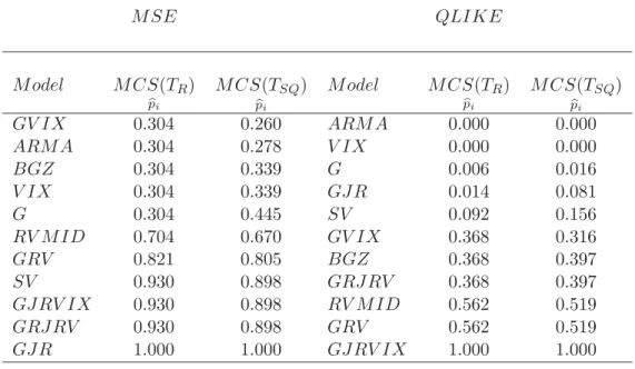
With regard to the shorter forecast horizon over the full sample, as Table 3 shows, the transformed V IX does less well relative to competing MBF but is still included in the MCS. Thep-values for inclusion into the MCS for the full sample period are less than 0.4 under both loss measures and test statistics and is also statistically inseparable from the risk-neutral V IX under MSE. Under the QLIKE loss function, the risk-adjustedV IXforecast is statistically superior to a wide range of models, including the GARCH, EGARCH and SV class of models, as well as the risk-neutralV IX.
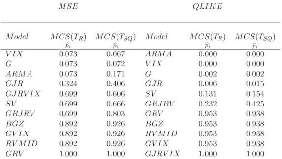
However, over the less volatile shorter sample period, with details provided in Table 4, the transformedV IX is still included in the MCS under both loss measures and test statistics, allp-values are above 0.89. The risk-adjustedV IX
offers significant improvement over the raw V IX forecast, which is excluded from the MCS under both measures and test statistics, it’s highestp-value is
10We generally defer to the results according to QLIKE as Patten and Shephard (2007) has
M SE QLIKE M odel M CS(TR) pi M CS(TSQ) pi M odel M CS(TR) pi M CS(TSQ) pi GV IX 0.110 0.176 GV IX 0.001 0.003 RV M ID 0.110 0.204 ARM A 0.001 0.007 V IX 0.116 0.242 V IX 0.059 0.179 ARM A 0.265 0.303 RV M ID 0.768 0.827 G 0.314 0.343 BGZ 0.768 0.827 BGZ 0.377 0.455 GRJ RV 0.768 0.827 GJ RV IX 0.377 0.455 SV 0.768 0.827 GJ R 0.377 0.455 G 0.776 0.827 SV 0.377 0.517 GRV 0.776 0.827 GRV 0.878 0.878 GJ R 0.776 0.827 GJ RRV 1.000 1.000 GJ RV IX 1.000 1.000 Table 1: MCS of 22-day ahead forecasts for whole sample. The first row rep-resents the first model removed, down to the best performing model in the last row. M SE QLIKE M odel M CS(TR) pi M CS(TSQ) pi M odel M CS(TR) pi M CS(TSQ) pi V IX 0.084 0.027 GV IX 0.000 0.000 G 0.084 0.027 ARM A 0.000 0.000 GV IX 0.084 0.048 V IX 0.032 0.037 GJ R 0.084 0.050 GRJ RV 0.307 0.227 GJ RV IX 0.084 0.065 GJ R 0.394 0.227 ARM A 0.084 0.065 G 0.513 0.290 GRJ RV 0.084 0.081 SV 0.513 0.336 RV M ID 0.305 0.244 RV M ID 0.513 0.451 SV 0.305 0.309 GRV 0.759 0.728 GRV 0.354 0.354 GJ RV IX 0.759 0.746 BGZ 1.000 1.000 BGZ 1.000 1.000 Table 2: MCS of 22-day ahead forecasts for shortened sample.
M SE QLIKE M odel M CS(TR) pi M CS(TSQ) pi M odel M CS(TR) pi M CS(TSQ) pi GV IX 0.304 0.260 ARM A 0.000 0.000 ARM A 0.304 0.278 V IX 0.000 0.000 BGZ 0.304 0.339 G 0.006 0.016 V IX 0.304 0.339 GJ R 0.014 0.081 G 0.304 0.445 SV 0.092 0.156 RV M ID 0.704 0.670 GV IX 0.368 0.316 GRV 0.821 0.805 BGZ 0.368 0.397 SV 0.930 0.898 GRJ RV 0.368 0.397 GJ RV IX 0.930 0.898 RV M ID 0.562 0.519 GRJ RV 0.930 0.898 GRV 0.562 0.519 GJ R 1.000 1.000 GJ RV IX 1.000 1.000 Table 3: MCS of 5-day ahead forecasts for whole sample
0.073 under MSE and the range statistic while hasp-values of zero for both test statistics under QLIKE.
4.3 1 day-ahead forecasts
When examining results for one day-ahead forecasts, as shown in Tables 5 and 6, the transformed V IX is excluded from the MCS under QLIKE and either of the test statistics for both the shortened and full sample; the risk-adjusted
V IX is, however, included in the MCS under the semi-quadratic statistic and MSE loss function for both the shortened and full sample. Unexpectedly, the risk-neutralV IX is included in the MCS for the full sample under MSE and both test statistics.
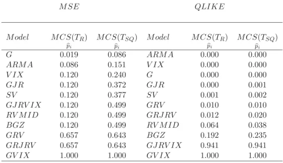
For the shortened sample, the raw V IX again drops out of the MCS un-der both loss functions and test statistics while the transformed V IX is only included in the MCS under MSE using the semi-quadratic statistic. The de-cline in relative forecasting ability of the transformedV IX as the time-horizon shortens is perhaps unsurprising due to the V IX being constructed as a 22-day-ahead forecast which may incorporate information not relevant to shorter forecasting periods. Hence, it seems that while the risk-adjusted V IX yields promising results for the forecast horizon theV IX is constructed for, it is most likely less useful over shorter horizons.
5
Conclusion
Issues relating to forecasting volatility have attracted a great deal of attention in recent years, with such interest undoubtedly piquing given the extreme varia-tions observed in late 2008. As a result, many studies into the relative merits of
M SE QLIKE M odel M CS(TR) pi M CS(TSQ) pi M odel M CS(TR) pi M CS(TSQ) pi V IX 0.073 0.067 ARM A 0.000 0.000 G 0.073 0.072 V IX 0.000 0.000 ARM A 0.073 0.171 G 0.002 0.002 GJ R 0.324 0.406 GJ R 0.006 0.015 GJ RV IX 0.699 0.606 SV 0.131 0.154 SV 0.699 0.666 GRJ RV 0.232 0.425 GRJ RV 0.699 0.803 GRV 0.953 0.938 BGZ 0.892 0.926 BGZ 0.953 0.938 GV IX 0.892 0.926 RV M ID 0.953 0.938 RV M ID 0.892 0.926 GV IX 0.953 0.938 GRV 1.000 1.000 GJ RV IX 1.000 1.000 Table 4: MCS of 5-day ahead forecasts for shortened sample
M SE QLIKE M odel M CS(TR) pi M CS(TSQ) pi M odel M CS(TR) pi M CS(TSQ) pi BGZ 0.121 0.378 ARM A 0.000 0.000 G 0.139 0.428 V IX 0.000 0.000 GV IX 0.415 0.733 G 0.000 0.000 GJ RV IX 0.421 0.765 SV 0.000 0.001 GJ R 0.421 0.765 GJ R 0.000 0.007 SV 0.689 0.871 GRV 0.016 0.049 RV M ID 0.689 0.871 BGZ 0.051 0.074 ARM A 0.689 0.871 RV M ID 0.051 0.074 GRJ RV 0.942 0.934 GRJ RV 0.051 0.074 GRV 0.942 0.934 GV IX 0.224 0.224 V IX 1.000 1.000 GJ RV IX 1.000 1.000 Table 5: MCS of 1-day ahead forecasts for whole sample
M SE QLIKE M odel M CS(TR) pi M CS(TSQ) pi M odel M CS(TR) pi M CS(TSQ) pi G 0.019 0.086 ARM A 0.000 0.000 ARM A 0.086 0.151 V IX 0.000 0.000 V IX 0.120 0.240 G 0.000 0.000 GJ R 0.120 0.372 GJ R 0.000 0.001 SV 0.120 0.377 SV 0.001 0.002 GJ RV IX 0.120 0.499 GRV 0.010 0.010 RV M ID 0.120 0.499 GRJ RV 0.012 0.020 BGZ 0.120 0.499 RV M ID 0.064 0.038 GRV 0.657 0.643 BGZ 0.192 0.235 GRJ RV 0.657 0.643 GJ RV IX 0.941 0.941 GV IX 1.000 1.000 GV IX 1.000 1.000 Table 6: MCS of 1-day ahead forecasts for shortened sample
implied and model based volatility forecasts have been conducted, and although it has often been found that implied volatility offers superior performance, many studies disagreed. Recently, Becker & Clements (2008) showed that the V IX
was statistically inferior to a combination of model based forecasts, inferring that the V IX does not represent an optimal combination of volatility fore-casts. However, it was argued in this paper that these comparisons may not have been “fair” given that they have involved comparisons of risk-neutral im-plied volatility forecasts while model based forecasts are generated under the physical measure. Using the methodology of Bollerslev, Gibson & Zhou (2008), a transformedV IX forecast that incorporated the volatility risk-premium was generated and its forecast performance compared with model based forecasts of S&P 500 Index volatility via the model confidence set technology of Hansen
et al. (2003a, 2003b)
The transformedV IX offered significant improvement in forecasting ability over the risk-neutral V IX in four of the six samples considered. When com-pared under the QLIKE loss function with model based forecasts of 22-day-ahead volatility, the risk-adjusted V IX was included in the model confidence set over both the shortened and full-length sample periods, implying it performs at least as well as model based forecasts. We put forth that this is a significant addition to the volatility forecasting literature relating to implied volatility.
Overall, this paper shows that if one correctly accounts for the volatility risk-premium, the market determined forecast of volatility over a 22-day horizon is in fact of equal predictive accuracy to a small number of model based forecasts. This result clarifies confusion from many prior studies which have, for the most part, typically conducted pair-wise comparisons and have neglected adjusting for the volatility risk-premium.
References
Andersen, T.G., Bollerslev, T., Diebold, F.X. & Labys, P. (1999). (Under-standing, optimizing, using and forecasting) Realized Volatility and Correla-tion. Working Paper, University of Pennsylvania.
Andersen T.G., Bollerslev T., Diebold F.X. & Labys P. (2001). The distribu-tion of exchange rate volatility. Journal of the American Statistical Associa-tion 96, 42-55.
Andersen T.G., Bollerslev T., Diebold F.X. & Labys P. (2003). Modeling and forecasting realized volatility.Econometrica. 71, 579-625.
Andersen T.G., Bollerslev T. & N. Meddahi. (2004). Analytical Evaluation of Volatility Forecasts.International Economic Review, 45, 1079-1110.
Andersen T.G., Bollerslev T. & N. Meddahi. (2005). Correcting the Er-rors: Volatility Forecast Evaluation Using High-Frequency Data and Realized Volatilities. Econometrica 73, 279-296.
Barndorff-Nielson, O. & Shephard, N. (2004). A Feasible Central Limit Theory for Realised Volatility under Leverage.Manuscript, Nuffield College, Oxford University.
Becker, R., & Clements, A. (2008). Are combination forecasts of S&P 500 volatility statistically superior?International Journal of Forecasting., 24, 122-133.
Becker, R., Clements, A. & White, S. (2006). Does implied volatility provide any information beyond that captured in model-based volatility forecasts?, forthcoming inJournal of Banking and Finance.
Blair B.J., Poon S-H. & Taylor S.J. (2001). Forecasting S&P 100 volatility: the incremental information content of implied volatilities and high-frequency index returns.Journal of Econometrics, 105, 5-26.
Bollerslev, T., (1986). Generalized Autoregressive Conditional Heteroskedas-ticity. Journal of Econometrics., 31, 307-27
Bollerslev, T., Gibson, M., & Zhou, H. (2008). Dynamic Estimation of Volatil-ity Risk Premia and Investor Risk Aversion from Option-Implied and Realized Volatilities. unpublished manuscript, Duke University.
Bollerslev, T., & Zho, H. (2002). Estimating Stochastic Volatility Diffusion Using Conditional Moments of Integrated Volatility.Journal of Econometrics, 109, 3365.
Britten-Jones, M., & Neuberger, A. (2000) Option Prices, Implied Price Pro-cesses, and Stochastic Volatility. Journal of Finance, 55, 839866.
Canina, L. & Figlewski, S. (1993). The information content of implied volatil-ity.Review of Financial Studies, 6, 659-681.
Campbell, J.Y., Lo, A.W. & MacKinlay, A.G. (1997). The Econometrics of Financial Markets, Princeton University Press, Princeton NJ.
Chicago Board of Options Exchange (2003) VIX, CBOE Volatility Index. Christensen B.J. & Prabhala N.R. (1998). The relation between implied and realized volatility. Journal of Financial Economics, 50, 125-150.
Clements, A.E., Hurn, A.S. & White, S.I. (2003). Discretised Non-Linear Filtering of Dynamic Latent Variable Models with Application to Stochastic Volatility, Discussion Paper No 179, School of Economics and Finance, Queens-land University of Technology.
Cochrane, J.H. (2001).Asset Pricing, Princeton University Press: Princeton, NJ.
Day, T.E. & Lewis, C.M. (1992). Stock market volatility and the information content of stock index options.Journal of Econometrics, 52, 267-287.
Ederington, L.H. & Guan, W. (2002). Is implied volatility an informationally efficient and effective predictor of future volatility?, Journal of Risk, 4, 3. Engle, R.F & Ng, V.K. (1991). Measuring and testing the impact of news on volatility, Journal of Finance, 48, 1749-1778.
Fleming J. (1998). The quality of market volatility forecasts implied by S&P 100 index option prices,Journal of Empirical Finance,5, 317-345.
Fleming, J., Ostdiek, B. & Whaely, R.E. (1995). Predicting stock market volatility: a new measure,Journal of Futures Markets, 15, 265-302.
Glosten, L.R., Jagannathan, R and.Runkle, D.E. (1993). On the relation be-tween the expected value and the volatility of the nominal excess return on stocks.Journal of Finance, 48, 1779-1801.
Gourieroux C. & Jasiak J. (2001).Financial Econometrics. Princeton Univer-sity Press: Princeton NJ.
Hansen, P.R., Lunde, A. & Nason, J.M. (2003). Choosing the best volatility models: the model confidence set appraoch,Oxford Bulletin of Economics and Statistics 65, 839-861.
Hansen, P.R., Lunde, A. & Nason, J.M. (2003). Model confidence sets for forecasting models approach, Working Paper 2003-5, Brown University. Heston, S. (1993). A Closed-Form Solution for Options with Stochastic Volatil-ity with Applications to Bond and Currency Options. Review of Financial Studies, 6, 327343.
Jiang, G., & Yisong, T. (2005). Model-Free Implied Volatility and Its Infor-mation Content.Review of Financial Studies, 18, 13051342.
Jorion P. (1995). Predicting volatility in the foreign exchange market.Journal of Finance,50, 507-528.
Koopman, S.J. and Jungbacker, B. & Hol, E. (2005). Forecasting daily variabil-ity of the S&P 100 stock index using historical, realised and implied volatilvariabil-ity measurements.Journal of Empirical Finance, 12, 445-475.
Lahiri, S.N. (1999) Theoretical comparison of block bootstrap methods, An-nals of Statistics, 27, 386-404.
Lameroureux, C.G. & Lastrapes, W. (1993). Forecasting stock-return variance: toward an understanding of stochastic implied volatilities,Review of Financial Studies, 6, 293-326.
Meddahi, N. (2002). Theoretical Comparison Between Integrated and Realized Volatility. Journal of Applied Econometrics, 17, 479-508.
Mincer, J. and Zarnowitz, V. (1969). The Evaluation of Economic Forecasts, In: Zarnowitz, J. (Ed.) Economic Forecasts and Expectations, National Bu-reau of Economic Research, New York.
Newey, W. K., & West, K. D. (1987). A Simple Positive Semi-Definite Het-eroskedasticity and Autocorrelation Consistent Covariance Matrix. Economet-rica, 55, 703-708.
Pantula, S.G. (1989). Testing for unit roots in time series data, Econometric Theory, 5, 256-271.
Patton, A.J. (2005). Volatility forecast comparison using imperfect volatility proxies. Unpublised Manuscript.
Patton, A. and Sheppard, K. (2007). Evaluating Volatility Forecasts, in Hand-book of Financial Time Series, Andersen, T.G., Davis, R.A., Kreiss, J.P. and Mikosch, T. eds., Springer-Verlag.
Politis, D.N. & J.P. Romano (1994) The Stationary Bootstrap.Journal of the American Statistical Association, 89, 1303-1313.
Poon S-H. & Granger C.W.J. (2003). Forecasting volatility in financial mar-kets: a review. Journal of Economic Literature,41, 478-539.
Poon S-H. & Granger C.W.J. (2005). Practical Issues in forecasting volatility.
Financial Analysts Journal, 61, 45-56.
Taylor, S. J. (2005).Asset Price Dynamics, Volatility, and Prediction. Prince-ton University Press: PrincePrince-ton NJ.
White, H. (2000). A Reality Check For Data Snooping. Econometrica, 68, 1097-1127.
List
of
NCER
Working
Papers
No. 44 (Download full text)
Adam Clements and Annastiina Silvennoinen
On the economic benefit of utility based estimation of a volatility model
No. 43 (Download full text)
Adam Clements and Ralf Becker
A nonparametric approach to forecasting realized volatility
No. 42 (Download full text)
Uwe Dulleck, Rudolf Kerschbamer and Matthias Sutter
The Economics of Credence Goods: On the Role of Liability, Verifiability, Reputation and Competition
No. 41 (Download full text)
Adam Clements, Mark Doolan, Stan Hurn and Ralf Becker
On the efficacy of techniques for evaluating multivariate volatility forecasts
No. 40 (Download full text)
Lawrence M. Kahn
The Economics of Discrimination: Evidence from Basketball
No. 39 (Download full text)
Don Harding and Adrian Pagan
An Econometric Analysis of Some Models for Constructed Binary Time Series
No. 38 (Download full text)
Richard Dennis
Timeless Perspective Policymaking: When is Discretion Superior?
No. 37 (Download full text)
Paul Frijters, Amy Y.C. Liu and Xin Meng
Are optimistic expectations keeping the Chinese happy?
No. 36 (Download full text)
Benno Torgler, Markus Schaffner, Bruno S. Frey, Sascha L. Schmidt and Uwe Dulleck
Inequality Aversion and Performance in and on the Field
No. 35 (Download full text)
T M Christensen, A. S. Hurn and K A Lindsay
Discrete time‐series models when counts are unobservable
No. 34 (Download full text)
Adam Clements, A S Hurn and K A Lindsay
Developing analytical distributions for temperature indices for the purposes of pricing temperature‐based weather derivatives
No. 33 (Download full text)
Adam Clements, A S Hurn and K A Lindsay
No. 32 (Download full text)
T M Christensen, A S Hurn and K A Lindsay
The Devil is in the Detail: Hints for Practical Optimisation
No. 31 (Download full text)
Uwe Dulleck, Franz Hackl, Bernhard Weiss and Rudolf Winter‐Ebmer
Buying Online: Sequential Decision Making by Shopbot Visitors
No. 30 (Download full text)
Richard Dennis
Model Uncertainty and Monetary Policy
No. 29 (Download full text)
Richard Dennis
The Frequency of Price Adjustment and New Keynesian Business Cycle Dynamics
No. 28 (Download full text)
Paul Frijters and Aydogan Ulker
Robustness in Health Research: Do differences in health measures, techniques, and time frame matter?
No. 27 (Download full text)
Paul Frijters, David W. Johnston, Manisha Shah and Michael A. Shields
Early Child Development and Maternal Labor Force Participation: Using Handedness as an Instrument
No. 26 (Download full text)
Paul Frijters and Tony Beatton
The mystery of the U‐shaped relationship between happiness and age.
No. 25 (Download full text)
T M Christensen, A S Hurn and K A Lindsay
It never rains but it pours: Modelling the persistence of spikes in electricity prices
No. 24 (Download full text)
Ralf Becker, Adam Clements and Andrew McClelland
The Jump component of S&P 500 volatility and the VIX index
No. 23 (Download full text)
A. S. Hurn and V.Pavlov
Momentum in Australian Stock Returns: An Update
No. 22 (Download full text)
Mardi Dungey, George Milunovich and Susan Thorp
Unobservable Shocks as Carriers of Contagion: A Dynamic Analysis Using Identified Structural GARCH
No. 21 (Download full text) (forthcoming)
Mardi Dungey and Adrian Pagan
No. 20 (Download full text)
Benno Torgler, Nemanja Antic and Uwe Dulleck
Mirror, Mirror on the Wall, who is the Happiest of Them All?
No. 19 (Download full text)
Justina AV Fischer and Benno Torgler
Social Capital And Relative Income Concerns: Evidence From 26 Countries
No. 18 (Download full text)
Ralf Becker and Adam Clements
Forecasting stock market volatility conditional on macroeconomic conditions.
No. 17 (Download full text)
Ralf Becker and Adam Clements
Are combination forecasts of S&P 500 volatility statistically superior?
No. 16 (Download full text)
Uwe Dulleck and Neil Foster
Imported Equipment, Human Capital and Economic Growth in Developing Countries
No. 15 (Download full text)
Ralf Becker, Adam Clements and James Curchin
Does implied volatility reflect a wider information set than econometric forecasts?
No. 14 (Download full text)
Renee Fry and Adrian Pagan
Some Issues in Using Sign Restrictions for Identifying Structural VARs
No. 13 (Download full text)
Adrian Pagan
Weak Instruments: A Guide to the Literature
No. 12 (Download full text)
Ronald G. Cummings, Jorge Martinez‐Vazquez, Michael McKee and Benno Torgler
Effects of Tax Morale on Tax Compliance: Experimental and Survey Evidence
No. 11 (Download full text)
Benno Torgler, Sascha L. Schmidt and Bruno S. Frey
The Power of Positional Concerns: A Panel Analysis
No. 10 (Download full text)
Ralf Becker, Stan Hurn and Vlad Pavlov
Modelling Spikes in Electricity Prices
No. 9 (Download full text)
A. Hurn, J. Jeisman and K. Lindsay
Teaching an Old Dog New Tricks: Improved Estimation of the Parameters of Stochastic Differential Equations by Numerical Solution of the Fokker‐Planck Equation
No. 8 (Download full text)
Stan Hurn and Ralf Becker
Testing for nonlinearity in mean in the presence of heteroskedasticity.
No. 7 (Download full text) (published)
Adrian Pagan and Hashem Pesaran
On Econometric Analysis of Structural Systems with Permanent and Transitory Shocks and Exogenous Variables.
No. 6 (Download full text) (published)
Martin Fukac and Adrian Pagan
Limited Information Estimation and Evaluation of DSGE Models.
No. 5 (Download full text)
Andrew E. Clark, Paul Frijters and Michael A. Shields
Income and Happiness: Evidence, Explanations and Economic Implications.
No. 4 (Download full text)
Louis J. Maccini and Adrian Pagan
Inventories, Fluctuations and Business Cycles.
No. 3 (Download full text)
Adam Clements, Stan Hurn and Scott White
Estimating Stochastic Volatility Models Using a Discrete Non‐linear Filter.
No. 2 (Download full text)
Stan Hurn, J.Jeisman and K.A. Lindsay
Seeing the Wood for the Trees: A Critical Evaluation of Methods to Estimate the Parameters of Stochastic Differential Equations.
No. 1 (Download full text)
Adrian Pagan and Don Harding
The Econometric Analysis of Constructed Binary Time Series.