UCLA
UCLA Electronic Theses and Dissertations
Title
Three Essays on Unobserved Heterogeneity in Panel and Network Data Models
Permalink https://escholarship.org/uc/item/9x23540z Author Shang, Hualei Publication Date 2020 Peer reviewed|Thesis/dissertation
eScholarship.org Powered by the California Digital Library
UNIVERSITY OF CALIFORNIA Los Angeles
Three Essays on Unobserved Heterogeneity in Panel and Network Data Models
A dissertation submitted in partial satisfaction of the requirements for the degree Doctor of Philosophy
in Economics
by
Hualei Shang
c
Copyright by Hualei Shang
ABSTRACT OF THE DISSERTATION
Three Essays on Unobserved Heterogeneity in Panel and Network Data Models
by
Hualei Shang
Doctor of Philosophy in Economics University of California, Los Angeles, 2020
Professor Rosa Liliana Matzkin, Chair
This dissertation consists of three chapters that study unobserved heterogeneity in panel and network data models. In Chapter 1, I propose a semi-nonparametric panel data model with a latent group structure. I assume that individual parameters are heterogeneous across groups but homogeneous within a group while the group membership is unknown. I first approximate the infinite-dimensional function with a sieve expansion; then, I propose a Classifier-Lasso(C-Lasso) procedure to simultaneously identify the individuals’ membership and estimate the group-specific parameters. I show that: (i) the classification exhibits uniform consistency; (ii) C-Lasso and post-Lasso estimators achieve oracle properties so that they are asymptotically equivalent to infeasible estimators as if the group membership is known; and (iii) the estimators are consistent and asymptotically normally distributed. Simulations demonstrate an excellent finite sample performance of this approach in both classification and estimation.
In Chapter 2 (joint with Wenyu Zhou), we study a nonparametric additive panel regres-sion model with grouped heterogeneity. The model can be regarded as a natural extenregres-sion to the heterogeneous panel model studied in Su, Shi, and Phillips (2016). We propose to estimate the nonparametric components using a sieve-approximation-based Classifier-Lasso
method. We establish the asymptotic properties of the estimator and show that they enjoy the so-called oracle property. In addition, we present the decision rule for group classifica-tion and establish its consistency. Then, a BIC-type informaclassifica-tion criterion is developed to determine the group pattern of each nonparametric component. We further investigate the finite sample performance of the estimation method and the information criterion through Monte Carlo simulations. Results show that both work well. Finally, we apply the model and the estimation method to study the demand for cigarettes in the United States using panel data of 46 states from 1963 to 1992.
In Chapter 3, I study a network sample selection model in which 1) bilateral fixed effects enter the pairwise outcome equation additively; 2) link formation depends on latent variables from both sides nonparametrically. I first propose a four-cycle structure to difference out the fixed effects; next, utilizing the idea proposed in Auerbach (2019), I manage to use the kernel function to control for the selection bias. I then introduce estimators for the parameters of interest and characterize their asymptotic properties.
The dissertation of Hualei Shang is approved.
Ying Nian Wu
Denis Nikolaye Chetverikov Shuyang Sheng
Zhipeng Liao
Rosa Liliana Matzkin, Committee Chair
University of California, Los Angeles 2020
DEDICATIONS
To my parents and lovely niece
Contents
1 Semi-Nonparametric Panel Data Models with Latent Structures 1
1.1 Introduction . . . 2
1.2 Penalized Sieve Estimation . . . 7
1.2.1 Semi-Nonparametric Panel Data Structure Models . . . 7
1.2.2 Sieve Approximation . . . 8
1.2.3 Penalized Estimation of α and f . . . 10
1.3 Asymptotic Properties . . . 11
1.3.1 Assumptions . . . 11
1.3.2 Preliminary Rates of Convergence . . . 17
1.3.3 Classification Consistency . . . 18
1.3.4 The Oracle Property and Asymptotic Distributions . . . 19
1.3.5 Determination of Number of Groups . . . 22
1.4 Simulation . . . 24
1.4.1 Data Generating Process . . . 24
1.4.2 Main Result . . . 25
1.4.3 Comparison with Complete Homogeneity and Heterogeneity . . . 29
1.4.4 Comparison with Misspecified Parametric model . . . 31
1.5 Conclusion . . . 33
1.A Proofs of the Main Results . . . 34
2 Nonparametric Additive Panel Regression Models with Grouped Hetero-geneity 64 2.1 Introduction . . . 65 2.2 Model . . . 68 2.3 Estimation . . . 69 2.3.1 Sieve Approximation . . . 70
2.3.2 Penalized Estimation of h and f . . . 71
2.4 Asymptotic Properties . . . 73
2.4.1 Preliminary Rates of Convergence . . . 73
2.4.2 Classification Consistency . . . 78
2.4.3 The Oracle Property and Asymptotic Distributions . . . 79
2.4.4 Determination of Number of Groups . . . 81
2.5 Simulation . . . 83
2.5.1 Data Generating Process . . . 83
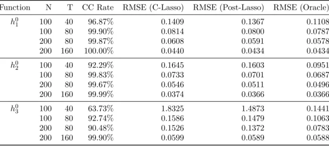
2.5.2 Simulation Results . . . 86
2.6 Empirical Illustration . . . 88
2.7 Conclusion . . . 92
2.A Proofs of the Main Results . . . 93
2.B Proofs of Technical Lemmas . . . 104
3 A Network Sample Selection Model 114 3.1 Motivation . . . 115
3.2 Model Setup . . . 118
3.2.1 Explanation of the Link Formation Process . . . 119
3.3 Estimation Strategy . . . 121
3.4 Asymptotic Properties . . . 125
3.4.1 Consistency . . . 125
3.4.2 Asymptotic Distribution when ωi has Finite Support . . . 127
3.4.3 Asymptotic Distribution when ωi is Continuous . . . 128
3.5 Extension to Directed Networks . . . 129 3.6 Conclusion . . . 132
List of Figures
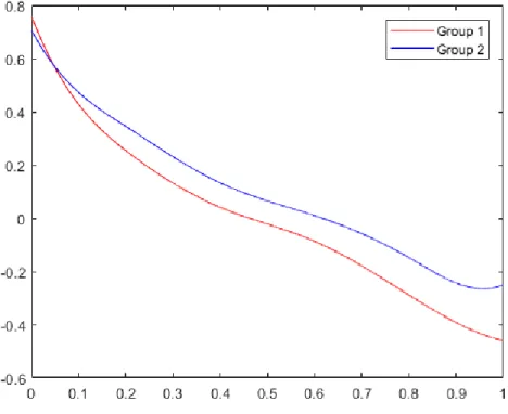
2.1 Estimated Functions ofh1 . . . 90
2.2 Estimated Functions ofh2 . . . 91
3.1 Trade Flows . . . 117
3.2 Trade with Same Countries . . . 120
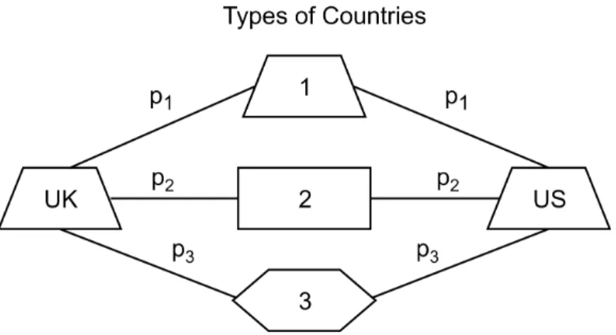
3.3 Trade with Same Countries with Same Probabilities . . . 120
3.4 Countries of the Same Type . . . 120
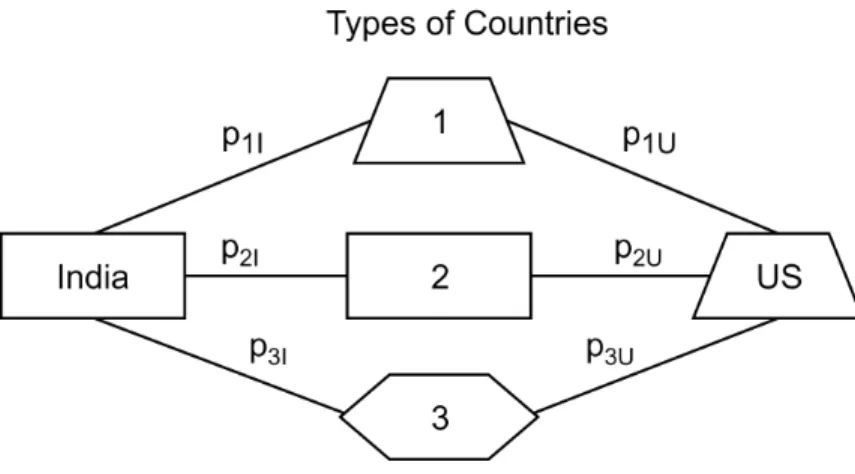
3.5 Countries of Different Types . . . 121
3.6 Four Cycle . . . 122
3.7 Directed Four Cycle . . . 131
List of Tables
1.1 Literature Review on Classification . . . 6
1.2 RMSE (Maximum) of C-Lasso and post-Lasso Estimators in DGP 1 . . . 27
1.3 RMSE of C-Lasso and post-Lasso Estimators in DGP 1 . . . 28
1.4 Comparison with Complete Homogeneity and Heterogeneity in DGP 1 . . . 30
1.5 Comparison with Misspecified Parametric Model in DGP 1 . . . 31
1.6 Comparison with Misspecified Parametric Model in DGP 2 . . . 32
2.1 Simulation Results for Group-specific Parameters in DGP 1 . . . 87
2.2 Simulation Results for Group-specific Parameters in DGP 2 . . . 87
ACKNOWLEDGMENT
I am grateful to Rosa Matzkin, Zhipeng Liao, Shuyang Sheng, Denis Chetverikov, and Ying Nian Wu for invaluable guidance and continuous support. I thank Jinyong Hahn, Andres Santos, and participants at UCLA econometrics proseminars for helpful comments and dis-cussions. All errors, of course, are mine.
VITA
Education
University of California, Los Angeles Los Angeles, USA C.Phil., Economics, Department of Economics 2016 M.A., Economics, Department of Economics 2015 Peking University Beijing, China M.A., Economics, National School of Development 2014 Tsinghua University Beijing, China B.E., Engineering Physics, Department of Engineering Physics 2008
Fellowships and Awards
UCLA Dissertation Year Fellowship, 2019-2020
UCLA Economic Departmental Teaching Assistantship, 2015-2019 UCLA Economic Departmental Fellowship, 2014-2015
Graduate Dean’s Scholar Award, UCLA, 2014-2015
Best Teaching Assistant Award, Peking University, 2011-2012
Teaching Experience Instructor
Microeconomic Theory I, UCLA, Summer 2018 Teaching Assistant
Econometrics Laboratory, UCLA, Summer 2019, Spring 2017 Microeconomic Theory I, UCLA, Spring 2018, Spring 2016
Statistics for Economists, UCLA, Winter 2018, Fall 2018, Winter 2017 Microeconomic Theory II, UCLA, Fall 2016
Principles of Economics II, UCLA, Winter 2016 Principles of Economics I, UCLA, Fall 2015
Intermediate Macroeconomics, Peking University, Fall 2013, Spring 2012 Advanced Econometrics (Masters), Peking University, Fall 2012
Intermediate Econometrics, Peking University, Fall 2012
Chapter 1
Semi-Nonparametric Panel Data
Models with Latent Structures
1.1
Introduction
In semi-nonparametric panel data models, it is almost universal to assume that the regression parameters are the same across individuals, while unobserved heterogeneity is merely mod-eled through individual-specific effects. However, since most panel data cover cross-sectional units with different characteristics, to control for individual heterogeneity remains a chal-lenge. One important task is how to model the influence of heterogeneity on the individual regression parameters. To tackle the problem while preserving the power of cross-sectional averaging, I propose a semi-nonparametric panel data model with a latent group structure. I assume that individuals belong to different groups while the group identity is unknown a priori. Individual regression parameters are the same within the group but differ across groups. In Economics, the groups could be understood as different convergence clubs in the economic growth studies (Phillips and Sul (2007)), stock returns in different sectors in financial markets (Ke, Fan, and Wu (2015)), spatial geographic groupings in economic geography (Bester and Hansen (2016); Fan, Lv, and Qi (2011)) or multiplicity of Nash equilibria in game theory or Macroeconomics models (Hahn and Moon (2010)). Several important examples and policy implications will be discussed at the end of this section.
This group structure modeling reaches a good balance between its two alternatives: com-plete parameter homogeneity or comcom-plete parameter heterogeneity. Traditional panel data models always assume that individuals share the same parameters. Although this approach is easy to implement and achieves good convergence rate, homogeneity assumption has been frequently rejected in empirical studies; see Hsiao and Tahmiscioglu (1997), Lee, Pesaran, and Smith (1997), Durlauf, Kourtellos, and Minkin (2001), Phillips and Sul (2007), Brown-ing and Carro (2007), BrownBrown-ing and Carro (2010), Su and Chen (2013) and BrownBrown-ing and Carro (2014). To the other extreme, if we allow for complete parameter heterogeneity, the key advantage of working with panel data is lost. If the time dimension is short, estimation could be very imprecise. See survey papers by Baltagi, Bresson, and Pirotte (2008) and Hsiao and Pesaran (2008). Compared with the two pieces of literature above, the group
structure approach simultaneously alleviates the misspecification problem common in the first one and preserves the power of cross-section averaging lost in the second one.
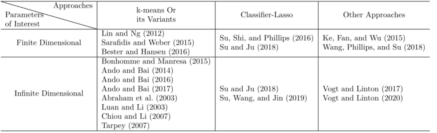
In the literature of panel structure modeling, there are two dimensions to consider. First, whether the parameters of interest are finite or infinite-dimensional; Second, what approach to use. Please see Table 1.1 for a summary. I discuss the literature mainly according to the approaches they implement but will also mention the parameters of interest in the process. First, the k-means algorithm or its variants are commonly used to classify individuals into different groups. Lin and Ng (2012) and Sarafidis and Weber (2015) studied linear panel data models with finite dimensional coefficients following some group structure. Bonhomme and Manresa (2015) focuses on the grouped patterns of time-varying fixed effects. Ando and Bai (2014), Ando and Bai (2016) and Ando and Bai (2017) generalized Bonhomme and Manresa (2015) and studied panel data models where interactive fixed effects exhibit some group structure. Abraham et al. (2003), Luan and Li (2003), Chiou and Li (2007) and Tarpey (2007) applied the k-means algorithm or its variants to different realizations of random curves that depend on a deterministic index t∈ T.
Another approach, called classifier-Lasso (C-lasso), proposed by Su, Shi, and Phillips (2016), treated clustering as a process of shrinking individual-specific coefficients into some group-specific parameters. They imposed the group structure on finite dimensional parame-ters. Su and Ju (2018) extended this method to include interactive fixed effects. Su, Wang, and Jin (2019) assumed that time-varying coefficients follow some group structures.
There also exist some other classifying methods. Ke, Fan, and Wu (2015) proposed a clustering algorithm in regression via data-driven segmentation (CARDS). Wang, Phillips, and Su (2018) further generalized it into the panel data. Vogt and Linton (2017) implemented a thresholding method combining with kernel estimation to classify nonparametric functions into different groups. Vogt and Linton (2020) further developed a clustering method that does not rely on any smooth parameters, like the bandwidth or number of basis functions.
semi-nonparametric panel data models instead. C-lasso enjoys several significant advantages over the k-means algorithm and other alternatives. First, it allows some individuals left unclassified, adding more flexibility to the model. Second, the k-means method relies heavily on the initial values of the group identity, while C-Lasso is not sensitive to that. Third, the computation burden of k-means is more significant than that of C-lasso. Finally, C-lasso could be easily combined with some other methods.
Practically, my method could be separated into two steps. I first approximate the infinite-dimensional functions with a sieve expansion and then use C-Lasso to shrink individual-specific coefficients of basis functions into some group-individual-specific parameters.
The main contribution of this paper is that I generalize the latent group structures from parametric to semi-nonparametric panel data models. Thus, further exploration beyond the parametric specification of the unobserved heterogeneity in response mechanisms becomes possible. Although Su, Wang, and Jin (2019), Vogt and Linton (2017) and Vogt and Linton (2020) also considered clustering of functions, in Su, Wang, and Jin (2019), the regressor is one-dimensional deterministic (t/T) while in my paper, they could be multiple-dimensional general random variables. The approaches in Vogt and Linton (2017) and Vogt and Linton (2020) are difficult to be applied to partially linear models; however, in my research, partially linear and nonparametric models are of no significant difference. So far as I know, my paper is the first one in the literature to impose group structures to semi-nonparametric panel data models flexibly.
I also contribute to the extensive literature of estimation in semi-nonparametric panel data models, including, but not limited to, partially linear and nonparametric panel data models. In addition to the estimation, my approach simultaneously identifies individuals’ membership. However, this doesn’t affect the asymptotic properties of the estimators, which are equivalent to those of the oracle estimators that use individual group identity information. The latter are well studied in the literature. For detailed discussions, I direct readers to survey papers by Su and Ullah (2011), Ai and Li (2008) and Ullah and Roy (1998).
To further illustrate applications of my method, I discuss the following three examples:
Example 1 (Learning Curve): In Atkin, Khandelwal, and Osman (2017), the authors
conducted a random experiment for rug producers in Egypt. They generated exogenous vari-ation in access to foreign markets and studied the impact of exporting on firm performance. The most crucial step is to estimate how the quality changes as the volume of production increases, i.e., the learning curves. They assumed that different firms share the same learning curve.
However, due to unobserved heterogeneity (for example, the management levels of owners or proficiencies of workers in different firms might differ.), it might not be appropriate to make such a homogeneity assumption. My approach then would complement their study to further explore the heterogeneity of different firms in terms of learning.
Example 2 (Trade Cost): Atkin and Donaldson (2015) used newly collected CPI
microdata from Ethiopia and Nigeria to study how cost-shifting characteristics (such as distance) affect the spatial price gaps.
However, distance is only an imperfect proxy for measuring transportation costs. The origin-destination paths exhibit considerable unobserved heterogeneity (for example, the quality of the roads is unobserved.). Although the authors also tried the quickest-route travel time measure as a more plausible alternative for the geographic distance, the same concern remains.
My method, on the other hand, would help to capture the heterogeneity of routes by merely imposing a group structure (high quality and low quality roads) on the effect of distance on price gaps.
Example 3 (Policy Analysis): Clemens, Lewis, and Postel (2018) evaluated the labor
market effects of abrogation of the manual laborer (Bracero) agreements between the United States and Mexico. They estimated how the exclusion of Mexican farmworkers affect the employment and wages of domestic workers.
To study the heterogeneity of the effects, they split the states of the US into three groups using Bracero fraction (B/L, the ratio of Bracero workers and the whole labor force) as a criterion: no exposure with B/L= 0, low exposure with 0< B/L < 0.2 and high exposure with B/L >0.2.
Even though this criterion might capture some heterogeneity of the influence of the policy on different states, it would be useful to use my approach at least as a robustness check. I could automatically accomplish the classification and estimation with an additional harmless assumption that the effect could be expressed as a time-varying function. The advantage, however, is to avoid any subjective judgment which might be arbitrary.
Table 1.1: Literature Review on Classification
Parameters of Interest
Approaches
k-means Or
its Variants Classifier-Lasso Other Approaches
Finite Dimensional
Lin and Ng (2012) Sarafidis and Weber (2015) Bester and Hansen (2016)
Su, Shi, and Phillips (2016) Su and Ju (2018)
Ke, Fan, and Wu (2015) Wang, Phillips, and Su (2018)
Infinite Dimensional
Bonhomme and Manresa (2015) Ando and Bai (2014)
Ando and Bai (2016) Ando and Bai (2017) Abraham et al. (2003) Luan and Li (2003) Chiou and Li (2007) Tarpey (2007)
Su and Ju (2018) Su, Wang, and Jin (2019)
Vogt and Linton (2017) Vogt and Linton (2020)
The rest of the paper is organized as follows. Section 1.2 discusses the model. Section 1.3 presents the estimation and inference results. Section 1.4 reports Monto Carlo simulation findings. Section 1.5 concludes. All proofs of the main results are given in the Appendix.
Notation: Throughout the paper, I consider the case that (N, T) pass jointly to infinity,
which is denoted as (N, T) → ∞. For any real value matrix A, I write the transpose A0, the Frobenius normkAkF ≡ tr(AA0)12
and the Moore-Penrose inverse A−. When A is symmetric, I denoteµmax(A) andµmin(A) as its largest and lowest eigenvalues, respectively.
For a square integrable function f defined on the support Ω, kfk2 denotes its L2 norm:
kfk2 ≡nR Ω f(x) 2 dxo 1 2
. The operator →P means convergence in probability, →D convergence in distribution. α β denotes thatα and β are of the same magnitude, i.e., α =O(β) and
β =O(α). I use superscript 0 to denote the true values of parameters.
1.2
Penalized Sieve Estimation
In this section, I assume that the number of groups K0 is known and will discuss in Section
1.3.5 how to determine it.
1.2.1
Semi-Nonparametric Panel Data Structure Models
I mainly focus on the partially linear model, since 1) all the results hold for nonparametric models as long as the conditions of finite-dimensional parameters are excluded. 2) it is more involving to develop the theory for partially linear models. I will briefly mention how to apply the method into nonparametric models when necessary.
A partially linear model in panel data takes the following form:
yit=µi+ωit0 βi+hi(xit) +uit uit =σi(ωit, xit)εit (1.1)
where i = 1,2, ..., N, t = 1,2, ..., T. ωit is a p×1 vector of regressors. xit is a d×1 vector
of controls that affect the outcome throughhi(xit). µi’s represent the unobserved individual
fixed effects which might be correlated with ωit and xit. εit has mean 0 and variance 1 and
is independent of {ωit, xit}, so uit is the error term with mean 0 and variance σ2i(ωit, xit)
conditional on {ωit, xit}.
I denote the true value of βi as βi0, and hi(xit) as h0i(xit) with a compact support X.
I assume that the finite-dimensional parameters βi’s and infinite-dimensional functions hi’s
exhibit the following group pattern
βi0 = K0 X k=1 α0k1{i∈G0k} (1.2) h0i(xit) = K0 X k=1 fk0(xit)1{i∈G0k} for any xit∈ X (1.3)
which means that individuals within groupkshare the same parameterα0
kand same
func-tion f0
k. {G0k, k = 1,2, ...K0} are mutually exclusive, meaning that ∪K
0
k=1G0k ={1,2, ..., N},
and G0
k ∩ G0j = ∅ if j 6= k. Nk = #G0k denotes the cardinality of G0k, and obviously
PK0
k=1Nk=N. The notations I use are consistent with Su, Shi, and Phillips (2016).
Following Sun (2005), Lin and Ng (2012), Bonhomme and Manresa (2015) and Su, Shi, and Phillips (2016), I assume that individual group identity doesn’t change over time. Let
α = (α1, ..., αK0) 0
, f = (f1, ..., fK0) 0
and denote the corresponding true values as α0 and f0, respectively.
The goal is to determine individuals’ group identities and to estimate the group-specific parameters α and f.
Remark. For nonparametric panel data models, equation 1.1 becomes
yit =µi+hi(xit) +uit uit=σi(ωit, xit)εit (1.4)
I no longer have βi and only need to focus on hi, i = 1, ..., N, and fk, k = 1, ..., K0. The
group structure is shown in equation 1.3 and the parameter of interest is group-specific f.
1.2.2
Sieve Approximation
I propose first to approximatehi,i= 1, ..., N andfk,k = 1, ..., K0 by a linear combination of
a tensor-product linear sieve basis. A tensor product linear sieve is the product of univariate sieves. In this paper, I focus on univariate B-splines of order κ (or degree κ−1).
I assume thatfk(xit),k= 1, ..., K0 share the same compact support, which is, with loss of
generality, normalized to [0,1]d. Following Chen (2007) and Ai and Chen (2003), I consider
the Hölder space Λr([0,1]d) of order r >0. Let
¯r denote the largest integer satisfying¯r < r. The Hölder space is a space of functions f : [0,1]d → R such that the first
¯r derivatives are bounded, and the
¯r-th derivatives are Hölder continuous with the exponent r−¯r ∈ (0,1].
The Hölder space becomes a Banach space when endowed with the Hölder norm: kfkΛr = sup x f(x) + max a1+a2+···+adx= ¯r sup x6=x0 ∇af(x)− ∇af(x0) kx−x0k F r− ¯r <∞
where for anyd×1 nonnegative vectora= (a1, ..., ad)0, I write|a|=a1+· · ·+ad and denote
the|a|th derivative of function g as
∇af(x) = ∂ |a| ∂xa1 1 · · ·∂x ad d f(x)
A Hölder ball with radius c is defined as Λrc([0,1]d)≡ nf ∈Λr([0,1]d) :kfkΛr 6c <∞
o
. It is known that functions in Λr
c([0,1]d) could be uniformly well approximated by B-splines of
order κ>
¯r+ 1. Let B
J(x
it) denote J×1 basis functions, then I could approximate hi(xit)
and fk(xit) by BJ(xit)0γi and BJ(xit)0πk, respectively, whereγi and πk are J ×1 vectors:
hi(xit) =BJ(xit)0γi+δhi(xit) i= 1, ..., N
fk(xit) =BJ(xit)0πk+δfk(xit) k = 1, ..., K
0
where δhi(xit) and δfk(xit) are the corresponding approximation errors. Then I could rewrite 1.1 as
yit =µi+ω0itβi+BJ(xit)0γi+eit (1.5) where eit =δhi(xit) +uit. Definezit ≡ ω0it,√J BJ(x it)0 0 and θi ≡ βi0,√1 Jγ 0 i 0 ,i= 1, ..., N, it could be expressed as yit=µi+zit0 θi+eit (1.6) where √1
At the same time, 1.3 becomes γi0 = K0 X k=1 πk01{i∈G0k} Let ηk = α0k,√1 Jπ 0 k 0
, 1.2 and 1.3 could be compressed as
θi0 =
K0
X
k=1
η0k1{i∈G0k} (1.7)
Remark. For nonparametric panel data models, equation 1.7 becomes
1 √ Jγ 0 i = K0 X k=1 1 √ Jπ 0 k1{i∈G 0 k}
Furthermore, I need to change θ and η to √1
Jγ and
1
√
Jπ respectively whenever possible.
Note that I keep the normalization factor √1
J to emphasize that I focus on the normalized
parameters for simplicity.
1.2.3
Penalized Estimation of
α
and
f
Given the model specified in 1.6, I first take the deviation from the mean across individuals to concentrate out the individual effects µi’s and obtain
yit−y¯i = (zit−z¯i)
0
θi+eit−e¯i (1.8)
where ¯yi = T1 PTt=1yit, with similar definitions for ¯zi and ¯ei.
For simplicity, I further define ˜yit =yit−y¯i and similarly for ˜zit, ˜eit, then 1.8 could be
compressed as
˜
yit = ˜zit0θi+ ˜eit (1.9)
To estimate θi, I minimize the following least square criterion function:
QN T(θ) = 1 N T N X i=1 T X t=1 ˜ yit−z˜it0 θi 2 (1.10) where θ= (θ1, ..., θN).
To include the latent group structure in my model, I propose to estimate θ and η by minimizing the following criterion function:
QN T,λ(θ, η) = QN T(θ) + λ N N X i=1 K0 Y k=1 kθi−ηkkF (1.11)
whereλis the tuning parameter. The additional penalty item is used to shrink the individual parametersθi, i= 1, ..., N to particular unknown group-specific parametersηk,k = 1, ..., K0
while at the same time to classify individuals into a priori unknown groups.
1.3
Asymptotic Properties
This section include 5 subsections. They are organized as follows: in Subsection 1.3.1, I make general assumptions about the model. Based on that, I characterize the preliminary convergence rates for individual coefficients θi, i = 1, ..., N and group-specific parameters
ηk, k = 1, ..., K0 in Subsection 1.3.2. Subsection 1.3.3 presents the results of classification
consistency. After that, Subsection 1.3.4 reports the asymptotically distribution of group-specific parameters αk and fk, k = 1, ..., K0. Subsection 1.3.5 discusses how to determine
the number of groups.
1.3.1
Assumptions
Assumption 1.1. (i) For each i= 1, ..., N, {ωit, xit, εit} is stationary strong mixing with
mixing coefficient αi(·). α(·) ≡ maxi6i6Nαi(·) satisfies α(j) 6 cαexp(−ρj) for some
(ii) There exists positive ¯csuch that max16i6NIEkωitkqF <¯c <∞ and
max16i6NIEkuitkqF <¯c <∞ for some q >6.
(iii) For the parametric component,
(i) ωit does not contain 1.
(ii) Let B denote the parameter space for βi. B is compact and convex subset of Rp
such that β0
i lies in the interior of B for each i.
(iv) For the nonparametric component,
(i) For k = 1, ..., K0, IE[fk(xit)] = 0.
(ii) For k = 1, ..., K0, f0
k ∈ F = Λrc1([0,1]d) with r1 >0.
(iii) For each i= 1, ..., N, denote the marginal density function of{xit}as f(xi·), then
there exist positive constants
¯c and c¯such that
0<
¯c <1min6i6Nxi·∈inf[0,1]d
{f(xi·)}6 max 16i6Nx sup i·∈[0,1]d {f(xi·)}<c <¯ ∞ (v) There exist ¯c >0 such that min 16j6=k6K0 α 0 j −α 0 k 2 F + f 0 j −f 0 k 2 2 > ¯c
(vi) For j = 1, ..., p, IE[ωitj|xit]∈ F = Λrc2([0,1]d) with r2 >0.
(vii) There exist positive constants
¯c and c¯such that
0<
¯c <1min6i6Nµmin Var(zit)
6 max 16i6Nµmax Var(zit) <¯c <∞ 0<
¯c <1min6i6Nµmin Var(ωit)
6 max 16i6Nµmax Var(ωit) <c <¯ ∞ 12
(viii) Nk
N →τk for eachk = 1, .., K
0 as N → ∞. There exists positive constants
¯candc¯such
that 0<
¯c <min16k6K0{τk}6max16k6K0{τk}<¯c <1
Assumption 1.1(i) implies that the strong mixing coefficients α(l) decay exponentially fast to 0 as l → ∞ uniformly. Similar conditions are assumed in Su, Shi, and Phillips (2016), Su, Wang, and Jin (2019), Vogt and Linton (2017), etc. For more discussions on this, I refer readers to Su, Wang, and Jin (2019). Assumption 1.1(ii) imposes the moment condition restrictions for ωit and uit. Assumption 1.1(iii) specifies restrictions on the
para-metric component. The first part means that I do not include the intercept in the parapara-metric component. The second part imposes restrictions on the finite dimensional parameter space, which is commonly assumed in the literature.
Assumption 1.1(iv) imposes restrictions on the nonparametric component. The first part is a harmless normalization. The second one is the smooth condition such that I could approximate any function fk ∈ F well using the tensor-product of univariate B-splines. By
the approximation theory, there exists πk ∈ RJ such that
sup x∈[0,1]d fk(x)−B J0π k ∞=O(J −r1 d)
Similarly, for each individual, there exists γi such that
sup x∈[0,1]d hi(x)−B J0γ i ∞ =O(J −r1 d)
Then, after controlling for the approximation error, the difference between fk(x) and hi(x)
is reflected by the difference between πk and γi. The third part is also assumed in Vogt and
Linton (2017). First, it makes the functions hi(xit) comparable across individuals. Second,
it guarantees that hi(xit) could be estimated uniformly well.
Assumption 1.1(v) specifies that the group-specific parameters are well separated from each other. This condition considers the parametric and nonparametric parameters simulta-neously. Most importantly, it implies that the group-specific vectors are well separated from
each other. Consider f 0 j −fk0 2 first, f 0 j −f 0 k 2 6 f 0 j −B J0π j 2+ f 0 k −B J0π k 2+ √ J BJ0 √1 J(πj −πk) ! 2 =O(J−rd1) + 1 √ J(πj −πk) !0 Z [0,1]dJ B J (x)BJ(x)0dx √1 J(πj−πk) ! 1 2 1 √ J(πj −πk) F
where the last equation holds because the eigenvalues ofR
[0,1]dJ BJ(x)BJ(x)
0
dxare bounded above and away from 0.
Similarly, 1 √ J(πj −πk) F √ J BJ0 √1 J(πj−πk) ! 2 6 f 0 j −f 0 k 2+ f 0 j −B J0π j 2+ f 0 k −B J0π k 2 = f 0 j −f 0 k 2+O(J −r1 d ) f 0 j −f 0 k 2 Thus f 0 j −fk0 2 2 1 √ J(πj −πk) 2 F, consequently α 0 j −α0k 2 F + f 0 j −fk0 2 2 α 0 j −α 0 k 2 F + 1 √ J(πj −πk) F = η 0 j −η 0 k 2 F whereηk= α0k,√1 Jπ 0 k 0
. I have transformed the difference between two groups into Euclidean
distance between two vectors. Similarly I could get that
kβi−αkk2F +khi−fkk22
kθi −ηkk2F
if i /∈ G0
k. This result guarantees that the penalty item in 1.11 could shrink the individual
coefficients to some group-specific parameters.
Assumption 1.1(vi) imposes smooth conditions on the conditional expectation ofωitgiven
xit. Similarly as the second part of Assumption 1.1(iv), this condition guarantees that I could
approximate IE[ωit|xit] well with B-splines. There are two approximation errors involved in
the semiparametric model if I aim to estimate the parametric parameters. For an excellent illustration, I refer to Chernozhukov et al. (2018).
Assumption 1.1(vii) is the identification condition with sieve approximation. As demon-strated in Section 1.2.3, I take the demean approach to get rid of the individual fixed effect, consequently requiring that IE[˜zitz˜it0 ] is positive definite to identify the coefficients. The
cor-responding population value is Var(zit). It is better to understand this condition by thinking
of the partitioned matrix
Var(zit) = Var(ωit) Cov(ωit, √ J BJ(xit)) Cov(√J BJ(xit), ωit) Var( √ J BJ(xit)) Consider Var(√J BJ(x it)) first. Define ˘BJ(x) ≡ BJ(x) − R [0,1]dBJ(x)dx and ˜BJ(x) ≡
BJ(x)− IE[BJ(x)]. By the properties of B-splines, eigenvalues of JR
[0,1]dB˘J(x) ˘BJ(x)
0 dx
are bounded above and away from certain constant numbers. Combining the third part of Assumption 1.1(iv) and more properties of B-splines, I could get that eigenvalues of
JR
[0,1]dB˜J(x) ˜BJ(x)
0
¯
µand ¯
µ, respectively. Furthermore, I could conclude that
max 16i6Nµmax Var(√J BJ(xit)) 6µ¯¯c and min 16i6Nµmin Var(√J BJ(xit)) > ¯ µ ¯c
Define ˜Spl(κ)≡nB˜J(x)0a, x∈[0,1]d, a∈ RJoas the demeaned polynomial spline sieve of
orderκ(I choose the same order for all univariate B-splines). Definep(xit) as the projection of
IE[˜ωit|xit] onto ˜Spl(κ). For each i= 1, ..., N, one sufficient condition for positive definiteness
of Var(zit) is that IE h ˜ ωit−p(xit) ˜ ωit−p(xit) 0i
is positive definite. However, it is tedious to give lower-level conditions for the uniform positive definiteness of Var(zit) fori= 1, ..., N.
Assumption 1.1(viii) is commonly assumed in the classification literature, which implies that each group would include an asymptotically non-negligible number of individuals.
Assumption 1.2. As (N, T)→ ∞, λ→0, J → ∞, J2(lnT)3T−1 →0,
N2T1−q 2 (lnT)
3q
2 →0.
Assumption 1.2 specifies several restrictions onJ,NandT. The conditionJ2(lnT)3T−1 →
0 is very similar to Assumption 2 in Newey (1997) on independent observations, only up to a small logarithmic factor (lnT)3 The last condition requires that T cannot increase too
slow compared with N. The intuition is clear: as T grows, more and more information of each individual is revealed, and it becomes easier to tell different observations from different groups apart. The q is the moment restriction I make in Assumption 1.1(ii), which is set to be larger than 6 to allow that N and T increase at the same rate.
Remark. For nonparametric panel data models, I could simply 1) exclude all the
assump-tions solely involvingαandωit, e.g., Assumption (iii) and (vi) are no longer needed; 2) delete
the part with α and ωit for assumptions with both α and f, e.g., Assumption (v) becomes: There exist ¯c >0 such that min 16j6=k6K0 f 0 j −fk0 2 2 >¯c.
Most of the changes are trivial, so I don’t bother to list all of them.
1.3.2
Preliminary Rates of Convergence
The following result gives the preliminary rates of convergence for θi, i = 1, ..., N and ηk,
k = 1, ..., K0.
Theorem 1.1. Suppose Assumption 1.1, 1.2 hold, then
(i) kθˆi−θi0kF =Op(J− r1 d +J 1 2T− 1 2 +λ) for i= 1,2, ..., N (ii) N1 PN i=1kθˆi−θi0k2F =Op(J−2 r1 d +J T−1) (iii) kηˆ(k)−ηk0kF =Op(J− r1 d +J 1 2T− 1
2), for k = 1, ..., K0, where (ˆη(1), ...,ηˆ(K0))is a suitable
permutation of (ˆη1, ...,ηˆK0)
Theorem 1.1(i) and (ii) give the pointwise and mean square convergence rate of ˆθi. In
Theorem 1.1(i), the first item, J−rd1, comes from the approximation error. The second one, J12T−
1
2, demonstrates the contribution of interaction between B-splines and the error
term. Similar as other Lasso-like estimators, the penalty item is reflected by λ. However, in Theorem 1.1(ii), the penalty item disappears. I direct interested readers to the details in the proof. The convergence rate of ηk, similarly, does not depend on λ. It is worth
emphasizing that the convergence rate of ηk depends on the mean square instead of the
pointwise convergence rate of θi.
respectively. For simplicity, I denote ˆηk as ˆη(k). I further define ˆ Gk= n i∈ {1, ..., N}: ˆβi = ˆαk o k= 1, ..., K0
which denote the set of individuals that are classified into group k.
1.3.3
Classification Consistency
To ensure the consistency of classification, I require more assumptions.
Assumption 1.3. As (N, T) → ∞, λT12J− 1 2(lnT)−3−v → ∞ , λJ r1 d(lnT)−v → ∞ , T12J− 1
2(lnT)−3−v → ∞ and λ(lnT)v →0 for some v >0.
Assumption 1.3 imposes restrictions on λ and some further ones on J. Intuitively, I require thatλdominates all the other errors from approximation oruitsuch that the penalty
item will take effect and shrink the individual coefficients to some group-specific parameters. Following Su et al. (2016), I define
ˆ EkN T ,i≡ n i /∈Gˆk|i∈G0k o ˆ FkN T ,i≡ n i /∈G0k|i∈Gˆk o
where i = 1, ..., N and k = 1, ..., K0. And ˆE
kN T =∪i∈G0
k ˆ
EkN T ,i, ˆFkN T =∪i∈GˆkFˆkN T ,i. ˆEkN T
denotes the event of classifying individuals that belong toG0
k into groups other than ˆGk; and
ˆ
FkN T denotes the event of classifying individuals into ˆGk but it turns out that they don’t
belong to G0
k.
The following theorem demonstrates that I achieve consistent classification.
Theorem 1.2. Suppose Assumption 1.1, 1.2 and 1.3 hold, then
(i) P(∪K0
k=1EˆkN T)6PK
0
k=1P( ˆEkN T)→0 as (N, T)→ ∞
(ii) P(∪K0
k=1FˆkN T)6PK
0
k=1P( ˆFkN T)→0 as (N, T)→ ∞
Theorem 1.2 guarantees that with probability approaching 1, I correctly classify individ-uals in the same group, sayG0
k, into one group ˆGk, and those classified into the same group,
ˆ
Gk, belong to one correct groupG0k.
There might exist some individuals that are not classified into any group ˆGk,k = 1, ..., K0.
However, as well explained in Su, Shi, and Phillips (2016), empirically, I could modify the classifier and classify individuals into the closest group, while theoretically, I can ignore the problem in the large sample.
In the simulation, since the sample size is small, I force every individual classified into some group. For every individual i, I classify it into ˆGk if
k = arg min 16j6K0 ˆ θi −ηˆj F
1.3.4
The Oracle Property and Asymptotic Distributions
The C-lasso method simultaneously accomplishes two tasks: to classify individuals into different groups and to estimate θi, i= 1, ..., N, and ηk, k = 1, ..., K0. Given the estimated
coefficients, I could conduct inference for the estimators I am interested in: ˆαk and ˆfk(x),
where ˆαk is part of ˆηk and ˆfk(x) could be constructed by ˆfk(x) =
√
J BJ(x)0ηˆ k.
An alternative strategy would be to implement the post-Lasso approach. Given the estimated groups ˆGk, k = 1, ..., K0, I could pool the observations classified into the same
group together and estimate group-specific parameters. I denote the post-Lasso estimators as ˆαGˆk and ˆfGˆk(x).
My goal is to show that the C-lasso and post-Lasso estimators exhibit the oracle prop-erty, i.e., they are asymptotically equivalent to the infeasible estimators as if the group membership is known. Before I give precise results, more definitions and assumptions are required.
Let ui = (ui1, ui2, ..., uiT). Var(ui|ωi, xi) = Σ 1 2 i ViΣ 1 2 i , where Σi =diag(σi2(ωi1, xi1), ..., σ2i(ωiT, xiT)) Vi =IE[εiε0i]
Assumption 1.4. (i) For k= 1, ..., K0, there exists two positive constants
¯cv and¯cv such that 0< ¯cv 6N,Tlim→∞mini∈G0 k µmin(Vi)6 lim N,T→∞maxi∈G0 k µmax(Vi)6c¯vδN T
for some nondecreasing sequence δN T which satisfies δN TN−1 →0 as N, T → ∞.
(ii) There exists positive ¯csuch that max16i6NIE
ωitσi(ωit, xit) q F <¯c <∞ for q >6.
(iii) Let zit,σ ≡zitσi(ωit, xit), ωit,σ ≡ωitσi(ωit, xit) and Bit,σ ≡
√
J BJit(xit)σi(ωit, xit). There
exist positive constants
¯c and ¯c such that
0< ¯c <1min6i6Nµmin Varzit,σ 6 max 16i6Nµmax Var(zit,σ) <¯c <∞ 0< ¯c <1min6i6Nµmin Var(ωit,σ) 6 max 16i6Nµmax Var(ωit,σ) <¯c <∞ 0< ¯c <1min6i6Nµmin Var(Bit,σ) 6 max 16i6Nµmax Var(Bit,σ) <c <¯ ∞
The Assumptions are analogous to Assumption A.3 in Su, Wang, and Jin (2019). As-sumption 1.4(i) imposes restrictions on the covariance matrix of εi. Assumption 1.4(ii)
specifies more moment conditions. The first condition in Assumption 1.4(iii) assures that the eigenvalues of the interactive items of zit and the error term are bounded above and
away from 0 uniformly. Moreover, since I am interested in αk and fk(x) instead of ηk, the
other two conditions are required.
Assumption 1.5. (i) As (N, T)→ ∞, N T J−2r1
dJ−2 r2
d →0. 20
(ii) As (N, T)→ ∞, N T J−2r1
d →0.
Assumption 1.5(i) is used to guarantee that the group-specific finite-dimensional estima-tors, ˆαk and ˆαGˆ
k, achieves √
N T convergence rate. Assumption 1.5(ii), on the other hand, is used to establish the pointwise convergence rate of the group-specific infinite-dimensional estimators ˆfk(x)) and ˆfGˆk(x).
The following theorem establishes the asymptotic distribution of αk.
Theorem 1.3. Suppose Assumption 1.1, 1.2, 1.3, 1.4 and 1.5(i) hold. Then for any k ∈
{1, ..., K0}, (i) q NkT V −1 2 k,ω ˆ αk−α0k D →N(0,1) (ii) q NkT V −1 2 k,ω ˆ αGˆk −α0k D →N(0,1) where Vk,ω = ˆ QG0 k,ω˜\B˜ −1 1 Nk X i∈G0 k 1 TW 0 i·,ω˜\B˜Σ 1 2 i ViΣ 1 2 iWi·,ω˜\B˜ ˆ QG0 k,ω˜\B˜ −1 in which ˆ QG0 k,ω˜\B˜ = ˆQG 0 k,ω˜ω˜ − ˆ QG0 k,ω˜B˜ ˆ Q−G10 k,B˜B˜ ˆ Q0G0 k,ω˜B˜ Wit,ω˜\B˜ = ˜ωit−QˆG0 k,ω˜B˜ ˆ Q−G10 k,B˜B˜ √ JB˜itJ Wi·,ω˜\B˜ = Wi1,ω˜\B˜, Wi2,ω˜\B˜, ..., WiT ,ω˜\B˜ 0 and QˆG0 k,ω˜ω˜ ≡ 1 NkT PT t=1 P i∈G0 kω˜itω˜ 0 it. QˆG0 k,B˜B˜ and ˆ QG0
Theorem 1.4. Suppose Assumption 1.1, 1.2, 1.3, 1.4 and 1.5(ii) hold. Then for any k ∈ {1, ..., K0}, (i) q NkT /J V −1 2 k,B ˆ fk(x)−fk0(x) D →N(0,1) (ii) q NkT /J V −1 2 k,B ˆ fGˆk(x)−fk0(x) D →N(0,1) where Vk,B =BJ(x) 0ˆ QG0 k,B˜\ω˜ −1 1 Nk X i∈G0 k 1 TW 0 i·,B˜\ω˜Σ 1 2 i ViΣ 1 2 iWi·,B˜\ω˜ ˆ QG0 k,B˜\ω˜ −1 BJ(x)
in which the different components are similarly defined as those in Theorem 1.3.
Theorems 1.3 and 1.4 indicate that the C-Lasso and post-Lasso estimators of both αk
and fk(x) are asymptotically equivalent to the infeasible estimators, which are denoted as
ˆ
αG0
k and ˆfG
0
k. Thus both C-Lasso and post-Lasso estimators exhibit oracle properties. In my simulation results, the C-Lasso and post-Lasso estimators are of no much difference.
Remark. For nonparametric panel data models, Theorem 1.3 no longer exists and the
state-ment of Theorem 1.4 needs minor modifications.
1.3.5
Determination of Number of Groups
In this section, I discuss how to use the Information Criterion(IC) to decide the number of groupsK0. As is common in the literature, I need to assume thatK0 is bounded above from a finite integer Kmax. I make the dependence of ˆθi and ˆηk on K and λ explicit by denoting
them as ˆθi(K, λ) and ˆηk(K, λ).
Using the post-Lasso estimator ˆηGˆk(K, λ), I could calculate ˆ σG2ˆ(K,λ)= 1 N T K X k=1 X i∈Gˆk(K,λ) T X t=1 ˜ yit−z˜it0 ηˆGˆk(K, λ) 2
Then I choose K to minimize the following information criterion
IC(K, λ) = ln ˆ σ2Gˆ(K,λ) +ρN T(p+J)K
where ρN T is another tuning parameter. Let ˆK(λ)≡arg min16K6KmaxIC(K, λ).
Let G(K) ≡ nG
K,1, ..., GK,K
o
be any K-partition of {1, ..., N} and GK a collection of all
such partitions. Further define
ˆ σ2G(K) ≡ 1 N T K X k=1 X i∈GˆK,k T X t=1 ˜ yit−z˜it0ηˆGˆK,k 2
Some more assumptions are required.
Assumption 1.6. As (N, T) → ∞, min16K<K0infG(K)∈G
Kσˆ 2 G(K) P → ¯ σ2 > σ2 0, where σ02 = plim(N,T)→∞N T1 PN i=1 PT t=1u2it. Assumption 1.7. As (N, T)→ ∞, ρN TJ →0 and ρN TN T → ∞.
When to decide the correct number of groups, there are three different situations to consider: K < K0, K = K0, and K > K0, corresponding to under-fitted, correct, and over-fitted models respectively. Assumption 1.6 is used to guarantee that in the under-fitted models, the first item in the IC criterion is more significant than that in the correct model. As long as the second item is dominated, which is imposed in Assumption 1.7, I will not choose under-fitted models with probability approaching 1. Assumption 1.7 further implies that the over-fitted models will not be picked out with probability approaching one as well.
Theorem 1.5. Suppose Assumptions 1.1, 1.2, 1.3, 1.4, 1.5, 1.6 and 1.7 hold. ThenP( ˆK(λ) =
K0)→1 as (N, T)→ ∞.
Theorem 1.5 shows that the IC criterion is useful in deciding the correct number of groups asymptotically. However, in finite samples, I suggest that readers use it with caution. There is always a positive probability that misspecified models are selected. Thus I rec-ommend readers try different numbers of groups, compare the results, and discuss possible implications.
1.4
Simulation
In this section, I evaluate the finite sample performance of the classification and estimation procedure.
1.4.1
Data Generating Process
Restate the model: yit = µi +ωit0 βi +hi(xit) +uit. The data generating process(DGP) I
consider has the following settings:
(i) There are 3 different groups with equal group size N/3.
(ii) The B-splines are of order 4(degree 3) and the number of interior points, J0, is set to
be the closest integer to (N T)15. Note that J =J0+d.
(iii) The penalty parameter λ is chosen to be (N T)−18. Note the settings are consistent
with all the assumptions under the situation that N and T grow at the same speed.
(iv) The individual fixed effects, µi, are independently drawn from a uniform [0,1]
distri-bution. Since they are demeaned away anyway, this is a harmless setting.
(v) The regressors, ωit and xit, are independently drawn from Uniform [0,1].
(vi) The error terms, uit, are independently distributed and uit ∼N(0,1).
DGP 1: For different groups, the finite dimensional coefficients and the infinite-dimensional functions are set to be
βi0 = 1 if i∈G0 1 2 if i∈G0 2 3 if i∈G0 3 and h0i(x) = sin(2πx) if i∈G0 1 sin(4πx) if i∈G0 2 sin(6πx) if i∈G0 3
I consider different combinations of N and T. For each combination, I simulate 200 times.
1.4.2
Main Result
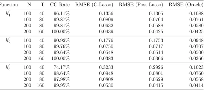
For C-lasso estimators, since there are three different groups each involving parametric and nonparametric estimators, I report both the maximum RMSE of ˆαk and ˆfk, and RMSE of ˆα
and ˆf, where ˆα≡( ˆα1,αˆ2, ...,αˆK0) and ˆf ≡( ˆf1,fˆ2, ...,fˆK0). Denote the number of repetitions
as M. The maximum RMSE of ˆα is defined as
max{RMSE}αˆ ≡ 1 M M X m=1 s max 16k6K0 αˆk,m−α 0 k 2 F
where ˆαk,m denotes the estimated parametric parameters ofkth group inmth repetition and
α0
k is the corresponding true value. Similarly, the maximum RMSE of ˆf is
max{RMSE}fˆ≡ 1 M M X m=1 s max 16k6K0 ˆ fk,m−fk0 2 2
where ˆfk,m and fk0 are defined similarly. We further define RMSE of ˆα and ˆf as
{RMSE}αˆ ≡ 1 M M X m=1 v u u t K0 X k=1 αˆk,m−α 0 k 2 F {RMSE}fˆ≡ 1 M M X m=1 v u u t K0 X k=1 ˆ fk,m−fk0 2 2
For post-Lasso estimators ˆαGˆ and ˆfGˆ, and oracle estimators ˆαG0 and ˆfG0, I similarly define
maximum RMSE and RMSE, where ˆαGˆ ≡( ˆαGˆ1,αˆGˆ2, ...,αˆGˆ
K0), ˆfGˆ ≡( ˆfGˆ1, ˆ fGˆ2, ...,fˆGˆ K0) and ˆ αG0 ≡( ˆαG0 1,αˆG02, ...,αˆGK00), ˆfG0 ≡( ˆfG01, ˆ fG0 2, ..., ˆ fG0 K0 ).
The main results are reported in Table 1.2 and 1.3. I discuss Table 1.2 first. When T
is relatively small (T = 60), the classification error is comparatively large. Around 25% (N = 90) or 20% (N = 180) of individuals are classified into wrong groups. Consequently, the maximum RMSE of ˆα, ˆf and ˆαGˆ, ˆfGˆ are considerable compared with that of the oracle
estimators. However, as T increases, the classification error shrinks quickly. For the case
N = 90, T = 90,N = 180, T = 90 and N = 270, T = 90, more than 90% of individuals are assigned the correct group identity. As a result, the maximum RMSE of C-lasso and post-lasso estimators decrease. When I further considerN = 180, T = 180 andN = 270, T = 180, the classification errors are only 1.2% and 0.2% respectively, and the RMSE of C-lasso and post-lasso estimators are almost the same as that of the oracle estimators. If I increaseT to 270 and consider N = 270, I achieve almost 100% correct classification. Consequently, the RMSE of C-lasso, post-Lasso and oracle estimators are of no difference. In Table 1.3, I get similar results.
By carefully comparing the results in Table 1.2 and 1.3, I further find that most of RMSE of C-lasso and post-lasso estimators could be attributed to the maximum RMSE of them.
T able 1.2: RMSE (Maxim um) of C-Lasso and p ost-Lasso Estimators in DGP 1 N T % of correc t Classification C-Lasso P os t-Lasso Oracle Maxim um RMSE of ˆα Maxim um RMSE of ˆf Maxim um RMSE of ˆαˆG Maxim um RMSE of ˆfˆG Maxim um RMSE of ˆ αG 0 Maxim um RMSE of ˆf0G DGP 90 60 76.9 0.557 0.384 0. 556 0.384 0.108 0.112 90 90 90.7 0.258 0.235 0.260 0.236 0.090 0.104 180 60 80.8 0.462 0.344 0.462 0.341 0.080 0.100 180 90 94.1 0.182 0.153 0.182 0.153 0.065 0.085 180 180 98.8 0.062 0.062 0.062 0.062 0.045 0.051 270 90 94.0 0.191 0.148 0.190 0.147 0.052 0.054 270 180 99.8 0.038 0.037 0.038 0.037 0.036 0.036 270 270 99.99 0.030 0.032 0.030 0.032 0.030 0.032
T able 1.3: RMSE of C-La sso and p ost-Lasso Estimators in DGP 1 N T % of correc t Classification C-Lasso P os t-Lasso Oracle RMSE of ˆα RMSE of ˆf RMSE of ˆαˆG RMSE of ˆfˆG RMSE of ˆ αG 0 RMSE of ˆf0G DGP 90 60 76.9 0.598 0.417 0. 597 0.416 0.131 0.152 90 90 90.7 0.290 0.267 0.292 0.267 0.110 0.134 180 60 80.8 0.491 0.366 0.491 0.365 0.097 0.125 180 90 94.1 0.199 0.170 0.198 0.170 0.078 0.106 180 180 98.8 0.079 0.082 0.080 0.082 0.055 0.068 270 90 94.0 0.205 0.164 0.205 0.162 0.062 0.075 270 180 99.8 0.045 0.053 0.045 0.053 0.043 0.052 270 270 99.99 0.036 0.045 0.036 0.045 0.036 0.045 28
1.4.3
Comparison with Complete Homogeneity and
Heterogene-ity
To further illustrate the advantages of C-lasso and post-Lasso estimators over complete parameter homogeneity or complete parameter heterogeneity, I compare the results of the three different approaches.
To make the approaches comparable, I define RMSE of C-lasso estimators in a different way. {RMSE}ind ˆ β ≡ 1 M M X m=1 v u u t 1 N N X i=1 ˆ βi,m−βi0 2 F {RMSE}ind ˆ h ≡ 1 M M X m=1 v u u t 1 N N X i=1 ˆ hi,m−h0i 2 2
where ˆβi,m and ˆhi,m denotes the estimated parametric and nonparametric parameters of
individuali in mth repetition using C-lasso.
For post-lasso and oracle estimators, I similarly define {RMSE}ind ˆ βGˆ, {RMSE} ind ˆ hGˆ and {RMSE}ind ˆ βG0, {RMSE} ind ˆ hG0, respectively.
If we assume individual share the same parameters, I denote the corresponding defined RMSE of parametric and nonparametric estimators as {RMSE}ind
ˆ
βho and {RMSE}
ind ˆ
fho. If we allow for complete parameter heterogeneity, I use{RMSE}ind
ˆ
βhe and {RMSE}
ind ˆ
fhe.
The results are reported in Table 1.4. Under complete parameter homogeneity, the model is misspecified. {RMSE}ind
ˆ
βho and {RMSE}
ind ˆ
fho don’t change much as N and T vary. While under complete parameter homogeneity, we fail to account for the group structure. WhenT is comparatively small (T = 60), C-lasso and post-lasso estimators don’t necessarily outperform those under complete parameter homogeneity and heterogeneity. However, as long asT is large enough (T = 90,180,270), C-lasso and post-lasso estimators perform much better.
T able 1.4: Comparison with Complete Homogeneit y and Heterogeneit y in DGP 1 N T % of correct Classification C-Lasso P ost-Lasso Orac le Homogeneit y Heterogeneit y RMSE of ˆβ RMSE of ˆh RMSE of ˆβˆG RMSE of ˆhˆG RMSE of ˆβG 0 RMSE of ˆhG 0 RMSE of ˆβho RMSE of ˆhho RMSE of ˆβhe RMSE of ˆhhe DGP 90 60 76.9 0.381 9.419 0.551 0.396 0.075 0.088 0.818 0.580 0.500 14.099 90 90 90.7 0.286 0.288 0. 330 0.257 0.063 0.077 0.818 0.579 0.388 0.403 180 60 80.8 0.374 13.155 0. 503 0.367 0.056 0.072 0.818 0.579 0.497 23.875 180 90 94.1 0.284 0.366 0. 300 0.223 0.045 0.061 0.817 0.579 0.394 0.531 180 180 98.8 0.184 0.183 0. 065 0.062 0.032 0.039 0.817 0.578 0.268 0.268 270 90 94.0 0.286 4.159 0. 323 0.221 0.036 0.044 0.817 0.578 0.394 6.230 270 180 99.8 0.181 0.190 0. 054 0.047 0.025 0.030 0.817 0.578 0.267 0.282 270 270 99.99 0.146 0.149 0. 024 0.027 0.021 0.026 0.817 0.578 0.217 0.221 30
1.4.4
Comparison with Misspecified Parametric model
In terms of classification, there is a concern that it might not be necessary to use semi-nonparametric models, because we might still achieve good classification even the model is misspecified as fully parametric.
To address this concern, I compare the classification errors of two different models: the true model and misspecified parametric model.
We first use DGP 1 as before. The results are shown in Table 1.5. The classification errors of the true model are always smaller than those of the misspecified model.
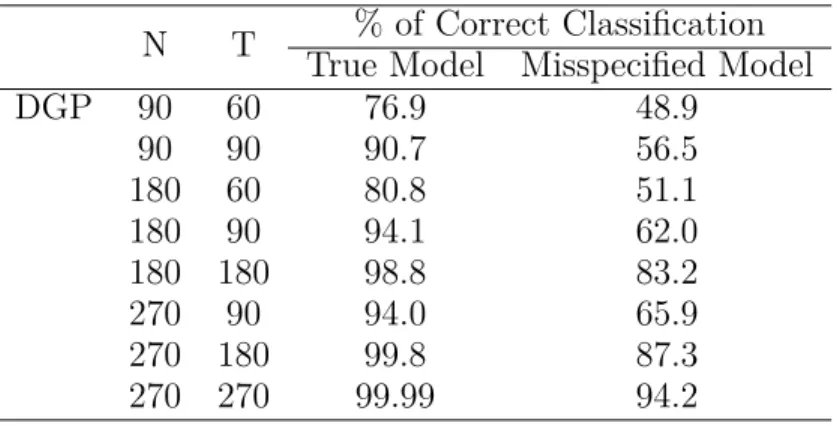
Table 1.5: Comparison with Misspecified Parametric Model in DGP 1
N T % of Correct Classification True Model Misspecified Model DGP 90 60 76.9 48.9 90 90 90.7 56.5 180 60 80.8 51.1 180 90 94.1 62.0 180 180 98.8 83.2 270 90 94.0 65.9 270 180 99.8 87.3 270 270 99.99 94.2
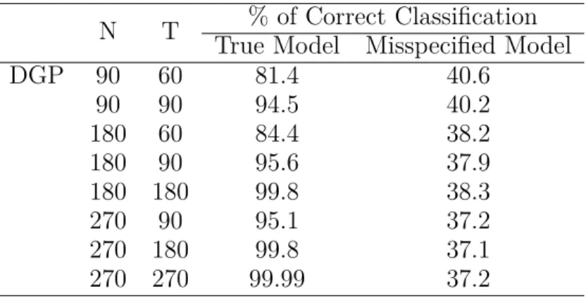
As T increases, the classification error of the misspecified model decreases, so one might conclude that it is still plausible to do classification using the misspecified model. However, under certain circumstances, the classification error of the misspecified model is large and does not improve even as T increases. To illustrate this idea, I consider a new model and DGP 2:
where h0i(x) = cos(2πx) if i∈G0 1 cos(4πx) if i∈G0 2 cos(6πx) if i∈G0 3
The other setting are the same as DGP 1. Then the misspecified parametric model is
yit=µi+xitφi+uit
After simple calculation, we could see that for individuals from different groups, the parameters are the same under the misspecified model, thus it is theoretically impossible to classify individuals into correct groups. The simulation results are shown in Table 1.6. With the misspecified model, the percentage of correct classification is at most 40.6% and doesn’t increase as T increases. Considering that with three equally-sized groups, there is at least 33.3% correct classification under suitable permutation, the error almost achieves its upper bound. On the contrary, with nonparametric model, I could still achieve good classification and the classification error shrinks as T increases.
Table 1.6: Comparison with Misspecified Parametric Model in DGP 2
N T % of Correct Classification True Model Misspecified Model DGP 90 60 81.4 40.6 90 90 94.5 40.2 180 60 84.4 38.2 180 90 95.6 37.9 180 180 99.8 38.3 270 90 95.1 37.2 270 180 99.8 37.1 270 270 99.99 37.2 32