Eddy-resolving simulations of the flow around a vertical tail plane

around a vertical tail plane

Andrea Masi

Department of Engineering

University of Cambridge

This dissertation is submitted for the degree of

Doctor of Philosophy

I hereby declare that, except where specific reference is made to the work of others, the contents of this dissertation are original and have not been submitted in whole or in part for consideration for any other degree or qualification in this, or any other university. This dissertation is my own work and contains nothing which is the outcome of work done in collaboration with others, except as specified in the text and Acknowledgements. This dissertation contains fewer than 65,000 words including appendices, bibliography, footnotes, tables and equations and has fewer than 150 figures.

Andrea Masi October 2017

The PhD journey would not have been possible without the support of many people. I would like to acknowledge my supervisor, Professor Paul Tucker, who has always shown great enthusiasm towards my project. I would like to thank him for his invaluable technical advice, encouragement and support, and for being available at any time during the year. His extra financial assistance during the later stages of my thesis is also greatly appreciated. I would like to thank my industrial advisor, Mr Jerry Benton, who has guided me throughout my experience at Airbus, always keeping an eye open to my academic activities at Cambridge. Jerry’s industrial expertise has no equals, and I consider myself privileged to have had such a supervisor.

The project is part of the ANADE (Advances in Numerical and Analytical tools for DEtached flow) consortium, with funding coming from the European Commission under the Marie Curie Actions. I am very grateful to the consortium, and notably to Professor Eusebio Valero, for their support. The consortium has given me the unique opportunity to work in close collaboration with other PhD students and researchers outside of the Cambridge environment. In particular, I would like to thank Maria Chiara Iorio, Andrea Resmini, Chris Hennekinne, Dirk Ekelschot, Bastien Jordi, and David Vallespin, not only for their professional collaboration but also for the great time spent together during the unforgettable ‘ANADE trips’, and the friendship that we have established. ANADE has also given me the opportunity to spend time at DLR in Germany. I would like to acknowledge Dr Axel Probst for his help and the interesting discussions we have had.

The Cambridge CFD group has been an exciting environment in which to learn and work towards the best results, and I would like to thank the whole research team for this. In particular, Jiahuan Cui and Ashley Scillitoe have been always very collaborative and I thank them for their insights into the research. I would also like to thank Hardeep Kalsi, Bryn Ubald, Ahmed Al-Shabab, Iffi Nakavi, James Tyacke, and Rao Vadlamani for the interesting discussions. People in the lab have certainly made the time in Cambridge more enjoyable. In particular, I am glad I have shared good moments with Girish Nivarti, Camille Bilger, and Carlo Quaglia, both in the lab and outside. They made my stay in Cambridge memorable, and I hope our lives will intersect again in the future. College life was also unforgettable. During

the last three years, I have met many people, from different countries, and with completely different backgrounds. Darwin College helped me develop personality and soft skills, giving me the chance to escape from the ‘Engineering bubble’. I would like to thank everyone who has contributed to this, during discussions, laughs, and drinks at ‘DarBar’. I much appreciate the friendship of Victoria Bartels and Charissa Varma, two incredible personalities who have always been available to listen, give advice and also spend fun times together.

Fifteen thousand miles! This is approximately the distance I have covered during the last three years, commuting from Cambridge to Bristol. At Airbus I have worked in a challenging and competitive industrial environment. I would like to thank the EGDCU team of Airbus, notably the PhD students and researchers. My colleague and friend Feng Zhu has always shown great interest in my research, and has given interesting inputs to the study. He has also hosted me many times during my visits to Bristol, and I will always be grateful for this. Many thanks also to Christian Agostinelli, Giuseppe Trapani, Giovanna Ferraro, Jean Demange, Simone Simeone, and Gabriele Mura for creating an enjoyable research environment. The first house-share experience in Bristol was memorable, especially due to the presence of my friends Jordi Bayer Alsina, Luisa Jolin Rubio, and Alessandro Saturni. Leaving Bristol was not easy after having spent a year with them. I am also grateful to Chris Curran and Sonia Richardson for their friendship and hospitality in Bristol. I would like to thank also Hansel Williams, the brightest light in the darkest period of my PhD. I thank him for his motivation and support. He taught me how to avoid procrastination and overcome drama.

Moreover, I would like to thank my friends Domenico De Fazio and Antonella Emili. Life and study circumstances have brought us to the same city again, and I am grateful to them for the great time spent together and for their encouragement and hospitality. They have always been ready to give me support when needed. Furthermore, I would like to thank those friends that are always there for me, and make life easier and better, notably Silvia Erario, Elena Monticelli, Rafael Narvaez Gracia, Kiliana Vink, Collegio Einaudi’s people, Valentina Corrado and ‘gli Storti’ of Toulouse.

The PhD course has been a great experience, despite some moments of discouragement that have been successfully overcome. This has been possible thanks especially to the endless support of my family. They keep saying that I am their pride, but they cannot express how important they have been throughout my studies. I will be grateful to them forever.

Andrea Masi October 2017

Enhancing the ability of engineers to predict the flow around the Vertical Tail Plane (VTP) of an aircraft generates important benefits to the aviation industry. For common multi-engine commercial airliners, the size of the VTP is driven by a particular flight condition - loss of an engine during take-off and low speed climb. Nowadays, Computational Fluid Dynamics (CFD) is the main tool used by engineers to assess VTP flows. However, due to uncertainties in the prediction of VTP effectiveness, aircraft designers keep to a conservative approach, which may risk oversizing of the tail plane, thus adding more resistance to the flight. Uncertainties emerge from difficulties in predicting the massive separation that occurs on the swept tail when it is approached by a flow at high incidence. Furthermore, the deployment of the control surface (the rudder) over the tail plane and the skewed flow along the span increase the CFD challenges. Improved predictive capabilities of the flow around VTPs would enable a more optimal design approach with potential resultant weight and drag savings.

The correct prediction of flow separation is the main driver of this study. Currently, the industry uses steady Reynolds-Averaged Navier-Stokes (RANS) simulations for or the assessment of VTPs flow. In order to assess RANS performance, the study of a flow detaching from a backward rounded ramp is performed in this thesis. The flow is skewed as it would be on the surface of a VTP. RANS simulations are compared to highly-resolved Large-Eddy Simulations (LES), also performed in this work. The analysis shows that, even though RANS may predict the onset of flow separation correctly, they completely miss the location of flow reattachment over the ramp, and this affects the whole flow solution. Moreover, in the LES the flow features a strong anisotropy at the onset of separation, difficult to be captured by RANS. The analysis shows that RANS cannot predict the same level of production of turbulent kinetic energy in the detached flow region, discouraging flow mixing, and delaying flow reattachment and recovery. A hybrid RANS/LES carried out on the same test case shows the benefits of using eddy-resolving simulations for detached flows. The prediction of the locations of the separation and reattachment points differs by only 1% from the highly-resolved simulation.

The VTP investigation carried out in this thesis uses a wind tunnel model tested at Airbus. The study starts with steady RANS approaches for different turbulence models. RANS simulations produce acceptable results for the flow at low incidence levels. On the contrary, at high incidence, when flow separation occurs RANS methods fail and it is not possible to assess the aerodynamic characteristics of the VTP. The second step of the research consists of using unsteady RANS (URANS) simulations for VTP flows at high sideslip angles. The introduction of time-accuracy brings important benefits. Nevertheless, the results still show some inaccuracies, especially in the local prediction of the pressure distribution over the surfaces of the model (around 20% error).

Finally, restarting from the flow solutions obtained by URANS simulations, higher fidelity hybrid RANS/LES techniques in the form of Delayed Detached-Eddy Simulations (DDES) are used to assess the characteristics of the separated flow around the tail plane. Results show a remarkable improvement of the flow solution. The pressure distribution matches experimental results favourably, and this translates into an improved prediction of the aerodynamic loads over the VTP (3-7% error with respect to experimental measurements). This leads towards a new strategy for the assessment of the flow over aircraft VTPs, amounting to an important contribution to the design of future aircraft.

List of figures xv

List of tables xxi

Nomenclature xxiii

1 Introduction 1

1.1 A reasonable growth . . . 1

1.2 Reduction of aircraft drag . . . 2

1.3 The design of the vertical tail plane . . . 4

1.3.1 Flow separation: a limiter of VTP efficiency . . . 5

1.4 Use of Computational Fluid Dynamics in aeronautics . . . 6

1.5 Structure of the thesis . . . 10

2 Literature review 13 2.1 Introduction . . . 13

2.2 Air-flow characteristics over vertical tail planes . . . 14

2.3 CFD for VTP flow assessment . . . 21

2.3.1 RANS simulations . . . 23

2.3.2 LES . . . 29

2.3.3 Hybrid RANS/LES . . . 32

2.4 Conclusions and objectives of the thesis . . . 39

3 Numerical methods 41 3.1 Introduction . . . 41

3.2 Governing equations . . . 42

3.3 Finite Volume Method . . . 44

3.3.1 Central scheme for spatial discretization . . . 45

3.4.1 Time-marching method for steady-state problems . . . 47

3.4.2 Dual time-stepping for unsteady problems . . . 49

3.5 Hybrid RANS/LES in TAU . . . 50

3.6 Control of the artificial dissipation . . . 52

3.7 Low-Mach number treatments . . . 54

3.8 Data analysis . . . 55

3.8.1 Monitoring of the residuals for steady-state simulations . . . 55

3.8.2 Temporal-averaging for unsteady simulations . . . 56

3.8.3 Visualising turbulence . . . 56

3.8.4 Computation of the forces and moments over the aircraft model . . 57

3.9 Computer resources . . . 59

4 Separation of a skewed boundary layer: an idealisation of VTP dynamics 61 4.1 Introduction . . . 61

4.2 The test case . . . 62

4.2.1 The mesh . . . 63

4.2.2 Inflow and boundary conditions . . . 64

4.3 Highly-resolved LES with crossflow . . . 67

4.3.1 Overall view and major characteristics of skewed flow . . . 67

4.3.2 Velocity and Reynolds-stress profiles . . . 72

4.4 RANS with crossflow . . . 76

4.4.1 Overall view and major characteristics . . . 76

4.4.2 Velocity profiles . . . 79

4.5 Production and dissipation of turbulent kinetic energy . . . 82

4.6 Hybrid RANS/LES with crossflow . . . 86

4.7 Conclusions . . . 89

5 Steady and unsteady RANS simulations 91 5.1 Introduction . . . 91

5.2 The VTP model . . . 92

5.3 Steady RANS simulations . . . 98

5.3.1 Steady results for VTP without rudder deflection . . . 98

5.3.2 Steady results for the VTP with rudder deflection . . . 101

5.4 Unsteady RANS simulations . . . 104

5.4.1 Unsteady results for VTP without rudder deflection . . . 105

5.4.2 Unsteady results for VTP with rudder deflection . . . 108

5.5 Conclusions . . . 111

6 Eddy-resolving simulations 115 6.1 Introduction . . . 115

6.2 Mesh refinement . . . 116

6.3 Flow and numerical parameters . . . 118

6.4 Results . . . 119

6.4.1 Overall flow characteristics . . . 119

6.4.2 Predictions of the aerodynamic loads . . . 125

6.4.3 Shape of the turbulence and validity of turbulence modelling . . . . 131

6.4.4 Assessment of the behaviour of the DDES delay function . . . 133

6.5 Cost of the simulations and overall considerations . . . 135

6.6 Conclusions . . . 136

7 Concluding remarks and recommendations for future work 139 7.1 Conclusions . . . 139

7.2 A strategy for the correct VTP flow assessment . . . 140

7.3 Recommendations for future work . . . 142

Appendix A Reynolds-Averaged Navier-Stokes Equations 145 A.1 Navier-Stokes Equations . . . 145

A.2 The Reynolds equations . . . 148

A.2.1 The continuity equation in Reynolds form . . . 149

A.2.2 Momentum equations in Reynolds form . . . 150

A.2.3 The energy equation in Reynolds form . . . 150

A.3 The problem of the closure . . . 151

A.4 Filtering the equation for Large-Eddy simulations . . . 151

Appendix B Turbulence models 153 B.1 The Spalart-Allmaras turbulence model . . . 153

B.2 The Menter-SST turbulence model . . . 154

B.3 The SSG/LRR-ω turbulence model . . . 156

Appendix C Validation of LES on the backward ramp without crossflow 159 Appendix D Grid convergence studies 165 D.1 Backward rounded step . . . 165

Appendix E Wind tunnel measurements 171

E.1 Data acquisition . . . 171 E.2 Aerodynamic corrections . . . 172

1.1 Trend of RPKs (in trillion US dollars) over the years. [8] . . . 2

1.2 Rear fuselage of the Airbus A380 aircraft. Photo courtesy of Airbus. . . 3

1.3 Scheme of the forces and moments on the aircraft when an engine fails during take-off or climb. . . 5

1.4 Scheme of the forces and moments on the aircraft in the presence of cross-wind at landing. . . 6

1.5 CFD in aircraft design [117]. . . 8

1.6 Turbulence modelling hierarchy [30]. . . 10

2.1 Aircraft vertical tail plane (VTP). . . 16

2.2 Velocity distribution of a boundary layer in the presence of an adverse pressure gradient (image from www.thermopedia.com accessed on 12 August 2016). . . 17

2.3 Structure of three-dimensional boundary layer [31]. . . 17

2.4 (a) Separation profile emanating from a separation point. (b) Separation surface emanating from a separation line [103]. . . 18

2.5 (a) Reattachment profile emanating from a separation point. (b) Reattachment surface emanating from a separation line [103]. . . 18

2.6 Flow visualization over a VTP atβ =0◦andδr=40◦[91]. . . 19

2.7 Mid-span flow visualization over the rudder of a VTP atβ=0◦andδr=30◦. Separation along the rudder surface. Photo courtesy of Airbus. . . 20

2.8 Flow visualization over a VTP atβ =20◦andδr=0◦[76]. . . 20

2.9 Schematic of a section of the VTP . . . 21

2.10 Use of CFD for the aerodynamic design of an Airbus A380 aircraft [2]. . . 22

2.11 Surface pressure distribution on the NDF hump. Comparison of different turbulence models results with experimental data [67]. . . 26

2.13 Schematic representation of the main flow features of the cube, Iaccarinoet

al. [50]. . . 29

2.14 Grid requirements against Reynolds numbers for a flow around a wing section of a span equal to the wing chord. Re-adapted from Tucker [109]. . . 31

2.15 Sketch of flow regions around an aerofoil in rotor downwash during hover, Spalart [100]. . . 33

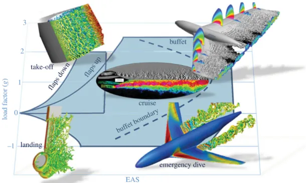
2.16 Generic flight envelope of a civil transport aircraft, with examples of hybrid RANS/LES simulations, Decket al. [30]. . . 36

2.17 Visualization of the turbulent structures of the flow detaching from the spoilers over an aircraft wing [43]. . . 36

2.18 Visulaization of the turbulent structures of the separated flow past the wing, Sartoret al. [90]. . . 37

2.19 Time-averaged wing pressure distribution at six spanwise stations of the wing of the CRM, Waldmannet al. [119]. . . 38

3.1 Contol volumes around pointsP(j1)andP(j2)[32]. . . 45

3.2 Energy spectrum obtained by incomptressible HYDRA LES without SGS model (readpated from Cui [27]). The experiment data is by Comte-Bellot [23]. . . 53

3.3 Turbulent kinetic energy spectra for the DIT case. Experiment vs. TAU DDES. 53 3.4 Lumley triangle showing limits of invariantsη andξ, Hamiltonet al.[45]. 58 3.5 Pressure force acting on a boundary face (re-adapted from [32]). . . 59

4.1 Analogy between VTP and backward rounded step. . . 62

4.2 Duct with backward rounded step. . . 63

4.3 Grid spacing in wall units and aspect ratio∆x/∆yalong the bottom wall [13]. 65 4.4 Flow-snapshots of the inflow for the backward rounded map test case, orga-nized in a turbulent box. Inflow data was received from Lardeau [57]. . . . 65

4.5 Mean velocity in streamwise direction. Inflow data was received from Lardeau [57]. . . 66

4.6 Turbulent boundary (characteristic displacement thicknessRe_θ ≈1190) of the inflow [13]. Comparison with DNS data [54]. . . 66

4.7 Source term in thez-momentum equation. . . 67

4.8 LES: Time-averaged flow along the duct. . . 68

4.9 Skin-friction lines on the wall of the backward ramp. . . 69

4.10 Skin-friction lines on the wall of the backward ramp. Zoom on separation and reattachment lines. . . 69

4.11 Instantaneous streamwise velocity. . . 70

4.12 Isosurface of theQ-criterion coloured by streamwise velocity. . . 70

4.13 Streamline contours of the time-averaged and spanwise-averaged flow field in the recirculation region. . . 71

4.14 Magnified streamlines. . . 71

4.15 Distributions of pressure and skin friction coefficients along the lower wall. 72 4.16 Mean velocity profiles . . . 74

4.17 Reynolds stresses profiles. . . 75

4.18 Contour of the flatness parameterA. . . 76

4.19 Lumley triangles of the flow in the recirculation region, withy/H<1.5. . . 76

4.20 RANS: flow along the duct. . . 77

4.21 Pressure coefficient over the lower wall of the duct computed by LES and RANS. . . 78

4.22 RANS: mean velocity profiles . . . 80

4.23 Reynolds stresses profiles: LES vs. RSM-RANS. . . 81

4.24 Production of turbulent kinetic energy contours. . . 83

4.25 Dissipation rate of turbulent kinetic energy contours. . . 84

4.26 Production and dissipation of TKE forx/H=1.5. . . 85

4.27 TKE profiles along the ramp. . . 85

4.28 Hybrid RANS/LES: flow along the duct. . . 86

4.29 Hybrid RANS/LES: flow recirculation region. . . 86

4.30 Pressure coefficient over the lower wall of the duct computed by LES and hybrid RANS/LES. . . 87

4.31 Hybrid RANS/LES: mean velocity profiles . . . 88

4.32 Hybrid RANS/LES: production of turbulent kinetic energy contours. . . 89

5.1 Assembly of the model in the wind tunnel. Photo courtesy of Airbus. . . 93

5.2 Sections of cuts of the VTP. . . 94

5.3 The computational domain. . . 94

5.4 2D sections of the VTP with a planez=const. . . 95

5.5 Aerodynamic loads generated by the VTP. . . 96

5.6 Surface mesh of the wind tunnel model. . . 97

5.7 RANS - Convergence of density residuals and sideforce: δr =0◦, β = 0◦, ...,20◦. . . 98

5.8 RANS - Flow visualizations forδr=0◦. Top: suction side. Bottom: pressure side. Streamlines onC pcontours (RSM turbulence model). . . 99

5.9 RANS - Pressure coefficient for four sections of cut obtained forδr=0◦and

β =0.17◦(RSM turbulence model). . . 100

5.10 RANS - Convergence of density residuals and sideforce: δr =30◦, β ≈ 0◦, ...,20◦. . . 101

5.11 RANS - Flow visualizations for δr =30◦. Top: suction side. Bottom: pressure side. Streamlines onC pcontours (RSM turbulence model). . . 102

5.12 RANS - Pressure coefficient for four sections of cut obtained forδr =30◦ andβ =0.17◦(RSM turbulence model). . . 103

5.13 URANS - Flow visualizations forδr=0◦andβ=14◦(averaged skin-friction lines, Menter SST turbulence model). . . 105

5.14 URANS - Pressure coefficient for four sections of cut obtained forδr =0◦ andβ =14◦. . . 106

5.15 URANS - Instantaneous Mach number contours with time-averaged stream-lines, forδr=0◦andβ =14◦. Section A-A (Menter SST). . . 107

5.16 URANS - Flow visualizations for δr =30◦ and β =10◦ (averaged skin-friction lines, Menter SST turbulence model). . . 109

5.17 URANS - Pressure coefficient for four sections of cut obtained forδr =30◦ andβ =10◦. . . 110

5.18 URANS - Mach number contours with time-averaged streamlines forδr= 30◦andβ =10◦. Menter-SST turbulence model. Section A-A. . . 111

5.19 URANS - Isosurface of theQcriterion forδr=30◦ andβ =10◦. Menter-SST turbulence model. . . 112

6.1 Schematics of a section of VTP at high sideslip angle. . . 116

6.2 Syrface contours showing∆y+ for wall cell height. . . 117

6.3 Schematic of the grid refinement procedure [32]. . . 118

6.4 Mesh refinement in the target zone. . . 118

6.5 Flow visualizations forδr=0◦andβ =14◦for the averaged flow, showing skin-friction lines andC pcolour contours. Comparison SST-URANS vs. SST-DDES. . . 120

6.6 DDES - Instantaneous Mach number contours with time-averaged stream-lines, forδr=0◦andβ =14◦. Section A-Aη=0.7. . . 121

6.7 DDES - Instantaneous isosurface of theQ-criterion forδr =0◦andβ =14◦ coloured by streamwise velocity. . . 121

6.8 Flow visualizations forδr=30◦andβ =10◦for the averaged flow, showing skin-friction lines andC pcolour contours. Comparison SST-URANS vs. SST-DDES. . . 122

6.9 DDES - Instantaneous Mach number contours with time-averaged

stream-lines forδr=30◦andβ =10◦. Section A-A (η =0.7). . . 123

6.10 Comparison of URANS and DDES turbulent structures forδr =30◦ and β =10◦. . . 124

6.11 DDES - Pressure coefficient for four sections of cut obtained forδr=0◦and β =14◦. . . 126

6.12 DDES - Evolution of the side force coefficient with time,δr=0◦andβ =14◦. 127 6.13 DDES - Evolution of the yaw moment coefficient with time, δr =0◦ and β =14◦. . . 127

6.14 Comparison of the accuracy of the three CFD methods (δr=0◦andβ =14◦).128 6.15 DDES - Pressure coefficient for four sections of cut obtained forδr =30◦ andβ =10◦. . . 129

6.16 Comparison of the accuracy of the three CFD methods (δr=30◦). . . 130

6.17 Fourier Transform of the side force coefficient with respect to the Strouhal number. . . 131

6.18 Three snapshots of the flow solution forη =0.8. . . 131

6.19 Flatness parameter for a section of the flow field. . . 132

6.20 Lag between shear stresses and strains for a section of the flow field. . . 133

6.21 Isosurfaces of theQcriterion coloured by the delay function f_d . . . 134

6.22 Contour map of the delay function f_dforη=0.7. . . 135

7.1 Suggested strategy for VTP flow assessment. . . 141

A.1 Control volume fixed in space, with the fluid flow moving through it [10]. . 145

A.2 Reynolds decomposition. . . 148

B.1 SSG/LRR-ω Reynolds stress scheme. . . 156

C.1 Pressure coefficientC pobtained by LES without crossflow and comparison with reference data by Bentalebet al.[13]. . . 160

C.2 Validation velocity profiles. . . 161

C.3 Validation velocity profiles. . . 163

D.1 Grid independence study on RANS mesh for the backward rounded ramp.u velocity contours and streamlines. . . 166

D.2 Comparison of the flow velocity profiles obtained on the baseline and refined grids. . . 167

D.4 Flow visualization for the refined mesh forβ =0◦. . . 168

D.5 Grid convergence study: baseline mesh vs. refined mesh,δr=0◦andβ =0◦. 169

E.1 Wind tunnel constraints. Picture courtesy of Airbus. . . 173 E.2 Wind tunnel support corrections. Picture courtesy of Airbus. . . 174

2.1 Reattachment point of the flow downstram a cube. Analysis of results from

Iaccarinoet al.[50]. . . 29

2.2 Landing gear study: wheel drag coeffiecient. Analysis of results from Hedges et al. [46]. . . 34

3.1 Smoothing coefficient used in the thesis. . . 47

3.2 Features of the clusters used for VTP simulations. . . 60

4.1 Grid sizes for LES, RANS and hybrid RANS/LES of the backward ramp. . 64

4.2 Comparison of separation and reattachment locations. . . 77

4.3 Comparison of separation and reattachment locations. . . 87

5.1 VTP geometry. . . 92

5.2 Sections of cut of the VTP. . . 92

5.3 RANS mesh details. . . 97

5.4 Loading on the VTP atβ =0.17◦andδr =30◦ . . . 104

5.5 Loading on the VTP forδr=0◦atβ =14◦. . . 107

5.6 Comparison between period and turbulent timescales in the SST and RSM URANS simulations. . . 108

5.7 Loading on the VTP atβ =10◦andδr =30◦ . . . 111

5.8 Accuracy vs. costs of URANS. . . 111

6.1 DDES mesh details. . . 118

6.2 DDES test cases. . . 119

6.3 Loading on the VTP atβ =14◦andδr =0◦ . . . 127

6.4 Loading on the VTP atβ =10◦andδr =30◦ . . . 128

6.5 Accuracy vs. costs of URANS and DDES. . . 136

B.1 Constants for the SA turbulence model. . . 154

C.1 Comparison of separation and reattachment locations. . . 160

D.1 Backward rounded ramp grids comparison (no. of grid points). . . 165 D.2 VTP grid comparison. . . 166

Roman Symbols

A First invariant (flatness parameter)

A₂ Second invariant

A₃ Third invariant

C_L Lift coefficient

C_D0 Zero-lift coefficient

C_Di Induced drag coefficient

C_DES DES coefficient

C f_y Side-force coefficient

CFL Courant number

Cmz Yaw moment coefficient

C p Pressure coefficient

E+ Normalised turbulent kinetic energy

f Frequency OR Body force (source term) in Navier-Stokes equations

f_d DDES delay function

Fy Force iny-direction (side-force)

IQ Quality index

k+ Normalised wavenumber

kL Wavenumber multiplied by the integral length scale

l_hyb Hybrid RANS/LES length scale

l_LES LES length scale

l_RANS RANS length scale

M∞ Free stream Mach number

M_z Moment inz-direction (yaw moment)

P_k Production of turbulent kinetic energy

Q Second scalar invariant of the velocity derivative tensor

Re Reynolds number St Strouhal number t_i Turbulent timescale t_p Unsteadiness period u x-velocity v y-velocity

V∞ Free stream velocity

w zvelocity

y+ Dimensionless wall distance

y_wall Wall coordinate

CFD Computational Fluid Dynamics

CPU Computer Power Unit

DDES Delayed Detached-Eddy Simulation

DES Detached-Eddy Simulation

ER Euler Region

FR Focus Region

HPC High-Performance Computing

IDDES Improved Delayed Detached-Eddy Simulation

LES Large-Eddy Simulation

MAC Mean Aerodynamic Chord

MPI Message Passing Interface

NS Navier-Stokes

RANS Reynolds-Averaged Navier-Stokes

RPK Revenue Passenger Kilometres

RSM Reynolds Stress Model

SA Spalart-Allmaras turbulence model

SST Menter Shear-Stress Transport model

TKE Turbulent kinetic energy

URANS Unsteady Reynolds-Averaged Navier-Stokes

VTP Vertical Tail Plane

Greek Symbols

αMA Stress-strain misalignment angle

β Sideslip angle

δr Rudder deflection angle

Introduction

1.1

A reasonable growth

Aviation has changed society dramatically in the last century, introducing new, efficient, and fast ways of transporting people and goods. The growth of air traffic in the last 50 years has been impressive and projections by the Advisory Council for Aeronautics Research in Europe (ACARE) show that this trend is likely to continue in the future [3]. Air traffic is already well-established in developed countries, with many routes connecting North America with Europe. However, nowadays developing markets, such as China, India, and Brazil, are participating more and more in the world economy, and air traffic is reflecting this. The number ofmega-citieswill increase within the next 20 years and air traffic is likely to increase in proportion to connect these hubs of the global economy [8]. Airbus, for example, has reported an analysis by the ICAO (International Civil Aviation Organization), showing that, since air transport began, Revenue Passenger Kilometres1 (RPKs) have doubled every 15 years, despite the economic crisis of 2008. Figure 1.1 shows that, In 2012, global RPKs were equal to 6.5 trillion US dollars, whereas in 2032 this amount will reach around 14 trillion US dollars. As a consequence, the global aircraft fleet will need to grow.

This forecast is promising not only for the world economy, but also for research and technological development. In fact, the aviation industry involves a lot of sectors which will see the benefits of common technological development. However, there are many challenges in terms of sustainability. The amount of greenhouse gas emissions will increase worryingly if aircraft manufactures do not try to reduce them through the use of advanced technologies. In addition, attention needs to be paid to acoustic pollution: airports will be busier and busier; new hubs will appear, and more people will be affected by aircraft noise. Furthermore,

Fig. 1.1 Trend of RPKs (in trillion US dollars) over the years. [8]

governments already impose high charges on air traffic, which could increase in the near future, possibly causing a shift of passengers towards cheaper transport systems over short distances, such as the train. The aviation industry must act now to achieve improvements in aircraft performance, therefore sustain reasonable growth.

1.2

Reduction of aircraft drag

Aircraft design is highly advanced. Thanks to research and development in the last century, manufacturers constantly try to improve the aircraft design, in order to sell competitive products. Fuel consumption is one of the most critical parameters of aircraft performance. Reducing the consumption of kerosene gives rise to two main advantages: a reduction in the emission of pollutant gases (NO_x andCO₂), and a cut in the operating costs. The aviation engine industry works hard to design efficient engines, but to reduce fuel consumption, first of all it is necessary to optimize the aerodynamic shape of the aircraft. Engines have to generate the thrust to sustain the aircraft in the air. The higher the resistance the aircraft generates in flight, the higher the thrust generated by the engines needs to be, and the higher the fuel consumption. For this reason, reducing aircraft drag, the force that opposes the motion of the aircraft though the air, is a top priority of the aviation industry.

Aerodynamic drag is a mechanical force generated by the interaction and contact of a solid body (the aircraft) with a fluid in motion (the air). In aircraft subsonic aerodynamics, drag comprises two contributions: the zero-lift drag and lift induced drag. The former is due to frictional resistance of the body passing through the air. The latter is caused by

the generation of lift. It is also called ‘drag due to lift’ because it only occurs on finite, lifting wings. For a lifting wing, there is a pressure difference between the upper and lower surfaces of the wing. Vortices are formed at the wing tips, which produce a swirling flow that is very strong near the wing tips and decreases towards the wing root. The wing’s local angle of attack is increased by the induced flow of the tip vortex, giving an additional, downstream-facing component to the aerodynamic force acting on the wing. The force is called ‘induced drag’ because it has been ‘induced’ by the action of the tip vortices.

In cruise conditions, drag contributions are almost equally divided among wing, fuselage, and nacelles (30% each), and 10% at the tail planes, equally split into 5% for the horizontal tail and 5% for the vertical tail [77]. This thesis studies a particular aircraft component -the Vertical Tail Plane (VTP), or vertical stabilizer. The installation of -the VTP on -the rear part of the fuselage requires high assembly complexity and significant mass. Figure 1.2 shows the rear part of the Airbus A380, the biggest passenger aircraft in the world. The VTP span is about 15 metres long and the geometric mean chord is approximately equal to seven metres. The photo gives a sense of how big these dimensions are compared to the human size. Therefore, one can imagine that this component generates a large drag. Being a crucial element for the manoeuvrability of the aircraft, the VTP has to be efficient and has to ensure safety, and no design errors are allowed. A smaller fin would help designers to accrue benefits in aircraft performance. To achieve this, it is necessary to improve current aerodynamic design capabilities.

1.3

The design of the vertical tail plane

In order to ensure manoeuvrability and control, aircraft are equipped with a flight control system. The flight control system consists of primary and secondary controls. Primary controls include the ailerons, the elevators, and the rudder and are mounted respectively on the wing, the horizontal, and the vertical tail planes. The ailerons control the roll of the aircraft, the elevators control the pitch, and the rudder governs the yaw. However, there are also coupled effects that the controls can generate by their activation. The throttle is also a primary control which acts on the thrust generated by the engine or engines. Secondary controls generally give the pilot finer control and can alleviate their workload. Some of the secondary controls are the elevator trim, the flaps, and the slats. This thesis focuses upon the vertical tail plane, which consists of two parts: one is fixed (the fin), and the other (the rudder) can rotate around a hinge axis. The conventional tail configuration for commercial airliners consists of fuselage-mounted tail planes, and both the horizontal and the vertical tails are anchored to the rear fuselage. This configuration shows high efficiency and increased manoeuvrability capabilities compared to other shapes.

The criteria that drive the design of the VTP are given in FAR Part 23.149 and FAR Part 25.149 (Federal Aviation Regulations) and have been summarized in several books of aircraft design. Torenbeek [104] identifies four requirements for the VTP:

a. the vertical tail plane must not stall as a result of an oscillation after deflection of the rudder or sudden engine failure;

b. after failure of the critical engine, multi-engined aircraft must remain controllable to ensure steady flight;

c. it should be possible to land transport aircraft in crosswinds up to 30 knots (55 km/h), and

d. the aircraft must possess positive directional and lateral static stability and short-period lateral/directional oscillation (Dutch roll) must be damped.

The condition of engine failure is the most critical if the VTP is to maintain control over the aircraft. The failure of an engine is most critical during take-off and climb, due to the low speed of the aircraft. In four engine configurations, such as the A380, the case of two-engine-failure is the most restrictive design condition. As Figure 1.3 shows, the failure of an engine causes a yawing moment which must be balanced through deflection of the rudder on the VTP. Due to the coupling of aerodynamic effects on the aircraft’s longitudinal and lateral planes, a minor effect of engine failure consists of a rolling moment, which must

be controlled by use of the wing ailerons. This particular flight condition determines the size of the VTP and the rudder efficiency; it might also affect the size of the ailerons on the wing.

Fig. 1.3 Scheme of the forces and moments on the aircraft when an engine fails during take-off or climb.

Crosswind landing is another particular flight condition that drives the size of the VTP. As sketched in Figure 1.4, a crosswind unbalances the aircraft, so the rudder must be used to balance the forces on the aircraft.

Finally, in order to have a symmetric flight in normal flight conditions, the section of the aerofoil of the VTP must be symmetrical.

1.3.1

Flow separation: a limiter of VTP efficiency

The flow around the aircraft generates forces and moments that sustain and control the aircraft. If the flow detaches from the aircraft surfaces, these forces and moments are generally reduced. The worst case consists of the stall of that flying surface, which then loses its efficiency. This is commonly known for the most important component of an aircraft, the wing. However, flow separation can also affect the vertical tail surfaces. For this reason, it is important to design all of the components of the aircraft in order to delay flow separation as much as possible. Moreover, it is necessary to understand when flow separation occurs, where the onset of detachment is, and how far the efficiency of the flying surfaces is

Fig. 1.4 Scheme of the forces and moments on the aircraft in the presence of crosswind at landing.

affected. At present the problem is that, due to current uncertainties in aerodynamic design and lack of experimental data at operative Reynolds numbers, aircraft designers tend to use a conservative approach in sizing the VTP. This is to ensure that, even if flow separation occurs earlier than predicted by design, it is possible to maintain the efficiency of the rudder control. If prediction methods can be improved, weight and drag savings could be achieved through the use of smaller VTPs. The objective of this thesis is to assess the flow around a VTP, validating computational methods that can provide an accurate answer to the problem of flow separation. The objective will be explained further in Chapter 2.

1.4

Use of Computational Fluid Dynamics in aeronautics

The criteria that must be followed to design a VTP define particular flow conditions, which include low speed (compared to general aircraft cruise speed), turbulence, and flow separation. Therefore, the assessment of VTPs flow is challenging and research is currently investing a lot of resources to address this task. This thesis suggests ways and opportunities to improve the design of tail surfaces through the use of novel numerical techniques in Computational Fluid Dynamics (CFD). Spalart and Bogue [96] observe that CFD is used not only in design conditions, but also in off-design conditions. Tucker [107] explains that CFD

is used in external aerodynamics, in cabin ventilation flows, and also in avionics, electronics, and fire management. CFD is a powerful tool in aerodynamic design and is widely used in the aviation industry. As we see in Figure 1.5, it takes its proper place in the design process. The ‘CFD Environment’ includes:

1. Geometry and CAD modelling: every test case that needs to be studied has to be represented via computed-aided design (CAD) software on a machine;

2. Grid generation: the geometry needs a mesh, which is a grid consisting of points that define subdomains of the flow;

3. Solver computation: the mesh is given to a solver, which implements some algorithms to compute the flow. The task of the solver is toresolveormodelthe Navier-Stokes equation, which will be presented later in the thesis, and

4. Post-processing: Once the solution has been obtained, it needs to be analysed and visualized.

Grid generation is considered as the bottleneck of CFD for many reasons, as explained by Voset al.[117]. First of all, meshing is usually a time-consuming task, which needs good precision. Often the process is not automated, and requires constant inputs from the user. For the VTP, challenging meshing areas are the intersection between the fuselage and the tails, and also the gap between VTP and fuselage in the case of rudder deflection. Secondly, the quality of the mesh needs to be constantly tested and the user must make sure that the results are not grid-dependent.

The computation performed by the solver needs to represent the physics of the flow around the VTP in design conditions. But why is this flow challenging for CFD simulations? The main challenge resides in the presence of flow separation. In fact, when the flow reaches the vertical tail surfaces with a high angle of attack, flow detachment can occur along the fin. Eventually, as the angle of attack increases, the tail surface can also stall, leading to loss of VTP efficiency. A massively detached flow is extremely unsteady and turbulent, and results in being very difficult to study with current industrial tools. Another location of flow separation for the VTP is the deflected rudder, and the flow tends to separate around the hinge axis. Hence, for this configuration, the tail plane has two different locations of flow separation, and CFD simulations are even more challenging.

Challenges also include the turbulent character of the flow. Most aerospace flows involve high Reynolds numbers and will typically have turbulent boundary layers over all surfaces. In 1964 physicist and philosopher Richard Feynman stated: “Turbulence is the last great unsolved problem in classical physics”. And, although many studies have been done on this

subject, the problem of characterizing turbulence is still open. In 1510, Leonardo made the first attempt to study fluid motion. Observing water, he wrote2:

”Observe the motion of the water surface, which resembles that of hair, that has two motions:

one due to the weight of the shaft, the other to the shape of the curls; thus, water has eddying motions,

one part of which is due to the principal current, the other to the random and reverse motion.”

Leonardo understood that the motion of a fluid can be divided into a mean part and a fluctuating part. The lack of mathematical tools did not enable him to formulate this principle, and several centuries had to pass before Reynolds would introduce the decomposition that bears his name (see Appendix A). Introducing the Reynolds decomposition in the Navier-Stokes equations and time-averaging leads the way towards the formulation of the Reynolds-Averaged Navier-Stokes (RANS) equations, which are the industry tool most widely used nowadays for computational aerodynamic design (see Appendix A). In the RANS equations, new unknowns appear - the ‘Reynolds stresses’ - and modelling of the turbulence is necessary for the closure of the system of the equations.

Another technique used in CFD is Large-Eddy Simulation (LES). Its formulation derives from another kind of mathematical decomposition (see Appendix A). The main idea behind LES consists of resolvingthe large scales of turbulence within a flow, and modelling the small scales of turbulence. As will be discussed in Chapter 2, using LES for whole aircraft geometries is still computationally prohibitive.

Between RANS and LES, hybrid methods settle. Their scope is to combine the accuracy of LES for those flows which RANS cannot capture correctly with the simplicity of the RANS technique in regions where a more accurate simulation is not needed.

Figure 1.6 shows the classification of the CFD methods cited above in a pyramid organized with respect to the accuracy of the CFD technique. Steady and unsteady RANS methods are less accurate and more turbulence model-dependent, therefore they are at the bottom of the pyramid. However, relative to the other methods, their cost is low, hence the industry uses them as design tools. Hybrid RANS/LES and LES then follow. At the top of the pyramid, Direct Numerical Simulation (DNS) is found. This is the only CFD approach that does not need any sort of modelling, but its application on industrial cases is currently prohibitive, due to the level of grid and time refinement that is necessary.

Fig. 1.6 Turbulence modelling hierarchy [30].

In this thesis attention is paid to RANS, URANS, hybrid RANS/LES, and LES ap-proaches, with the aim of understanding how the aerodynamic prediction of the flow around a vertical tail plane can be improved.

1.5

Structure of the thesis

Chapter 2 presents a literature survey, which aims to understand the physics of the flow around aircraft stabilizers and which CFD methodologies may be successful (or not successful) for predicting VTP air-flow characteristics. This will help define the objectives of the thesis, together with a strategy for the assessment of VTP flows.

Chapter 3 illustrates the methodology used for the CFD analysis performed in this thesis, with special attention to eddy-resolving methods.

Chapter 4 presents the study of a three-dimensional boundary layer separating from a backward rounded ramp. Since the correct prediction of flow separation is key important for the assessment of the flow around a VTP, the test case studied in Chapter 4 highlights the reasons why industrial CFD methods, based on RANS approaches, fail to predict a detached flow. Eddy-resolving simulations will be also investigated.

Chapters 5 and 6 address the problem of CFD simulations over an aircraft VTP for different sideslip angles and two configurations of the rudder control (zero deflection and 30◦deflection) . Chapter 5 presents steady and unsteady RANS simulations, and highlights their accuracies and their limits with VTP flows at high incidence. In Chapter 6, the use of eddy-resolving simulations will be investigated.

Using the insights gained from the results chapter, in the final chapter a strategy for the correct VTP flow assessment is suggested.

Literature review

2.1

Introduction

In the public literature, few CFD studies of vertical tail planes are available, although many studies of aircraft wing-body configurations have been published. However, the flow topology around the VTP is quite different from that observed around a wing. This is due to the fact that wings and vertical fins have to satisfy different design criteria and performance requirements. Generally, for a commercial two-engine (or four-engine) aircraft, the VTP consists of a low-aspect-ratio wing, which is equipped with a movable control surface (the rudder), that is deflected when needed. Most wing-body CFD studies cover test cases at cruise speed (M_∞≈0.8), involving transonic flows and eventually the presence of shock waves. By contrast, as discussed in the introduction, in VTP design there is growing interest in CFD for low-velocity regimes (take-off or landing speeds), high sideslip angles, and deflected rudders.

This literature survey aims to understand the physics of the flow around aircraft stabilizers and which CFD methodologies may be successful (or not successful) for predicting VTP air-flow characteristics. Since VTP design conditions involve flows at high sideslip angles and/or high rudder deflections, the problem of flow separation is the main driver of this study, and we need to investigate how CFD tackles this problem in the current state of the art. To achieve this, the literature review covers RANS, LES and hybrid RANS/LES studies, discussing the applications that are relevant to this thesis. This will lead to the definition of the objectives of this work and the research strategy will be drawn.

A better understanding of the behaviour of the flow around a VTP can bring important improvements to aerodynamic design. First of all, the prediction of the pressure distribution, hence of the aerodynamic loads, can come closer to the measurements, and this would impact directly the sizing of the VTP. Moreover, a deep understanding of the separation mechanisms

on the VTP can lead to the design of more efficient active flow control devices1. In fact, today the industry is interested in the possibility of delaying or suppressing flow separation from aircraft surfaces, including the vertical fin and the rudder, through the use of passive and active flow control technologies, as explained by Abbaset al. [1, 2]. Hence a correct prediction of VTP flow is important for a useful outcome in the design of such systems. Furthermore, it would also be beneficial for the improvement of rapid-CFD methods, which are used in the preliminary conceptual design of an aircraft. Therefore, this research may open new scenarios for future work.

When can a CFD flow solution be considered good enough for VTP design? There is no straight answer to this question. In 1998, in a report from AIAA2 it was stated that “validation is the process of determining the degree to which a [CFD] model is an accurate representation of the real world from the perspective of the intended uses of the model” [5]. Unfortunately it is not possible to give a definite answer about the maximum allowable error from a CFD simulation with respect to experimental data. Aircraft manufacturers generally assess the validity and the accuracy of a CFD simulation based on the following criteria:

• examination of the iterative convergence of the numerical simulation;

• examination of the consistency of the CFD solution, in terms of comparison with previous or similar studies;

• examination of the convergence with respect to the mesh refinement of the computa-tional domain (if possible);

• comparison with experimental data, and

• examination of model uncertainties.

Therefore, these steps need to be followed in order to assess the validity of the flow solutions presented in this thesis.

2.2

Air-flow characteristics over vertical tail planes

Today, the most common VTP geometry chosen for civil aircraft consists of fuselage-mounted tail planes, which ensure a better response in controllability and manoeuvrability of the aircraft with respect to other configurations. The VTP, also known as stabilizer, is divided into two main components, that is, the fin, which does not move, and the rudder,

1_{Flow control devices prevent or delay flow separation over a flying surface.} 2_{American Institute of Aeronautics and Astronautics.}

which can rotate around the hinge line (see Figure 2.1a). The root of the VTP is connected to the fuselage (omitted in the picture); usually the tail is tapered, which means that the tip has a smaller chord with respect to the root. The sweep angle suggests a decomposition of the free stream flow velocityV∞into two components (Figures 2.1b):V⊥perpendicular to the leading

edge, andV_∥which is parallel to the leading edge. Therefore the flow is characterized by marked three-dimensionality, with a component of the velocity that runs along the span of the tail (spanwise).

As explained earlier, the design conditions of flow around VTPs involve high incidences, which may lead to flow separation. The problem of flow separation was firstly studied by Prandtl, in the formulation of the theory of boundary layers. As reported by Chang [74], Prandtl states flow separation occurs under two conditions:

• adverse pressure gradient along the flow path, and

• viscosity effects.

Flow separation cannot occur without viscosity. Prandtl proved this by looking at the flow in a channel; in the diverging part (where the adverse pressure gradient is present) the boundary layer tends to separate. The scientist did the same experiment by sucking away the boundary layer from the walls of the channel, showing that flow did not separate.

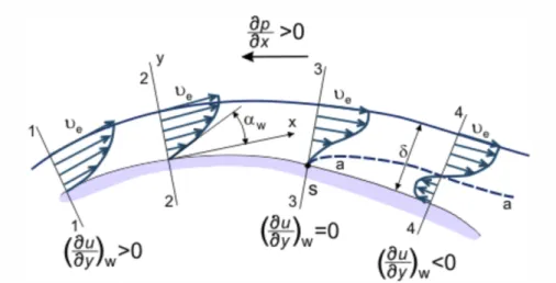
Figure 2.2 shows what happens in the boundary layer in the presence of an adverse (positive) pressure gradient, that is, the pressure increases in the flow direction. The adverse pressure gradient causes fluid particles in the boundary-layer to slow down at a greater rate than that is due to boundary-layer friction alone. The flow loses energy and the velocity distribution changes gradually from sections 1 to 4. In section 3, a point of inflection in the velocity profile appears. This stage, denoted by S, is the onset of separation. The flow evolves further and reverses, as shown in section 4. The dashed linea-adenotes the locus of the points where the velocity is null. The separation generates reverse flows and swirls.

For industrial geometries, flow separation is more complex due to the presence of three-dimensional boundary layers, as shown in Figure 2.3. The picture shows that the velocity distribution is given by two contributions: the streamwise profile and the crossflow profile. Flow separation over aircraft surfaces can be detected by looking at the skin-friction lines, as explained by Delery [31] and Suranaet al. [103]. When flow separation occurs, skin-friction lines show a mathematical singularity over the surface, converging or tending to converge towards a single line. By contrast, when the flow reattaches to the surface, the skin-friction lines diverge, redistributing sensibly on the surface. This is shown in figures 2.4 and 2.5 respectively. Skin-friction lines can also show the presence of vortical structures downstream

(a) VTP components.

(b) Flow decomposition over a VTP.

Fig. 2.2 Velocity distribution of a boundary layer in the presence of an adverse pressure gradient (image from www.thermopedia.com accessed on 12 August 2016).

of the separation. For these reasons, the use of skin-friction line plots from numerical computations is a method that can satisfactorily show the presence of separated flows.

Fig. 2.3 Structure of three-dimensional boundary layer [31].

Experimental observations and CFD simulations have shown that aircraft VTPs feature flow separation in the presence of a high sideslip angle of the flow and/or when the rudder control surface is deflected. For example, Seeleet al. [91] have recently performed a test campaign at the CalTech3Wind Tunnel, in which they assess the performance enhancement of a vertical stabilizer equipped with flow control devices. In the baseline experiment (without flow control devices), the authors present flow visualizations for a VTP at zero sideslip angle

Fig. 2.4 (a) Separation profile emanating from a separation point. (b) Separation surface emanating from a separation line [103].

Fig. 2.5 (a) Reattachment profile emanating from a separation point. (b) Reattachment surface emanating from a separation line [103].

and at different angles of deflection of the rudder. The flow is visualized through the use of tufts, which are small lengths of string attached to the surface at one end and frayed at the other. The tufts adhere to the tested surface if the flow is attached, whereas they detach from the surface if the flow is separated. Figure 2.6 shows that for about 40◦of rudder deflection (80% of its maximum extension), the flow topology over the fin is quite different from the one over the rudder. In fact, on the fin the flow is attached and the streamlines are parallel to the free-stream flow. Aft of the hinge, the tuft deflections show unevenness, which would suggest more disturbed flow due to separation. A similar study has been performed at Airbus, through the use of surface oil visualizations. Figure 2.7 shows the streamlines over a VTP at zero sideslip angle and 30◦rudder deflection. The streamlines reach the hinge-line and change direction feeding the vortex tip. A separation line is located along the rudder, running upwards along the span.

Varying the sideslip angle of the free-stream flow modifies the flow topology over the VTP, as derived from a wind tunnel test by Nicolosiet al.[76]. The authors study the flow around a vertical stabilizer at Reynolds number equal to 4.6·105(based on the mean chord), and sideslip angleβ =20◦. The flow speed is equal to 50 m/s. Figure 2.8 shows the VTP

configuration with tufts on the suction side surfaces. The flow is completely separated, as depicted by recirculation of the tufts.

Fig. 2.6 Flow visualization over a VTP atβ =0◦andδr=40◦[91].

From these experiments, we can identify two regions of flow separation on aircraft VTPs, that is, flow separation along the leading edge of the fin, and flow separation along the hinge line of the rudder. The former may occur when the free-stream flow reaches the fin at high sideslip angle, whereas the latter may occur when the rudder is deflected. For simplicity, Figure 2.9 shows a schematic of a 2D section of a VTP. The flow that reaches the VTP at incidenceβ splits into two parts. One passes over the pressure side down to the rudder, and

the other one contours around the leading edge of the fin and reaches the suction side. At high sideslip angles, the flow separates massively from the leading edge of the fin. If the flow reattaches on the tail, it convects down to the rudder, which is the second location of flow separation. On the VTP, the separation lines tend to be skewed along the span, toward the tip of the tail.

Fig. 2.7 Mid-span flow visualization over the rudder of a VTP at β =0◦ and δr =30◦.

Separation along the rudder surface. Photo courtesy of Airbus.

Fig. 2.9 Schematic of a section of the VTP .

2.3

CFD for VTP flow assessment

Having assessed the flow characteristics over aircraft VTPs, it is important to understand now how CFD can tackle the problem of separated flows on such industrial applications. However, the literature lacks test cases involving the combination of high sideslip angles and rudder deflection, hence information must be gathered from related literature in order to use the transferable knowledge from previous and current research. CFD is widely used in the aerospace industry, with a vast number of applications, extending from traditional design conditions to the off-design flow over peripheral components, as explained by Tucker [108]. Abbaset al. [2] describe the state of the art of numerical simulations for aerodynamic design at Airbus, one of the world’s major aircraft manufacturers. Figure 2.10 shows that CFD is used to design most aircraft components, including the tails. Moreover, aircraft designers are also becoming more interested in using CFD also for increasing the comfort of passengers, reducing engine noise, and improving cabin ventilation. This interest is growing significantly, consequently numerical simulations incur new challenges. A similar scenario is present at the other major aircraft manufacturer, Boeing, as described by Spalart and Venkatatarishnan [99] in a more recent publication.

RANS simulations can deliver results with a good compromise between accuracy and cost, at least in design conditions at cruise speeds. However, the same level of reliability is not achieved in off-design conditions involving, for instance, the deflection of the rudder on the VTP at low speeds. In the industry, priority to resolve these flows is given to steady RANS approaches, and generally 2-equations eddy-viscosity turbulence models are used for this task. Increased demand for accuracy has recently pushed CFD practitioners to investigate

Fig. 2.10 Use of CFD for the aerodynamic design of an Airbus A380 aircraft [2].

also Reynolds Stress Models (RSM, see Appendix B). The objective consists of trying to predict all local flow phenomena correctly, and the introduction of six transport equations (one for each Reynolds stress) in the turbulence model is thought to be beneficial for this task. Nevertheless, the computer time needed to resolve this set of equations increases considerably, with respect to simpler two-equation models. Hence, in the literature and in industrial practice, this has not yet been demonstrated for the flow around a VTP. Does the complexity of the turbulence model really add something more to the solution obtained by, for instance, a Menter-SST simulation? If so, at what cost? These questions are addressed in this thesis.

In aircraft design CFD is usually complimented by wind tunnel experiments, and vice-versa. Measurements continue to be a major means of providing aerodynamic information, and comparison (when possible) is still an important means of validating the numerical simulation. However, as explained by Tucker [111], wind tunnel tests for real industrial applications present many challenges. The main difficulty consists of reaching the Reynolds numbers typical of aircraft speeds and geometries, therefore experimentalists adopt geom-etry scaling and/or flow conditions scaling. Other limitations associated with wind tunnel experiments consist of the blockage effect of the wind tunnel, due to the presence of the walls, the presence of the structure that holds the model, the deformation of the model, due to

high pressures used to achieve high Reynolds numbers, the elevated cost of the models and experiments, and other factors that are presented in Appendix E. For these reasons, nowadays, CFD simulations, whatever their limitations, are becoming the favourite tool for aerodynamic design.

2.3.1

RANS simulations

Agarwal [4] reviewed CFD methods for whole-body aircraft simulations, focusing es-pecially upon steady RANS studies. At the end of the last century, Reynolds-averaged numerical simulations were cost-prohibitive. In less than 20 years, computer power has increased exponentially, reducing simulation costs significantly. The flow around an aircraft at cruise speed is reasonably well-predicted by RANS, which nowadays constitute the main design tool in industry. However, for some flow topologies, the gain in accuracy of steady RANS simulations has not been satisfactory, as explained by Spalart [94]. For instance, flow separation due to high incidence of the flow is still an open issue, and this is crucial for the correct prediction of the flow over VTPs.

Details of turbulence modelling for CFD can be found in references by Pope [81] and Wilcox [123]. A comprehensive review of turbulence models was performed by Leschziner and Drikakis [64]. In order to predict correctly the separated flow over a surface, it is necessary to model the near-wall shear-stresses and normal stresses correctly, as explained by Leschziner [63]. For 3D boundary layers, like on the VTP surface, all components of the shear-stress have to be detected. This influences locations of flow separation and reattachment dramatically.

Generally, turbulence models are grouped in the following branches:

• Linear Eddy-Viscosity Models (LEVM), which make use of the Boussinnesq approx-imation in order to close the system of equations. The Boussinnesq hypothesis (see Section A.3) proportionally links the flow Reynolds stresses and the flow shear stresses gradients through the eddy-viscosity [15, 81]. The models are usefully classified according to the number of transport equations they use, as discussed hereby:

– Algebraic models: the simplest models, designed for canonical flows not in-volving much separation. Algebraic models tend to predict excessive levels of eddy-viscosity, which results in difficulty in predicting the onset of flow separa-tion.

– One-equation models. The Spalart-Allmaras (SA) model [95] is the most investi-gated model of this category. It tends to delay the onset of flow separation. Tucker

[107] explains that the SA model is not designed for streamline curvature and turbulence anisotropy. This is due to the fact that the transport equation, which is written for a pseudo-turbulent viscosity, does not have enough information for the treatment of a separated flow. Moreover, Leschziner [63] states that SA relies heavily on model calibration. Studies from Oriji [78] show also another problem of SA model for predicting separating flows; this consists of flow laminarisation in the presence of streamline curvature and acceleration. A subsequent interaction with an adverse pressure gradient affects the separation and reattachment points importantly. Kalsi [55] demonstrates this using the SA model in a study of the flow separating from the NASA hump.

– Two-equation turbulence models, of which there are several versions. The most popular are: k−ε [60],k−ω [122], and Menter Shear Stress Transport (SST)

[70], which is a blend of the other two with the addition of shear-stress limiting terms. In its vast number of applications, thek−ε model has shown weak

re-ceptivity of the adverse pressure gradient, resulting in the inhibition or delay to capture the onset of flow separation. In fact, as explained by Rodi and Scheuerer [87], thek−ε model tends to over-predict the skin friction coefficient of

decel-erating boundary layers. This is due to the fact that the model predicts a too steep increase of turbulent kinetic energy k near the wall. This results in the prediction of a smaller separation region. Moreover, the model needs extreme grid refinement near the wall, due to the fact that, within the boundary layer, the changes ofkandε are rapid. Thek−ω model gives a superior representation

of the boundary layer separation, according to Leschziner [63], but it is very sensitive to free-stream/inlet conditions, as explained by Menter [69]. The SST model is widely used in industry, having been the main turbulence model for CFD design [71]. This model does not include this free-stream flow issue of the k−ω model, since it performs k−ε in these regions. Conversely, at the

wall, it does not suffer the rapid changes ofε instead. Furthermore, the SST

model introduces a shear-stress limiter in accordance with Bradshaw’s hypothesis, which states that the shear-stress is proportional to the turbulent kinetic energy in attached zero-pressure gradient boundary layer. The limiter is used, however, even for regions of adverse and favourable pressure-gradient. This results in a good prediction of the onset of flow separation, as shown in the results achieved by Battenet al. [12] on the flow separating around a fin. However, in this study, even though the SST model is capable of predicting the separation line correctly, it does not resolve the complex structure of the vortex, resulting in delayed

flow reattachment. This is due to the fact that the limiter introduces an inverse proportionality between the eddy-viscosity and the strain rate; by contrast, in a separated flow region, the strain rate increases, whereas the turbulent viscosity decreases. The SST model contains also another limiter in the production of turbulent kinetic energy. This might result in a lack of accuracy in the prediction of turbulent kinetic energy in a detached flow, discouraging flow mixing and delaying reattachment. Improvements to the SST model were obtained by Evans

et al. [38] who performed a recalibration of the shear-stress limiter, which works well for high-speed flows.

• Non-linear eddy-viscosity models (NLEVM), which extend the Boussinesq approxi-mation with the addition of quadratic or cubic terms (as reported by Speziale [101] and Craft et al. [25]). These models are computationally expensive, but they can potentially capture anisotropy and stream-line curvature, at least partially, and can deal with problems at stagnation points. However, as reported by Tucker [111], numerically convergence of NLVM is more difficult to secure, and their accuracy can be worse than simpler models.

• Reynolds Stress Models discard the Boussinesq hypothesis, and write instead six transport equations for the six Reynolds stresses. Moreover, one more equation is needed for the closure of the system, this being for the turbulence length scale or dissipation rate. In this thesis, the SSG/LRR-ω [36] Reynolds stress model is used (see

Appendix B). As Leschziner and Drikakis [64] highlight the amount of information on the performance of advanced anisotropy-resolving models - like RSM models - is quite limited, partly because only a few groups were able to undertake computations with these models for complex flows. In fact, RSM models are quite demanding in terms of cost of the computation, since there are more equations to resolve, and robustness of the solver is difficult to achieve. However, since 2002 computing power has increased significantly and today there are more codes with good implementations of RSM available. RSM models are generally shown to give a superior representation of complex flow features, especially those involving effects of curvature or rotation on turbulence. However, prediction of flow separation and reattachment is a challenging task for RSM closure. In fact, as explained by Leschziner [63], the pressure-strain term introduced within the second-moment closure redistributes the turbulence energy among the normal stresses. This drives the turbulence towards an isotropic state, whereby flow separation is characterised by a marked anisotropy of the boundary layer.

Hence it is interesting to investigate how the RSM turbulence model performs for a VTP.

The literature includes plenty of studies of separation due to adverse pressure gradients on different test cases. For instance, two-dimensional humps have been widely used to assess the capabilities of eddy-viscosity models to predict flow separation. Certainly, the study by Madugundiet al. [67] is a comprehensive example. The paper studies the flow over the NDF (National Diagnostic Facility) and NASA humps. Figure 2.11 shows the results for the NDF hump in a free-stream flow. The pressure distribution is plotted against the position along the hump. The surface pressure distribution matches well in the flow acceleration zone, but the peak of theC pis not well determined by the turbulence models. All of them over-predict the negative peak ofC p, which is also shifted along the chord of the ramp. The figure also shows that SST is the closest to experimental data, followed by the SA turbulence model. Analogous information can be gathered from the NASA hump and from simulations over 3D hills, as shown in references [41, 79].

Fig. 2.11 Surface pressure distribution on the NDF hump. Comparison of different turbulence models results with experimental data [67].

When it comes to the use of Reynolds Stress Models, a study of separated turbulent flow over three dimensional bodies was performed by Alpman and Long [9], who used unstructured grids around a 6:1 prolate spheroid and around a sphere. The former was tested at a low Mach number, equal to 0.13, and at a free stream flow at 30◦ of incidence. The Reynolds number (based on the length) was equal to 6.5·106. The numerical investigation