G-CORE a core for future graph query languages

A Core for Future Graph Query Languages

Designed by the LDBC Graph Query Language Task Force∗

RENZO ANGLES,

MARCELO ARENAS,

PABLO BARCELÓ,

PETER BONCZ,

GEORGE H. L. FLETCHER,

CLAUDIO GUTIERREZ,

TOBIAS LINDAAKER,

MARCUS PARADIES,

STEFAN PLANTIKOW,

JUAN SEQUEDA,

OSKAR VAN REST,

HANNES VOIGT,

We report on a community effort between industry and academia to shape the future of graph query languages. We argue that existing graph database management systems should consider supporting a query language with two key characteristics. First, it should be composable, meaning, that graphs are the input and the output of queries. Second, the graph query language should treat paths as first-class citizens. Our result is G-CORE, a powerful graph query language design that fulfills these goals, and strikes a careful balance between path query expressivity and evaluation complexity.

PREAMBLE

G-CORE is a design by the LDBC Graph Query Language Task Force, consisting of members from industry and academia, intending to bring the best of both worlds to graph practitioners.

∗_{This paper is the culmination of 2.5 years of intensive discussion between the LDBC Graph Query Language Task Force and members of industry and}

academia. We thank the following organizations who participated in this effort: Capsenta, HP, Huawei, IBM, Neo4j, Oracle, SAP and Sparsity. We also thank the following people for their participation: Alex Averbuch, Hassan Chafi, Irini Fundulaki, Alastair Green, Josep Lluis Larriba Pey, Jan Michels, Raquel Pau, Arnau Prat, Tomer Sagi and Yinglong Xia.

Authors’ addresses: Renzo Angles, Universidad de Talca; Marcelo Arenas, PUC Chile; Pablo Barceló, DCC, Universidad de Chile; Peter Boncz, CWI, Amsterdam; George H. L. Fletcher, Technische Universiteit Eindhoven; Claudio Gutierrez, DCC, Universidad de Chile; Tobias Lindaaker, Neo4j; Marcus Paradies, SAP SE; Stefan Plantikow, Neo4j; Juan Sequeda, Capsenta; Oskar van Rest, Oracle; Hannes Voigt, Technische Universität Dresden.

Permission to make digital or hard copies of part or all of this work for personal or classroom use is granted without fee provided that copies are not made or distributed for profit or commercial advantage and that copies bear this notice and the full citation on the first page. Copyrights for third-party components of this work must be honored. For all other uses, contact the owner/author(s).

© 2017 Copyright held by the owner/author(s). Manuscript submitted to ACM

LDBC isnota standards body and rather than proposing a new standard, we hope that the design and features of G-CORE will guide the evolution of both existing and future graph query languages, towards making them more useful, powerful and expressive.

1 INTRODUCTION

In the last decade there has been increased interest in graph data management. In industry, numerous systems that store and query or analyze such data have been developed. In academia, manifold functionalities for graph databases have been proposed, studied and experimented with.

Graphs are the ultimate abstraction for many real world processes and today the computer infrastructure exists to collect, store and handle them as such. There are several models for representing graphs. Among the most popular is the property graph data model, which is a directed graph with labels on both nodes and edges, as well as⟨property,value⟩pairs associated with both. It has gained adoption with systems such as AgensGraph [3], Amazon Neptune [4], ArangoDB [9], Blazegraph [12], CosmosDB [24], DataStax Enterprise Graph [14], HANA Graph [37], JanusGraph [21], Neo4j [25], Oracle PGX [38], OrientDB [30], Sparksee [39], Stardog [40], TigerGraph [41], Titan [42], etc. These systems have their own storage models, functionalities, libraries and APIs and many have query languages. This wide range of systems and functionalities poses important interoperability challenges to the graph database industry. In order for the graph database industry to cooperate, community efforts such as Apache Tinkerpop, openCypher[2] and the Linked Data Benchmark Council (LDBC) are providing vendor agnostic graph frameworks, query languages and benchmarks.

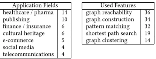
LDBC was founded by academia and industry in 2012 [7] in order to establish standard benchmarks for such new graph data management systems. LDBC has since developed a number of graph data management benchmarks [16, 20, 22] to contribute to more objective comparison among systems, informing prospective users of some of the strong- and weak-points of the various systems before even doing a Proof-Of-Concept study, while providing system engineers and architects clear targets for performance testing and improvement. LDBC regularly organizes Technical User Community (TUC) meetings, where not only members report on progress of LDBC task forces but also gather requirements and feedback from data practitioners, who are also present. There have been over 40 graph use-case presentations by data practitioners in these TUC meetings, who often are users of the graph data management software of LDBC members, such as IBM, Neo4j, Ontotext, Oracle and SAP. The topics and contents of these collected TUC presentations show that graph databases are being adopted over a wide range of application fields, as summarized in Figure 1. This further shows that the desired graph query language features are graph pattern matching (e.g., identification of communities in social networks), graph reachability (e.g., fraud detection in financial transactions or insurance), weighted path finding (e.g., route optimization in logistics, or bottleneck detection in telecommunications), graph construction (e.g., data integration in Bioinformatics or specialized publishing domains such as legal) and graph clustering (e.g., on social networks for customer relationship management).

1.1 Three Main Challenges

The following issues are observed about existing graph query languages. These observations are based on the LDBC TUC use-case analysis and feedback from industry practitioners:

Composability. The ability to plug and play is an essential step in standardization. Having the ability to plug outputs and inputs in a query language incentivizes its adoption (modularity, interoperability); simplify abstractions, users do not have to think about multiple data models during the query process; and increases its productivity, by facilitating

Application Fields Used Features

healthcare / pharma 14 graph reachability 36

publishing 10 graph construction 34

finance / insurance 6 pattern matching 32

cultural heritage 6 shortest path search 19

e-commerce 5 graph clustering 14

social media 4

telecommunications 4

Fig. 1. Graph database usage characteristics derived from the use-case presentations in LDBC TUC Meetings 2012-2017 (source: https://github.com/ldbc/tuc_presentations).

reuse and decomposition of queries. Current query languages do not provide full composability because they output tables of values, nodes or edges.

Path as first-class citizens. The notion of Path is fundamental for graph databases, because it introduces an interme-diate abstraction level that allows to represents how elements in a graph are related. The facilities provided by a graph query language to manipulate paths (i.e. describe, search, filter, count, annotate, return, etc.) increase the expressivity of the language. Particularly, the ability to return paths enables the user to post-process paths within the query language rather that in an ad-hoc manner [15].

Capture the core of available languages. Both the desirability of astandardquery language and the difficulty of achieving this, is well-established. This is particularly true for graph data languages due to the diversity of models and the rich properties of the graph model. This motivates our approach to take the successful functionalities of current languages as a base from where to develop the next generation of languages.

1.2 Contributions

Since the lack of a common graph query language kept coming up in LDBC benchmark discussions, it was decided in 2014 to create a task force to work on a common direction for property graph query languages. The authors are members of this task-force.

This paper presents G-CORE, a closed query language on Property Graphs. It is a coherent, comprehensive and consistent integration of industry desiderata and the leading functionalities found in industry practices and theoretical research.

The paper presents the following contributions:

Path Property Graph model. G-CORE treats paths as first-class citizens. This means that paths are outputs of certain queries. The fact that the language must be closed implies that paths must be part of the graph data model. This leads to a principled change of the data model:it extends property graphs with paths. That is, in a graph, there is also a (possibly empty) collection of paths; where a path is a concatenation of existing, adjacent, edges. Further, given that nodes, edges and paths are all first-class citizens, paths have identity and can also have labels and⟨property,value⟩pairs associated with them. This extended property graph model, called the Path Property Graph model, is backwards-compatible with the property graph model.

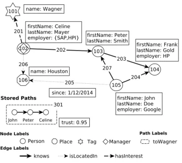
Fig. 2. A small social network. A Path Property Graph (PPG) is a Property Graph that can have “Stored Paths”.

Syntax and Semantics of G-CORE. A key contribution is the formal definition of G-CORE. This formal definition pre-vents any ambiguity about the functionality of the language, thus enabling the development of correct implementations. In particular, an open source grammar for G-CORE is available1.

Complexity results. To ensure that the query language is practically usable on large data, the design of G-CORE was built on previous complexity results. Features were carefully restricted in such ways that G-CORE is tractable (each query in the language can be evaluated efficiently). Thus, G-CORE provides the most powerful path query functionalities proposed so far, while carefully avoiding intractable complexity.

Organization of the paper. This paper first defines the Extended Property Graph model in Section 2. Then it explains G-CORE in Section 3 via a guided tour, using examples on the LDBC Social Network Benchmark dataset [16], which demonstrate its main features. We summarize our formal contributions, comprising syntax, semantics and complexity analysis of G-CORE in Section 4, while the details of these are described in Appendix A. In Section 5, we show how G-CORE can be easily extended to handle tabular data. We discuss related work in Section 6, before concluding in Section 7.

2 PATH PROPERTY GRAPHS

We first define the data model of G-CORE, which is an extension of the Property Graph data model [6, 25, 27, 35, 44]. We call this model thePath Property Graphmodel, or PPG model for short. LetLbe an infinite set of label names for nodes, edges and paths,Kan infinite set of property names, andVan infinite set of literals (actual values such as integer 1_{https://github.com/ldbc/ldbc_gcore_parser}

and real numbers, strings, dates, truth values⊥and⊤, that represent true and false, respectively, etc.). Moreover, given a setX, let FSET(X)denote the set of all finite subsets ofX (including the empty set), and FLIST(X)denote the set of all finite lists of elements fromX(including the empty list).

Definition 2.1. A PPG is a tupleG=(N,E,P,ρ,δ,λ,σ), where:

(1) Nis a finite set of node identifiers,Eis a finite set of edge identifiers andPis a finite set of path identifiers, whereN,EandPare pairwise disjoint.

(2) ρ:E→ (N×N)is a total function.

(3)δ :P→FLIST(N∪E)is a total function such that for everyp∈P, it holds thatδ(p)=[a₁,e₁,a₂, . . . ,a_n,e_n,a_n+1], where: (i)n ≥0, (ii)ej ∈Efor everyj ∈ {1, . . . ,n}, and (iii)ρ(e_j) =(a_j,a_j+1)orρ(ej) =(a_j+1,aj)for every

j∈ {1, . . . ,n}

(4) λ:(N∪E∪P) →FSET(L)is a total function.

(5)σ :(N∪E∪P)×K→FSET(V)is a total function for which there exists a finite set of tuples(x,k) ∈ (N∪E∪P)×K

such thatσ(x,k)_,∅

Given an edgeein a PPGG, ifρ(e)=(a,b), thenais the starting node ofeandbis the ending node ofe. The function

ρallows us to have several edges between the same pairs of nodes. Functionδassigns to each path identifierp∈Pan actualpathinG: this is a list[a₁,e₁,a₂, . . . ,a_n,e_n,a_n+1]satisfying condition (3) in Definition 2.1. Functionλis used to specify the set of labels of each node, edge, and path, while functionσis used to specify the values of a property for every node, edge, and path. To be precise, ifx ∈ (N∪E∪P)andk∈Kis a property name, thenσ(x,k)is the set of values of the propertykfor the identifierx. Observe that ifσ(x,k)=∅, then we implicitly assume that propertykis not defined for identifierx, as there is no value of this property for this object. Note that althoughKis an infinite set of property names, inGonly a finite number of properties are assigned values as we assume that there exists a finite set of tuples(x,k) ∈ (N∪E∪P) ×Ksuch thatσ(x,k)_,∅.

Example 2.2. As a simple example of a PPG, consider the small social network graph given in Figure 2. Here we have

N = {101,102,103,104,105,106},

E = {201,202,203,204,205,206,207},and

P = {301}

as node, edge, and path identifiers, respectively;

ρ = {2017→ (102,101), . . . ,2077→ (105,103)}and

δ = {3017→ [105,207,103,202,102]}

as edge and path assignments, respectively; and,

λ = {101 7→ {Tag},102 7→ {Person,Manager}, . . . ,201 7→ {hasInterest}, . . . ,301 7→ {toWagner}} and

σ = {(101,name) 7→ {Wagner}, . . . ,(205,since) 7→ {1/12/2014}, . . . ,(301,trust) 7→ {0.95}} as label and property value assignments, respectively.

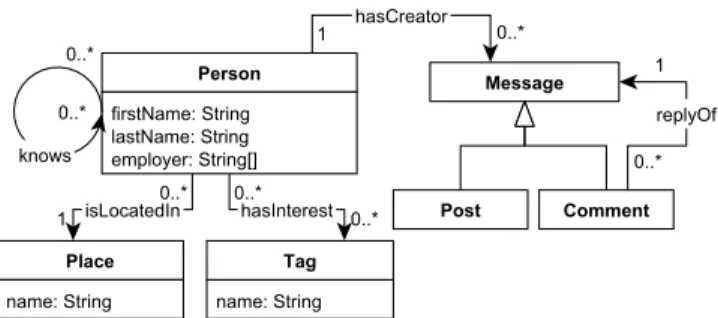
Fig. 3. Social Network Benchmark schema (simplified).

Paths. It is worth remarking that paths are included as a first-class citizens in this data model (at the level of nodes and edges). In particular, paths can have labels and properties, where the latter can be used to describe built-in properties like the length of the path. In our example above, the path with identifier 301 has label “toWagner” and value 0.95 on property “trust”.

For convenience, we usenodes(p)andedges(p)to denote the list of all nodes and edges of a path bound to a variable

p, respectively. Formally, ifδ(p)=[a₁,e₁,a₂, . . . ,e_n,a_n+1]thennodes(p)=[a₁, . . . ,a_n+1]andedges(p)=[e₁, . . . ,e_n]. In our example above,nodes(₃₀₁)=[102,103,₁₀₅]_andedges(₃₀₁)=[202,₂₀₇]_.

3 A GUIDED TOUR OF G-CORE

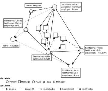
We will now demonstrate and explain the main features of the G-CORE language. The concrete setting is the LDBC Social Network Benchmark (SNB), as illustrated in the simple social network from Figure 2, whose (simplified) schema is depicted in Figure 3. Figure 4 depicts the toy instance (which we refer to associal_graph) on which our example queries are evaluated. The use-cases in these examples are data integration and expert finding in a social network.

Always returning a graph. Let us start with what is possibly one of the simplest G-CORE queries:

1 C O N S T R U C T (n) 2 MATCH (n:P e r s o n) 3 ON s o c i a l _ g r a p h

4 WHERE n.e m p l o y e r = ' Acme '

In G-CORE every query returns a graph, as embodied by theCONSTRUCTclause which is at the start of every query body. This example query constructs a new graph with no edges and only nodes, namely those persons who work at Acme – all the labels and properties that these person nodes had insocial_graphare preserved in the returned result graph.

Match and Filter. TheMATCH..ON..WHEREclause matches one or more (comma separated)graph patternson a named graph, using the homomorphic semantics [6].

Systems may omitONif there is adefaultgraph – let us assume in the sequel thatsocial_graphis the default graph. Parenthesis demarcate a node, wherenis a variable bound to the identity of a node,:Persona label, andn.employera property. The G-CORE builds on the ASCII-art syntax from Cypher [17] and the regular path expression syntax from PGQL [43], which has proven intuitive, effective and popular among property graph database users.

Fig. 4. Initial graph database (social_graph). Note that theknowsedges are drawn bi-directionally – this means there are two edges: one in each direction.

The previous example contains aWHEREfilter with the obvious semantics: it eliminates all matches where the employer is not Acme.

Multi-Graph Queries and Joins. A more useful query would be a simpledata integrationquery, where we might

have loaded (unconnected) company nodes into a temporary graphcompany_graph, but now want to create a unified graph where employees and companies are connected with an edge labeledworksAt. Let us assume thatcompany_graph contains nodes for Acme, HAL, CWI and MIT. As an aside, the real SNB dataset already contains such Company nodes with:worksAtedges to the employees (which in reality do not have anemployerproperty).

The below query has aMATCHclause with two graph patterns, matching these on two different input graphs. Graph patterns that do not have variables in common lead to the Cartesian product of variable bindings, but this query also has aWHEREclause that turns it into an equi-join:

5 C O N S T R U C T (c) < -[:w o r k s A t] -(n)

6 MATCH (c:C o m p a n y) ON c o m p a n y _ g r a p h, 7 (n:P e r s o n) ON s o c i a l _ g r a p h

8 WHERE c.name = n.e m p l o y e r

9 UNION s o c i a l _ g r a p h

TheUNIONoperator takes it intuitive meaning, and will be touched upon later when we talk about node and edge identity.

Generally speaking,MATCHproduces aset of bindingswhich alternatively may be viewed as a table having a column

for each variable and one row for each binding. Bindings typically contain node, edge and path identities, whose shape is opaque, but we use intuitive names prefixed # here:

c n #Acme #Alice #HAL #Celine #Acme #John

Dealing with Multi-Valued properties. In the previous query there is the complication thatn.employerismulti-valued for Frank Gold: he works for both MIT and CWI. Therefore, his person node fails to match with both companies. To explain this, we show the bindings and values ofc.nameandn.employerifWHERE c.name= n.employerwere omitted, and the query would be a Cartesian product:

c c.name n n.employer #MIT "MIT" #Peter

#CWI "CWI" #Peter #Acme "Acme" #Peter #HAL "HAL" #Peter

#MIT "MIT" #Frank {"CWI", "MIT"} #CWI "CWI" #Frank {"CWI", "MIT"} #Acme "Acme" #Frank {"CWI", "MIT"} #HAL "HAL" #Frank {"CWI", "MIT"} #MIT "MIT" #Alice "Acme" #CWI "CWI" #Alice "Acme" #Acme "Acme" #Alice "Acme" #HAL "HAL" #Alice "Acme" #MIT "MIT" #Celine "HAL" #CWI "CWI" #Celine "HAL" #Acme "Acme" #Celine "HAL" #HAL "HAL" #Celine "HAL" #MIT "MIT" #John "Acme" #CWI "CWI" #John "Acme" #Acme "Acme" #John "Acme" #HAL "HAL" #John "Acme"

Notice that according to the definition of our data model, the value ofc.nameis a set. But in the casec.nameis a singleton set, we omit curly braces, so we simply write"MIT"instead of{"MIT"}. In the table above, the rows in bold would be the ones that earlier led to bindings surviving the join. Essentially,"MIT"={"CWI","MIT"}and"CWI"={"CWI","MIT"}

evaluate toFALSE.

Note that Peter is unemployed, so hisn.employervalue is unbound. More precisely, its Person node does not have an employer property at all. In case of an absent property, its evaluation results in the empty set, which a length test can detect. G-CORE providesCASEexpressions to coalesce such missing data into other values.

One way to resolve the failing join for Frank, would be to useINinstead of=, so the comparisons mentioned earlier

resolve toTRUE: 10 C O N S T R U C T (c) < -[:w o r k s A t] -(n) 11 MATCH (c:C o m p a n y) ON c o m p a n y _ g r a p h, 12 (n:P e r s o n) ON s o c i a l _ g r a p h 13 WHERE c.name IN n.e m p l o y e r 14 UNION s o c i a l _ g r a p h

Notice that theINoperator can be used whenc.nameis a singleton set, as in this case it is natural to ask whether the value inc.nameis an element ofn.employer. If we need to comparec.namewithn.employeras sets, then the operatorSUBSET

can be used.

Another way to deal with this in G-CORE is to bind a variable ({name:e}) to theemployerproperty, which unrolls multi-valued properties into individual bindings:

15 C O N S T R U C T (c) < -[:w o r k s A t] -(n) Manuscript submitted to ACM

16 MATCH (c:C o m p a n y) ON c o m p a n y _ g r a p h, 17 (n:P e r s o n {e m p l o y e r=e}) ON s o c i a l _ g r a p h

18 WHERE c.name = e

19 UNION s o c i a l _ g r a p h

Inside theMATCHexpression that binds a node, curly braces can be used to bind variables to property values. The set

of bindings for thisMATCH(which includes the join) now has three variables and the following bindings:

c n e

#MIT #Frank "MIT" #CWI #Frank "CWI" #Acme #Alice "Acme" #HAL #Celine "HAL" #Acme #John "Acme"

Construction that respects identities. TheCONSTRUCToperation fills a graph pattern (used as template) for each binding in the set of bindings produced by theMATCHclause. Edges are denoted with square brackets, and can be pointed towards either direction; in this case there is no edge variable, but there is an edge label:worksAt. Note, to be precise,

thatCONSTRUCTby defaultgroupsbindings when creating elements. Nodes are grouped by node identity, and edges by the combination of source and destination node. While five new edges are created here, they are between four existing persons and four existing companies due to this grouping. For instance, the person#Frank, who works for both MIT and CWI, gets two:worksAtedges, to respectively company#MITand company#CWI.

In the last line of this example query, weUNION-ed these new edges with the original graph, resulting in an enriched graph: the original graph plus five edges. The “full graph” query operators like union and difference are defined in terms of node, edge and path identities. These identities are taken from the input graph(s) of the query. G-CORE is a query language, not an update language. Even thoughCONSTRUCTallows withSETprop:=valandREMOVEpropto change properties and values (a later example will demonstrateSET), this does not modify the graph database, it just changes the result of that particular query. The practice of returning a graph that shares (parts of) nodes, edges and paths with its inputs, using this concept of identity, provides opportunities for systems to share memory and storage resources between query inputs and outputs.

A shorthand form for the union operation is to include a graph name directly in the comma separated list ofCONSTRUCT

patterns, as depicted in the next query:

20 C O N S T R U C T s o c i a l _ g r a p h,

21 (x GROUP e :C o m p a n y {name:=e}) < -[y:w o r k s A t] -(n) 22 MATCH (n:P e r s o n {e m p l o y e r=e})

Graph Aggregation. The above query demonstratesgraph aggregation. Supposing there would not have been any

company nodes in the graph, we might also have created them with this excerpt:

CONSTRUCT(n)-[y:worksAt]->(x:Company{name:=n.employer})

However, this unbound destination nodexwould create a company node foreachbinding2. This is not what we want: we want only one company per unique name. Graph aggregation therefore allows an explicitGROUPclause in each graph

pattern element. Thus, in the above query withGROUP e, we create only one company node for each unique value ofe in the binding set. Here the curly brace notation is used insideCONSTRUCTto instantiate theCompany.nameproperty in the newly created nodes.

2_{In addition, it would create a company with thename property with the values{"CWI","MIT"}.}

The set of bindings of our graph aggregation query example has the same variablesnandevariables of the previous binding set. TheCONSTRUCTfor node expression(n)groups by node identity so instantiates the nodes with identity#Frank, #Alice,#Celineand#Johnin the query result. These nodes were already part ofsocial_graph, so given that theCONSTRUCTis UNION-ed with that, no extra nodes result.

For the(xGROUP e..)node expression,CONSTRUCTgroups byeinto bindings"CWI","MIT","Acme", and"HAL"and becausex is unbound, it will create four new nodes with, say, identities#CWI,#MIT,#Acmeand#HAL. For the edges to be constructed, G-CORE performs by default grouping of the bindings on the combination of source and destination node, and this results in again five new edges.

When using bound variables in aCONSTRUCT, they must be of the right sort: it would be illegal to usen(a node) in the place ofy(an edge) here. In case anedgevariable (here:y) would have been bound (in theMATCH),CONSTRUCTimposes the restriction that its node variables must also be bound, and be bound to exactly its source and destination nodes, because changing the source and destination of an edge violates its identity. However, it can be useful to bind edges inMATCH

and use these to construct edges with a new identity, which are copies of these existing edges in terms of labels and property-values. For this purpose, G-CORE supports the-[=y]-syntax which makes a copy of the boundyedges (as well as the(=n)syntax for nodes). Then, the above restriction does not apply. With the copy syntax, it is even possible to copy all labels and properties of a node to an edge (or a path) and vice versa.

In this example,xandywere unbound and could have been omitted. In the preceding examples, they were in fact omitted. Unbound variables in aCONSTRUCTare useful if they occurmultipletimes in the construct patterns, in order

to ensure that the same identities will be used (i.e., to connect newly created graph elements, rather than generate independent nodes and edges).

Storing Paths with @p. G-CORE is unique in its treatment of paths, namely as first-class citizens. The below query demonstrates finding the three shortest paths from John Doe towards each other person who lives at his location, reachable overknowsedges, using Kleene star notation<:knows*>:

23 C O N S T R U C T (n) -/@p:l o c a l P e o p l e{d i s t a n c e:=c}/ - >(m) 24 MATCH (n) -/3 S H O R T E S T p<:kn ows* > COST c/ - >(m) 25 WHERE (n:P e r s o n) AND (m:P e r s o n)

26 AND n.f i r s t N a m e = ' John ' AND n.l a s t N a m e = ' Doe ' 27 AND (n) -[:i s L o c a t e d I n] - >() < -[:i s L o c a t e d I n] -(m)

In G-CORE, paths are demarcated with slashes-/ /-. In the above examplep <:knows*>binds the shortest path between

the single noden(i.e. John Doe) and every possible personm, under the restriction that this target person lives in the same place. By writing e.g.,-/3SHORTESTp <:knows*>/->we obtain multiple shortest paths (at most 3, in this case)

for every source–destination combination; if the number 3 would be omitted, it would default to 1. In case there are multiple shortest paths with equal cost between two nodes, G-CORE delivers just any one of them. By writing

p <:knows*> COSTc/->we bind the shortest path cost to variablec. By default, the cost of a path is its hop-count (length).

We will define weighted shortest paths later. If we would not be interested in the length,COSTccould be omitted. InCONSTRUCT(n)-/@p:localPeople{distance:c}, we see the bound path variable@p. The@prefix indicates astored path, that is, this query is delivering a graph with paths. Each path is stored attaching the label:localPeople, and its cost as propertydistance.

The graph returned by this query – which lacks aUNIONwith the originalsocial_graph– is aprojectionof all nodes and edges involved in these stored paths. We omitted a figure of this for brevity.

Fig. 5. Graph viewsocial_graph1, which addsnr_messageproperties to the originalsocial_graph(social_graph2issocial_graph1plus the Stored Paths in the grey box).

Reachability and All Paths. In a similar query where we just returnm, and do not store paths, the<:knows*>path

expression semantics is areachabilitytest:

28 C O N S T R U C T (m)

29 MATCH (n:P e r s o n) -/ <:k now s* >/ - >(m:P e r s o n)

30 WHERE n.f i r s t N a m e = ' John ' AND n.l a s t N a m e = ' Doe ' 31 AND (n) -[:i s L o c a t e d I n] - >() < -[:i s L o c a t e d I n] -(m)

In this case we use-/<:knows*>/->without theSHORTESTkeyword. UsingALLinstead ofSHORTEST: asking forallpaths, is not allowed if a path variable is bound to it and used somehwere, as this would be intractable or impossible due to an infinite amount of results. However, G-CORE can support it in the case where the path variable is only used to return a graph projection of all paths:

32 C O N S T R U C T (n) -/p/ - >(m)

33 MATCH (n:P e r s o n) -/ALL p<:kn ows* >/ - >(m:P e r s o n) 34 WHERE n.f i r s t N a m e = ' John ' AND n.l a s t N a m e = ' Doe ' 35 AND (n) -[:i s L o c a t e d I n] - >() < -[:i s L o c a t e d I n] -(m)

The method [10] shows how the materialization of all paths can be avoided by summarizing these paths in a graph projection; hence this functionality is tractable.

Existential Subqueries. In the SNB graph,isLocatedInis not a simple string attribute, but an edge to a city, and the three previous query examples used pattern matching directly in theWHEREclause:(n)-[:isLocatedIn]->()<-[:isLocatedIn]-(m). G-CORE allows this and uses implicit existential quantification, which here is equivalent to:

36 WHERE E X I ST S ( 37 C O N S T R U C T ()

38 MATCH (n) -[:i s L o c a t e d I n] - >() < -[:i s L o c a t e d I n] -(m) )

This constructs one new node (unbound anonymous node variable()) for each match ofnandmcoinciding in the city where they are located – where that city is represented by a()again. Whenever such a subquery evaluates to the empty graph, the automatic existential semantics ofWHEREevaluates toFALSE; otherwise toTRUE.

Views and Optionals. The fact that G-CORE isclosedon the PPG data model means that subqueries and views are possible. In the following example we create such a view:

39 GRAPH VIEW s o c i a l _ g r a p h 1 AS ( 40 C O N S T R U C T s o c i a l _ g r a p h, 41 (n) -[e] - >(m) SET e.n r _ m e s s a g e s := COUNT(*) 42 MATCH (n) -[e:k now s] - >(m) 43 WHERE (n:P e r s o n) AND (m:P e r s o n) 44 O P T I O N A L (n) < -[c1] -(msg1:Post|C o m m e n t) , 45 (msg1) -[:r e p l y _ o f] -(msg2) , 46 (msg2:Post|C o m m e n t) -[c2] - >(m) 47 WHERE (c1:h a s _ c r e a t o r) AND (c2:h a s _ c r e a t o r) )

The result of this graph view can be seen in Figure 5. To each:knowsedge, this view adds anr_messagesproperty, using

theSET.. :=sub-clause. This sub-clause ofCONSTRUCTcan be used to modify properties of nodes, edges and paths that

are being constructed. This particularnr_messagesproperty contains the amount of messages that the two personsnand mhave actually exchanged, and is a reliable indicator of the intensity of the bond between two persons.

The edge construction(n)-[e]->(m)adds nothing new, but as described before, performs implicit graph aggregation,

where bindings are grouped onn,m,e, andCOUNT(*)evaluates to the amount of occurrences of each combination. This example also demonstratesOPTIONALmatches, such that people who know each other but never exchanged a message still get a propertye.nr_messages=0. All patterns separated by comma in anOPTIONALblock must match. Technically, the set of bindings from the mainMATCHis left outer-joined with the one coming out of theOPTIONALblock (and there may be more than oneOPTIONALblocks, in which case this repeats). There can be multipleOPTIONALblocks, and eachOPTIONAL

block can have its ownWHERE; we demonstrate this here by moving some label tests toWHEREclauses (on:Personand

:has_creator). This query also demonstrates the use of disjunctive label tests (msg1:Post|Comment).

If a query contains multipleOPTIONALblocks, they have to be evaluated from the top to the bottom. For example, to evaluate the following pattern:

48 MATCH (n:P e r s o n)

49 O P T I O N A L (n) -[:w o r k s A t] - >(c) 50 O P T I O N A L (n) -[:l i v e s I n] - >(a)

we need to perform the following steps: evaluate(n:Person)to generate a binding setT1, evaluate(n)-[:worksAt]->(c)to generate a binding setT2, compute the left-outer join ofT1withT2to generate a binding setT3, evaluate(n)-[:livesIn

]->(a)to generate a binding setT4, and compute the left-outer join ofT3withT4to generate a binding setTthat is the

result of evaluating the entire pattern. Obviously, in this case the order of evaluation is not relevant, and the previous pattern is equivalent to:

51 MATCH (n:P e r s o n)

52 O P T I O N A L (n) -[:l i v e s I n] - >(a) 53 O P T I O N A L (n) -[:w o r k s A t] - >(c)

However, the order of evaluation can be relevant if the optional blocks of a pattern shared some variables that are not mentioned in the first pattern. For example, in the following expression the variableais mentioned in the optional blocks but not in the first pattern(n:Person):

54 MATCH (n:P e r s o n)

55 O P T I O N A L (n) -[:w o r k s A t] - >(a) 56 O P T I O N A L (n) -[:l i v e s I n] - >(a)

Arguably, such a pattern is not natural, and it should not be allowed in practice. By imposing the simple syntactic restriction that variables shared by optional blocks have to be present in their enclosing pattern, one can ensure that the semantics of a pattern with multipleOPTIONALblocks is independent of the evaluation order [31].

Weighted Shortest Paths. The finale of this section describes an example ofexpert finding: let us suppose that John Doe wants to go to a Wagner Opera, but none of his friends likes Wagner. He thus wants to know which friend to ask to introduce him to a true Wagner lover who lives in his city (or to someone who can recursively introduce him). To optimize his chances for success, he prefers to try “friends” who actually communicate with each other. Therefore we look for theweightedshortest path over thewKnows(“weighted knows”)path patterntowards people who like Wagner, where the weight is the inverse of the number of messages exchanged: the more messages exchanged, the lower the cost (though we add one to the divisor to avoid overflow). For each Wagner lover, we want a shortest path.

In G-CORE, weighted shortest paths are specified overbasic path patterns, defined by aPATH ..WHERE ..COSTclause, because this allows to specify a cost value for each traversed path pattern. The specified cost must be numerical, and larger than zero (otherwise a run-time error will be raised), where the full cost of a path (to be minimized) is the sum of the costs of all path segments. If theCOSTis omitted, it defaults to 1 (hop count).

57 GRAPH VIEW s o c i a l _ g r a p h 2 AS ( 58 PATH w K n o w s = (x) -[e:kno ws] - >(y) 59 WHERE NOT ' Acme ' IN y.e m p l o y e r

60 COST 1 / (1 + e.n r _ m e s s a g e s)

61 C O N S T R U C T s o c i a l _ g r a p h 1, (n) -/@p:t o W a g n e r/ - >(m) 62 MATCH (n:P e r s o n) -/p<~w K n o w s* >/ - >(m:P e r s o n) 63 ON s o c i a l _ g r a p h 1

64 WHERE (m) -[:h a s I n t e r e s t] - >(:Tag {name= ' W a g n e r ' }) 65 AND (n) -[:i s L o c a t e d I n] - >() < -[:i s L o c a t e d I n] -(m) 66 AND n.f i r s t N a m e = ' John ' AND n.l a s t N a m e = ' Doe ' )

The result of this graph view (social_graph2) was already depicted in Figure 5: it adds tosocial_graph1two stored paths. Apart fromGRAPH VIEW nameAS (query), and similar to CREATE VIEW in SQL which introduces a global name for a query expression, G-CORE also supports aGRAPH nameAS (query1)query2clause which, similar to WITH in SQL, introduces a name that is only visible insidequery2.

Powerful Path Patterns. BasicPATHpatterns are a powerful building block that allow complex path expressions as

concatenations of these patterns [43] using a Kleene star, yet still allow for fast Dijkstra-based evaluation. In G-CORE, these path patterns can even be non-linear shapes, asPATHcan take a comma-separated list of multiple graph patterns.

But, the path pattern must contain a start and end node (apath segment), which is taken to be the first and last node in its first graph pattern. This ensures path patterns can be stitched together to form paths – a path pattern always contains a path segment between its start and end nodes. These basic path patterns can also containWHEREconditions,

Matching

Matching all patterns (Homomorphism) *

Matching literal values 18, 22

Matchingkshortest paths 24

Matching all shortest paths 29 Matching weighted shortest paths 60 (multi-segment) optional matching 44

Querying

Querying multiple graphs 6

Queries on paths 69

Filtering matches 4,8,13,18,26,30,34,59,64,71 Filtering path expressions 58

Value joins 8

Cartesian product 11

List membership 13

Subqueries

Set operations on graphs 8, 14, 19 Existential subqueries - Implicit 27, 31, 35 - Explicit 36 Construction Graph construction * Graph aggregation 21 Graph projection 23 Graph views 39, 57 Property addition 41

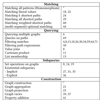
Table 1. Overview ofG-COREfeatures and their line occurrences in the example queries in Section 3.

without restrictions on their complexity. As John Doe wants his preference for Wagner to remain unknown at his work, we exclude employees of Acme from occurring on the path3. The result of this query is a viewsocial_graph2in which all these shortest paths from John Doe to Wagner lovers have been materialized (the@pin(n)-/@p:toWagner/->(m)).

A unique capability of G-CORE is to query and analyze databases of potentially many stored paths. We demonstrate this in the final query, where we score John’s friends for their aptitude:

67 C O N S T R U C T (n) -[e:w a g n e r F r i e n d {sco re:=COUNT(*) }] - >(m) 68 WHEN e.s cor e > 0

69 MATCH (n:P e r s o n) -/@p:t o W a g n e r/ - >() , (m:P e r s o n) 70 ON s o c i a l _ g r a p h 2

71 WHERE n = n ode s(p) [1]

For the:toWagnerpaths, we usenodes(p)[1]to look at the second node in each path, i.e. a direct friend of John Doe.

G-CORE starts counting at 0 sonodes(my_path)[n]returns then−1 item from the list returned by the functionnodes(), which returns all nodes on a path. For these direct friends we count how often they occur as the start of:toWagnerpaths. These scores has been attached as ascoreproperty to new:wagnerFriendedges. Since in the toy example there are only two Wagner lovers and thus two shortest paths to them, both via Peter, the result of this query is a single:wagnerFriend edge between John and Peter with score 2.

3_{Note that non-linear path patterns, such asPATH(a)-[]-(b),(b)-(c)add power over linear patterns with existential filters:PATH(a)-[]-(b)WHERE}

(b)-(c), because the latter cannot bind variables. In G-CORE, variableccan be used in aCOSTexpression. Manuscript submitted to ACM

4 FORMALIZING AND ANALYZING G-CORE

One of the main goals of this paper is to provide a formal definition of the syntax and semantics of a graph query language including the features shown in the previous sections. Formally, a G-CORE query is defined by the following top-down grammar:

query::=headClause fullGraphQuery

headClause::=ε | pathClause headClause | graphClause headClause fullGraphQuery::=basicGraphQuery |

(_{fullGraphQuery setOp fullGraphQuery}) setOp::=Union | Intersect | Minus basicGraphQuery::=constructClause matchClause

Thus, a G-CORE query consists of a sequence of Path and Graph clauses, followed by a full graph query, i.e., a combination of basic graph queries under the set operations of union, intersection and difference. A basic graph query consists of a single Construct clause followed by one Match clause. We have seen examples of all these features in Section 3.

In Appendix A, we provide formal definitions of the syntax and semantics of G-CORE. The basic idea of the language is, given a PPGG, to create a new PPGHusing the Construct clause. This is achieved, in turn, by applying an intermediate step provided by the Match clause. The application of such a clause creates a set of bindingsΩ, based on a graph pattern that is evaluated overG. The interaction between the Match and the Construct clause is explained in more detail below:

• The result of evaluating the graph patternφthat defines the content of a Match clause over a PPGGalways corresponds to a setΩof bindings, which is denoted byJφKG. The bindings inΩcan then be filtered by using boolean conditions specified in the Where clause.

• A Construct clauseψthen takes as input both the PPGGand the set of bindingsΩ, and produces a new PPG

H, which is denoted byJψKΩ,G. Note thatGis also an input in the evaluation ofψ, as the set of bindingsΩcan make reference to objects whose labels and properties are defined inG.

The role of the Path clause is to define complex path expressions, as well as the cost associated with them, that can in turn be used in graph patterns in the Match clause. In this way, it is possible to define rich navigational patterns on graphs that capture expressive query languages that have been studied in depth in the theoretical community (e.g., the class ofregular queries[34]).

Complexity analysis. The G-CORE query language has been carefully designed to ensure that G-CORE queries can

be evaluated efficiently indata complexity. Formally, this means that for each fixed G-CORE queryq, the resultJqKGof evaluatingqover an input PPGGcan be computed in polynomial time. The main reasons that explain this fact are given below.

First of all, graph patterns correspond (essentially) to conjunctions of atoms expressing that two nodes are linked by a path satisfying a certain regular expression over the alphabet of node and edge labels. The setΩof all bindings of a fixed graph patternφover the input PPGGcan then be easily computed in polynomial time: we simply look for all possible ways of replacing node and edge variables inφby node and edge identifiers inG, respectively, and then for

each path variableπrepresenting a path inGfrom nodeuto nodevwhose label must conform to a regular expressionr, we replaceπby the shortest/cheapest path inGfromutovthat satisfiesr(if it exists). This can be done in polynomial time by applying standard automata-theoretic techniques in conjunction with Dijkstra-style algorithms. (Notice that the latter would not be true if our semantics was based on simple paths; in fact, checking if there is a simple path in an extended property graph whose label satisfies a fixed regular expression is an NP-complete problem [23]).

Suppose, now, that we are given a fixed G-CORE queryqthat corresponds to a sequence of clauses followed by a full graph queryq′. Each clause is defined by a graph patternφwhose evaluation corresponds to a binary relation over the nodes of the input PPGG. By construction, the graph patternφmight mention binary patterns which are defined in previous clauses. Therefore, it is possible to iteratively evaluate in polynomial time all graph patternsφ1, . . . ,φkthat are mentioned in the clauses ofq. Once this process is finished, we proceed to evaluateq′(which is defined in terms of theφi’s).

By definition,q′is a boolean combination of full graph queriesq1, . . . ,qm. It is thus sufficient to explain how to

evaluate each such a full graph queryqj in polynomial time. We can assume by construction thatqj consists of a Construct clause applied over a Match clause. We first explain how the set of bindings that satisfy the Match clause can be computed in polynomial time. Since one or more Optional clauses could be applied over the Match clause, the semantics is based on the setΩofmaximalbindings for the whole expression, i.e., those that satisfy the primary graph pattern expressed in the Match clause, and as many atoms as possible from the basic graph patterns that define the Optional clauses. The computation ofΩcan be carried out in polynomial time by a straightforward extension of the aforementioned techniques for efficiently evaluating basic graph patterns. Finally, filteringΩin accordance with the boolean conditions expressed in the Where clause can easily be done in polynomial time (under the reasonable assumption that such conditions can be evaluated efficiently). Recall that a possible such a condition is ExistsQ, forQ a subquery. We then need to check whether the evaluation ofQoverGyields an empty graph. We inductively assume the existence of an efficient algorithm for checking this.

Finally, the application of the Construct clause on topGand the setΩof bindings generated by the Match clause can be carried out in polynomial time. Intuitively, this is because the operations allowed in the Construct clause are defined by applying some simple aggregation and grouping functions on top of bindings generated by relational algebra operations.

Given that all evaluation steps of G-CORE have polynomial complexity in data size, we conclude that G-CORE is tractable.

5 EXTENSIONS OFG-CORE

Practical use of graphs often requires handling tabular data. This suggests that extending G-CORE with additional functionality for projecting tabular results or constructing graphs from imported tabular data may be useful.

Projecting tabular results. In order to integrate the results of graph matching into another system, it would be necessary or at least convenient to be able to produce a tabular projection from a query. It is quite straightforward to imagine the set of bindings produced byMATCHas a table, and use that to return a tabular projection. To achieve this,

G-CORE could be extended with aSELECTclause for projecting expressions into a table. Such a tabular projection clause would also allow the introduction of other common relational operations for slicing, sorting, and aggregation, similar to Cypher’sRETURNclause or theSELECTclauses of SQL or SPARQL. Furthermore,SELECTcould be used for adding various forms of expression-level subqueries, such as scalar subqueries or list subqueries.

Consider this example of a query that uses tabular projection:

72 S E L E C T m.l a s t N a m e + ' , ' + m.f i r s t N a m e AS f r i e n d N a m e

73 MATCH (n:P e r s o n) -/ <:k no ws* >/ - >(m:P e r s o n)

74 WHERE n.f i r s t N a m e = ' John ' AND n.l a s t N a m e = ' Doe ' 75 AND (n) -[:i s L o c a t e d I n] - >() < -[:i s L o c a t e d I n] -(m)

This query matches persons with the name “John Doe” together with indirect friends that live in the same city and returns a table with the names of these friends.

It should be noted that the introduction of tabular projection into G-CORE changes the language to a multi-sorted language that is capable of either producing a table or a graph. Such a language would no longer be fully closed under graphs in a strict sense, which is one reason why this extension has been left to the future.

Importing tabular data. Conversely, integration of G-CORE with existing systems raises the question of how pre-existing tabular data could be processed in a pure graph query language. Next we present two different alternative proposals for how tabular data could be brought in to the graph world of G-CORE.

Binding table inputs. One way to import tabular data would be through the introduction of a newFROM<table>clause that would import sets of scalar bindings from a table, which could be used for defining a graph using theCONSTRUCT

clause such as in this example:

76 C O N S T R U C T

77 (cust GROUP c u s t N a m e :C u s t o m e r {name:=c u s t N a m e}) , 78 (prod GROUP p r o d C o d e :P r o d u c t {code:=p r o d C o d e}) , 79 (cust) -[:b o u g h t] - >(prod)

80 FROM o r d e r s

This will construct a new graph from an input table of customer namescustNameand product codesprodCodeby connecting per-customer and per-product nodes as given by the table.

Interpreting tables as graphs. Another alternative is to allow theMATCH.. ON ..to treat a tabular input followingON

as a graph consisting of only isolated nodes that correspond to each row in the table. The properties of these nodes are the columns of the table and the values are the fields of the corresponding row.

If we express the previous example using this syntax, it would now look as follows:

81 C O N S T R U C T

82 (cust GROUP o.c u s t N a m e :C u s t o m e r {name:=o.c u s t N a m e}) , 83 (prod GROUP o.p r o d C o d e :P r o d u c t {code:=o.p r o d C o d e}) , 84 (cust) -[:b o u g h t] - >(prod)

85 MATCH (o) ON o r d e r s

6 DISCUSSION AND RELATED WORK

Graph query languages have been extensively researched in the past decades, and comprehensive surveys are available. Angles and Gutierrez [8] surveyed GQLs proposed during the eighties and nineties, before the emergence of current (practical) graph database systems. Wood [45] studied GQLs focusing on their expressive power and computational complexity. Angles [5] compares graph database systems in terms of their support for essential graph queries. Barceló [11] studies the expressiveness and complexity of several navigational query languages. Recently, Angles et al. [6] presented

a study on fundamental graph querying functionalities (mainly graph patterns and navigational queries) and their implementation in modern graph query languages.

The extensive research on querying graph databases has not give rise yet to a standard query language for property graphs (like SQL for the relational model). Nevertheless, there are several industrial graph database products on the market. Gremlin [18] is a graph-based programming language for property graphs which makes extensive use of XPath to support complex graph traversals. Cypher [13], originally introduced by Neo4j and now implemented by a number of vendors, is a declarative query language for property graphs that has graph patterns and path queries as basic constructs. We primarily consider version 9 of Cypher as outlined by [17, 26], while recognizing that Cypher is an evolving language where several advancements compared to Cypher 9 have already been made. Oracle has developed PGQL [43], a graph query languages that is closely aligned to SQL and that supports powerful regular path expressions. Several implementations of PGQL, both for non-distributed [38] and distributed systems [36], exist. Here, we consider PGQL 1.1 [29], which is the most recent version that is commercially available [28].

G-CORE has been designed to support most of the main and relevant features provided by Cypher, PGQL, and Gremlin. Next we describe the main differences among G-CORE, Cypher, PGQL, and Gremlin based on the query features described in Section 3. Some features (e.g. aggregate operators) will not be discussed here as there are not substantial differences from one language to other.

Graph pattern queries. The notion of basic graph pattern, i.e. the conjunction of node-edge-node patterns with filter conditions over them, is intrinsically supported by Cypher, PGQL and G-CORE. Some differences arise regarding the support for complex graph patterns (i.e. union, difference, optional). Both Cypher and G-CORE define the UNION operator to merge the results of two graph patterns. The absence of graph patterns (negation) is mainly supported via existential subqueries. It is expressed in G-CORE, Cypher and PGQL with the WHERE NOT (EXISTS) clause. Optional graph patterns can be explicitly declared in G-CORE and Cypher with the OPTIONAL clause. PGQL does not support optional graph patterns, although they can be roughly simulated with length-restricted path expressions (see below). Although Gremlin is focused on navigational queries, it supports complex graph patterns (including branches and cycles) as the combination of traversal patterns.

Path queries. G-CORE, Cypher and PGQL support path queries in terms of regular path expressions (i.e. edges can be labeled with regular expressions). The main difference between Cypher 9 and PGQL is that the closure operator is restricted to a single repeated label / value. Both Cypher and PGQL support path length restrictions, a feature that although can be simulated using regular expressions, improves the succinctness of the language. Gremlin supports arbitrary or fixed iteration of any graph traversal (i.e. it is more expressive than regular path queries). Similar to Cypher, Gremlin allows specifying the number of times a traversal should be performed.

Query output. The general approach followed by Cypher 9 and PGQL is to return tables with atomic values (e.g. property values). This approach can be extended such that a result table can contain complex values. The extension in Cypher 9 allows returning nodes, edges, and paths. Recent implementations of Cypher have the ability to return graphs alongside this table [1, 32]. Gremlin also supports returning complete paths as results. In contrast, G-CORE has been designed to return graphs with paths as first class citizens.

Query composition. With the output of a query in G-CORE being a graph, it follows naturally that queries can be composed by querying the output of one query by means of another query. Neither Cypher 9, PGQL or SPARQL supports

this capability. Gremlin supports creating graphs and then populate them before querying the new graph. A notable parallel to G-CORE is the evolution of Cypher 10, where queries are composed through the means of “table-graphs”. Cypher 10 expresses queries with multiple graphs and a driving table as input, and produces a set of graphs along with a table as output. This allows Cypher 10 queries to compose both linearly and through correlated subqueries [17].

Evaluation semantics. There are several variations among the languages regarding the semantics for evaluating graph and path expressions. In the context of graph pattern matching semantics, G-CORE, PGQL, and Gremlin follow the homomorphism-based semantics (i.e. no restrictions are imposed during matching), and Cypher 9 follows a no-repeated-edge semantics (i.e. two variables cannot be bound to the same term in a given match) to prevent matching of potentially infinite result sets when enumerating all paths of a pattern. With respect to the evaluation of path expressions, G-CORE uses shortest-path semantics (i.e. paths of minimal length are returned), Cypher 9 implements no-repeated-edge semantics (i.e. each edge occurs at most once in the path), and Gremlin follows arbitrary path semantics (i.e. all paths are considered). Additionally, Cypher 9 and PGQL allow changing the default semantics by using built-in functions (e.g.allShortestPaths).

Expressive power versus efficiency. A balance between expressiveness and efficiency (complexity of evaluation) means a balance between practice and theory. Currently no industrial graph query language has a theoretical analysis of its complexity and, conversely, theoretical results have not been systematically translated into a design. One of the main virtues of G-CORE is that its design is the integration of both sources of knowledge and experience.

SPARQL and RDF. In this paper we concentrated on property graphs, but there are other data models and query

languages available. A well-known alternative is the Resource Description Framework (RDF), a W3C recommendation that defines a graph-based data model for describing and publishing Web metadata. RDF has a standard query language, SPARQL [33], which was designed to support several types of complex graph patterns (including union and optional). Its latest version, SPARQL 1.1 [19], adds support for negation, regular path queries (calledproperty paths), subqueries and aggregate operators. The path queries support reachability tests, but paths cannot be returned, nor can the cost of paths be computed. The evaluation of SPARQL graph patterns follows a homomorphism-based bag semantics, whereas property paths are evaluated using an arbitrary paths semantics [6]. SPARQL allows queries that return RDF graphs, however creating graphs consisting of multiple types of nodes (e.g., belonging to different RDF schema classes; having different properties) in one query is not possible as SPARQL lacks flexible graph aggregation: its CONSTRUCT directly instantiates a single binding table without reshaping. Such constructed RDF graphs can not be reused as subqueries, that is, for composing queries; nor does the language offer “full graph” operations to union or diff at the graph level. We think the ideas outlined in G-CORE could also inspire further development of SPARQL.

7 CONCLUSIONS

Graph databases have come of age. The number of systems, databases and query languages for graphs, both commercial and open source, indicates that these technologies are gaining wide acceptance [3, 4, 9, 12, 14, 21, 24, 25, 30, 37–42].

At this stage, it is relevant to begin making efforts towards interoperability of these systems. A language like G-CORE could work as a base for integrating the manifold models and approaches towards querying graphs.

We defend here two principles we think should be at the foundations of the future graph query languages: compos-ability, that is, having graphs and their mental model as departure and ending point and treat the most popular feature of graphs, namelypaths, as first class citizens.

The language we present, G-CORE, which builds on the experiences with working systems, as well as theoretical results, show these desiderata are not only possible, but computationally feasible and approachable for graph users. This paper is a call to action for the stakeholders driving the graph database industry.

REFERENCES

[1] 2017. Cypher for Apache Spark. (2017). https://github.com/opencypher/cypher-for-apache-spark [2] 2017. The openCypher Project. (2017). http://www.openCypher.org

[3] AgensGraph - The Performance-Driven Graph Database. 2017. (2017). http://www.agensgraph.com/ [4] Amazon Neptune - Fast, reliable graph database build for cloud. 2017. (2017). https://aws.amazon.com/neptune/

[5] Renzo Angles. 2012. A comparison of current graph database models. In4rd Int. Workshop on Graph Data Management: Techniques and Applications. [6] Renzo Angles, Marcelo Arenas, Pablo Barceló, Aidan Hogan, Juan L. Reutter, and Domagoj Vrgoc. 2017. Foundations of Modern Query Languages

for Graph Databases.Comput. Surveys50, 5 (2017). https://doi.org/10.1145/3104031

[7] Renzo Angles, Peter Boncz, Josep Larriba-Pey, Irini Fundulaki, Thomas Neumann, Orri Erling, Peter Neubauer, Norbert Martinez-Bazan, Venelin Kotsev, and Ioan Toma. 2014. The Linked Data Benchmark Council: A Graph and RDF Industry Benchmarking Effort.SIGMOD Record43, 1 (May 2014), 27–31.

[8] Renzo Angles and Claudio Gutierrez. 2008. Survey of graph database models.ACM Computing Surveys (CSUR)40, 1 (2008), 1–39. [9] ArangoDB - Native multimodel database. 2017. (2017). https://arangodb.com/

[10] Pablo Barceló, Leonid Libkin, Anthony W. Lin, and Peter T. Wood. 2012. Expressive Languages for Path Queries over Graph-Structured Data.TODS

37, 4, Article 31 (Dec. 2012), 46 pages.

[11] Pablo Barceló Baeza. 2013. Querying graph databases. InProc. of the 32nd Symposium on Principles of Database Systems (PODS). ACM, 175–188. [12] Blazegraph. 2017. (2017). https://www.blazegraph.com/

[13] Cypher - Graph Query Language. 2017. (2017). http://neo4j.com/developer/cypher-query-language/ [14] DataStax Enterprise Graph. 2017. (2017). https://www.datastax.com/products/datastax-enterprise-graph

[15] Anton Dries, Siegfried Nijssen, and Luc De Raedt. 2009. A Query Language for Analyzing Networks. InProc. of the 18th ACM Conference on

Information and Knowledge Management (CIKM). ACM, 485–494.

[16] Orri Erling, Alex Averbuch, Josep Larriba-Pey, Hassan Chafi, Andrey Gubichev, Arnau Prat, Minh-Duc Pham, and Peter Boncz. 2015. The LDBC Social Network Benchmark: Interactive Workload. InSIGMOD2015. ACM, 619–630.

[17] Nadime Francis, Alastair Green, Paolo Guagliardo, Leonid Libkin, Tobias Lindaaker, Victor Marsault, Stefan Plantikow, Mats Rydberg, Petra Selmer, and Andrés Taylor. 2018. Cypher: An Evolving Query Language for Property Graphs. (2018).

[18] Gremlin - A graph traversal language. 2017. (2017). https://github.com/tinkerpop/gremlin

[19] Steve Harris and Andy Seaborne. 2013. SPARQL 1.1 Query Language - W3C Recommendation. https://www.w3.org/TR/sparql11-query/. (March 21 2013).

[20] Alexandru Iosup, Tim Hegeman, Wing Lung Ngai, Stijn Heldens, Arnau Prat-Pérez, Thomas Manhardt, Hassan Chafi, Mihai Capotă, Narayanan Sundaram, Michael Anderson, Ilie Gabriel Tănase, Yinglong Xia, Lifeng Nai, and Peter Boncz. 2016. LDBC Graphalytics: A Benchmark for Large-scale Graph Analysis on Parallel and Distributed Platforms.PVLDB9, 13 (Sept. 2016), 1317–1328.

[21] JanusGraph - Distributed graph database. 2017. (2017). http://janusgraph.org/

[22] Venelin Kotsev, Orri Erling, Atanas Kiryakov, Irini Fundulaki, and Vladimir Alexiev. 2017. The Semantic Publishing Benchmark v2.0. (2017). github.com/ldbc/ldbc_spb_bm_2.0/blob/master/doc/LDBC_SPB_v2.0.docx

[23] Alberto O. Mendelzon and Peter T. Wood. 1995. Finding Regular Simple Paths in Graph Databases.SIAM J. Comput.24, 6 (1995), 1235–1258. [24] Microsoft Azure Cosmos DB. 2017. (2017). https://docs.microsoft.com/en-us/azure/cosmos-db/introduction

[25] Neo4j. 2017. The Neo4j Developer Manual v3.3. (2017).

[26] openCypher. 2017. Cypher Query Language Reference, Version 9. (2017). https://github.com/opencypher/openCypher/blob/master/docs/openCypher9.pdf. [27] The openCypher implementer’s group. 2017. Property Graph Model. (2017). https://github.com/opencypher/openCypher/blob/master/docs/

property-graph-model.adoc

[28] Oracle. 2017. Oracle Big Data Spatial and Graph. (2017). http://www.oracle.com/technetwork/database/database-technologies/ bigdata-spatialandgraph/

[29] Oracle. 2017. PGQL 1.1 Specification. (2017). http://pgql-lang.org/spec/1.1/ [30] OrientDB - Multi-Model Database. 2017. (2017). http://orientdb.com/

[31] Jorge Pérez, Marcelo Arenas, and Claudio Gutierrez. 2009. Semantics and complexity of SPARQL.ACM Trans. Database Syst.34, 3 (2009), 16:1–16:45. [32] Stefan Plantikow, Martin Junghanns, Petra Selmer, and Max Kießling. 2017. Cypher and Spark: Multiple Graphs and More in openCypher. (2017).

https://www.youtube.com/watch?v=EaCFxDxhtsI

[33] Eric Prud’hommeaux and Andy Seaborne. 2008. SPARQL Query Language for RDF - W3C Recommendation. https://www.w3.org/TR/rdf-sparql-query/. (2008).

[34] Juan L. Reutter, Miguel Romero, and Moshe Y. Vardi. 2017. Regular Queries on Graph Databases.Theory Comput. Syst.61, 1 (2017), 31–83. Manuscript submitted to ACM

[35] Marko A. Rodriguez and Peter Neubauer. 2010. Constructions from Dots and Lines.Bulletin of the American Society for Information Science and

Technology36, 6 (Aug. 2010), 35–41.

[36] Nicholas P Roth, Vasileios Trigonakis, Sungpack Hong, Hassan Chafi, Anthony Potter, Boris Motik, and Ian Horrocks. 2017. PGX.D/Async: A Scalable Distributed Graph Pattern Matching Engine. (2017).

[37] Michael Rudolf, Marcus Paradies, Christof Bornhövd, and Wolfgang Lehner. 2013. The Graph Story of the SAP HANA Database.. InBTW, Vol. 13. 403–420.

[38] Martin Sevenich, Sungpack Hong, Oskar van Rest, Zhe Wu, Jayanta Banerjee, and Hassan Chafi. 2016. Using domain-specific languages for analytic graph databases.Proceedings of the VLDB Endowment9, 13 (2016), 1257–1268.

[39] Sparksee - Scalable high-performance graph database. 2017. (2017). http://www.sparsity-technologies.com/#sparksee [40] Stardog - The Knowledge Graph Platform for the Enterprise. 2017. (2017). http://www.stardog.com/

[41] TigerGraph - The First Native Parallel Graph. 2017. (2017). https://www.tigergraph.com/ [42] Titan - Distributed Graph Database. 2017. (2017). http://titan.thinkaurelius.com/

[43] Oskar van Rest, Sungpack Hong, Jinha Kim, Xuming Meng, and Hassan Chafi. 2016. PGQL: a property graph query language. InGRADES2016. ACM, 7.

[44] Hannes Voigt. 2017. Declarative Multidimensional Graph Queries, Patrick Marcel and Esteban Zimányi (Eds.).Business Intelligence – 6th European

Summer School, eBISS 2016, Tours, France, July 3-8, 2016, Tutorial Lectures280, 1–37.

[45] Peter T. Wood. 2012. Query languages for graph databases.SIGMOD Record41, 1 (2012), 50–60.

A A FORMAL DEFINITION OF G-CORE

In this section we formally present the semantics of G-CORE queries. For ease of presentation, we focus on a simplified syntax equal in expressive power to the full syntax of the language.

A.1 Basic notions

G-CORE queries are recursively defined by the top-down grammar presented in Section 4. In this section we define in detail the different components of the G-CORE grammar. But before doing so, it is important to introduce some basic notions that are used in the definition of their semantics.

Recall the domains used by the PPG data model as defined in Section 2. LetLbe an infinite set of label names for nodes, edges and paths,Kan infinite set of property names andVan infinite set of literals (i.e. actual values like integers).

Paths conforming to regular expressions. In graph query languages, one is typically interested in checking if two nodes are linked by a path whose label satisfies a regular expressionr, and computing one (or more) of such paths if needed. Some graph query languages. e.g., Cypher 9 [17], define the semantics of path expressions based onsimple pathsonly (those without repetition of nodes and/or edges), which is known to easily lead to intractability in data complexity [23]. For this reason, in G-CORE we follow a long tradition of graph query languages introduced in the last 30 years and define the semantics of path expressions based on arbitrary paths (see, e.g., [6]). In addition, for the problem of computing a path from nodeuto nodevthat satisfies a given regular expressionr, we choose to compute theshortestsuch a path according to a fixed lexicographical order on nodes.4The reason for this is that checking for the existence of an arbitrary path in a PPGGfromutovthat conforms to a regular expressionr, and computing the shortest path that witnesses this fact, can be done in polynomial time by applying standard automata techniques in combination with depth-first search. We define the notion of (shortest) paths conforming to regular expressions below.

4_{We acknowledge that using a fixed lexicographical order could be too restrictive when choosing a single path, so a system implementing G-CORE could}

use a different criterion based, for instance, on whether it can be evaluated more efficiently.

We start by defining the notion of regular expression used in G-CORE. A regular expressionris specified by the grammar:

r ::= | ℓ | ℓ− | !ℓ | (r+r) | (rr) | (r)∗,

whereℓ∈L. Intuitively, an expression of the form eitherℓorℓ−, withℓ∈L, refers to an edge label, while !ℓrefers to a node label. The expression is used as a wildcard that stands for “any label”. Notice that under this definition, the alphabet of every regular expression is a finite subset of{ } ∪L∪ {ℓ−|ℓ∈L} ∪ {!ℓ|ℓ∈L}.

LetG =(N,E,P,ρ,δ,λ,σ)be a PPG andL=[a₁,e₁,a₂, . . . ,a_n,e_n,a_n+1]be a path overG. Then given a regular expressionr, we say thatLis a path froma1toan+1conforming torif there exists a stringu1v2u2. . .unvn+1,un+1in

the regular language defined byrsuch that:

• For eachi∈ {1, . . . ,n+1}, eitherui = orui =!ℓfor someℓ∈λ(a_i). • For eachj ∈ {1, . . . ,n}, either

– vj= , or

– ρ(e_j)=(a_j,a_j+1)andvj=ℓfor someℓ∈λ(e_j), or

– ρ(e_j)=(a_j+1,aj)andvj=ℓ−for someℓ∈λ(e_j).

The length of a pathL=[a₁,e₁,a₂, . . . ,a_n,e_n,a_n+1], written length(L), isn. ThenLis ashortest pathfrom a node

ato a nodebconforming to a regular expressionr, if for every pathL′fromatobthat conforms tor, it holds that length(L) ≤length(L′).

Bindings. From now on, we assume thatN,EandPare countably infinite sets of node, edge and path variables, respectively, which are pairwise disjoint. LetG=(N,E,P,ρ,δ,λ,σ)be a PPG. AbindingµoverGis a partial function

µ :(N ∪ E ∪ P) → (N∪E∪P)such thatµ(x) ∈Nifx ∈ N,µ(y) ∈Eify∈ E, andµ(z) ∈Pifz∈ P. The domain

of a bindingµis denoted by dom(µ), and it is assumed to be finite. Two bindingsµ1andµ2are said to becompatible,

denoted byµ1∼µ2, if for every variablex∈dom(µ1) ∩dom(µ2), it holds thatµ1(x)=µ2(x). Notice that ifµ1andµ2

are compatible bindings, thenµ1∪µ2is a well-defined function.

LetΩ1,Ω2be finite sets of bindings overG. The following four basic operations will be extensively used in this article: Ω1∪Ω2={µ|µ∈Ω1orµ∈Ω2}, Ω11Ω2={µ₁∪µ₂|µ₁∈Ω1,µ₂∈Ω2andµ1∼µ2}, Ω1⋉Ω2={µ1 |µ1∈Ω1,µ2∈Ω2andµ1∼µ2}, Ω1∖Ω2={µ1 |µ1∈Ω1and∄µ2∈Ω2,µ1∼µ2}, Ω11 Ω2=(Ω11Ω2) ∪ (Ω1_∖Ω2).

Given a countably infinite set of value variablesVdisjoint fromN,EandP, it is straightforward to extend our definition of bindings (and our presentation of the semantics of G-CORE) to capture assignments of literals to variables, i.e., such an extended binding would be a partial functionµ:(N ∪ E ∪ P ∪ V) → (N∪E∪P∪V)such thatµ(x) ∈V

ifx ∈ V. For ease of presentation, however, we do not further consider such extended bindings in the sequel.