An adaptive evolutionary multi-objective approach based on simulated annealing

simulated annealing. Evolutionary Computation, 19 (4).

pp. 561-595. ISSN 1530-9304

Access from the University of Nottingham repository:

http://eprints.nottingham.ac.uk/32605/1/dls_ecj2011.pdf

Copyright and reuse:

The Nottingham ePrints service makes this work by researchers of the University of

Nottingham available open access under the following conditions.

·

Copyright and all moral rights to the version of the paper presented here belong to

the individual author(s) and/or other copyright owners.

·

To the extent reasonable and practicable the material made available in Nottingham

ePrints has been checked for eligibility before being made available.

·

Copies of full items can be used for personal research or study, educational, or

not-for-profit purposes without prior permission or charge provided that the authors, title

and full bibliographic details are credited, a hyperlink and/or URL is given for the

original metadata page and the content is not changed in any way.

·

Quotations or similar reproductions must be sufficiently acknowledged.

Please see our full end user licence at:

http://eprints.nottingham.ac.uk/end_user_agreement.pdf

A note on versions:

The version presented here may differ from the published version or from the version of

record. If you wish to cite this item you are advised to consult the publisher’s version. Please

see the repository url above for details on accessing the published version and note that

access may require a subscription.

H. Li

Note: research conducted while at The University of Nottingham, United Kingdom

D. Landa-Silva

ASAP Research Group, School of Computer Science, The University of Nottingham, United Kingdom

Abstract

A multi-objective optimization problem can be solved by decomposing it into one or more single objective subproblems in some multi-objective metaheuristic algorithms. Each subproblem corresponds to one weighted aggregation function. For example, MOEA/D is an evolutionary multi-objective optimization (EMO) algorithm that at-tempts to optimize multiple subproblems simultaneously by evolving a population of solutions. However, the performance of MOEA/D highly depends on the initial setting and diversity of the weight vectors. In this paper, we present an improved version of MOEA/D, called EMOSA, which incorporates an advanced local search technique (simulated annealing) and adapts the search directions (weight vectors) cor-responding to various subproblems. In EMOSA, the weight vector of each subprob-lem is adaptively modified at the lowest temperature in order to diversify the search towards the unexplored parts of the Pareto-optimal front. Our computational results show that EMOSA outperforms six other well-established multi-objective metaheuris-tic algorithms on both the (constrained) multi-objective knapsack problem and the (un-constrained) multi-objective traveling salesman problem. Moreover, the effects of the main algorithmic components and parameter sensitivities on the search performance of EMOSA are experimentally investigated.

Keywords

objective Combinatorial Optimization, Pareto Optimality, Evolutionary Multi-objective Algorithms, Multi-Multi-objective Simulated Annealing, Adaptive Weight Vectors

1

Introduction

Many real-world problems can be modelled as combinatorial optimization problems, such as knapsack problem, traveling salesman problem, quadratic assignment prob-lem, flowshop scheduling probprob-lem, vehicle routing probprob-lem, bin packing probprob-lem, and university timetabling problem (Papadimitriou and Steiglitz, 1998). Often, these problems are difficult to tackle due to their huge search space, many local optima, and complex constraints. Many of them are NP-hard, which means that no exact al-gorithms are known to solve these problems in polynomial computation time. In the last two decades, research on combinatorial optimization problems with multiple ob-jectives has attracted growing interest from researchers (Ehrgott and Gandibleux, 2000;

Landa-Silva et al., 2004; Ehrgott, 2005). Due to possible conflicting objectives, optimal solutions for a multi-objective combinatorial optimization (MOCO) problem represent trade-offs among objectives. Such solutions are known as Pareto-optimal solutions. Since the total number of Pareto-optimal solutions could be very large, many practi-cal multi-objective search methods attempt to find a representative and diverse set of Pareto-optimal solutions so that decision-makers can choose a solution based on their preferences.

A number of metaheuristic algorithms including evolutionary algorithms (EA), simulated annealing (SA), tabu search (TS), memetic algorithms (MA) and others (Blum and Roli, 2003; Glover and Kochenberger, 2003; Burke and Kendall, 2005), have been proposed for solving single objective combinatorial optimization problems. Most meta-heuristic algorithms try to find global optimal solutions by both diversifying and inten-sifying the search. Very naturally, these algorithms have also been extended to solve MOCO problems (Gandibleux et al., 2004). Among them, evolutionary multi-objective optimization (EMO) algorithms (Deb, 2001; Tan et al., 2005; Coello Coello et al., 2007) have received much attention due to their ability to find multiple Pareto-optimal solu-tions in a single run. Pareto dominance and decomposition (weighted aggregation or scalarization) are two major schemes for fitness assignment in EMO algorithms.

Since the 1990s, EMO algorithms based on Pareto dominance have been widely studied. Amongst the most popular methods are PAES (Knowles and Corne, 2000a), NSGA-II (Deb et al., 2002) and SPEA-II (Zitzler et al., 2002). These algorithms have been applied to many real-world and benchmark continuous multi-objective optimiza-tion problems. In contrast, EMO algorithms based on decomposioptimiza-tion appear to be more successful on tackling MOCO problems. For example, IMMOGLS (Ishibuchi et al., 2003) was applied to the multi-objective flowshop scheduling problem, while MOGLS (Jaszkiewicz, 2002) and MOEA/D (Zhang and Li, 2007) dealt with the multi-objective knapsack problem. In both IMMOGLS and MOGLS, one subproblem with random weight vectors is considered in each generation or iteration. Instead of optimizing one subproblem each time, MOEA/D optimizes multiple subproblems with fixed but uni-form weight vectors in parallel in each generation. In most EMO algorithms based on decomposition, local search or local heuristics can be directly used to improve offspring solutions along a certain search direction towards the Pareto-optimal front. These algo-rithms are also known as multi-objective memetic algoalgo-rithms (MOMAs) (Knowles and Corne, 2004).

Multi-objective simulated annealing (MOSA) is another class of promising stochas-tic search techniques for multi-objective optimization (Suman and Kumar, 2006). Sev-eral early MOSA-like algorithms (Serafini, 1992; Czyzak and Jaszkiewicz, 1998; Ulungu et al., 1999) define the acceptance criteria for multi-objective local search by means of decomposition. To approximate the whole Pareto-optimal front, multiple weighted ag-gregation functions with different settings of weights (search directions) are required. Therefore, one of the main challenging tasks in MOSA-like algorithms is to choose ap-propriate weights for the independent simulated annealing runs or adaptively tune multiple weights in a single run. More recently, MOSA-like algorithms based on dom-inance have also attracted some attention from the research community (Smith et al., 2008; Sanghamitra et al., 2008).

In recent years, EMO algorithms and MOSA-like algorithms have been investi-gated and developed along different research lines. However, less attention has been

given to the combination of EMO algorithms and simulated annealing. Recently, we investigated the idea of using simulated annealing within MOEA/D for combinatorial optimization (Li and Landa-Silva, 2008). Our preliminary results were very promising. Following that idea, we now make the following contributions in this paper:

• We propose a hybrid between MOEA/D and simulated annealing, called EMOSA, which employs simulated annealing for the optimization of each subproblem and adapts search directions for diversifying non-dominated solutions. Moreover, new strategies for competition among individuals and for updating the external popu-lation are also incorporated in the proposed EMOSA algorithm.

• We compare EMOSA to three MOSA-like algorithms and three MOMA-like al-gorithms on both the multi-objective knapsack problem and the multi-objective traveling salesman problem. The test instances used in our experiments involve two and three objectives for both problems.

• We also investigate the effects of important algorithmic components in EMOSA, such as the strategies for the competition among individuals, the adaptation of weights, the choice of neighborhood structure, and the use of ǫ-dominance for updating the external population.

The remainder of this paper is organized as follows. Section 2 gives some ba-sic definitions and also outlines traditional methods in multi-objective combinatorial optimization. Section 3 reviews related work, while the description of the proposed EMOSA algorithm is given in Section 4. Section 5 describes the two benchmark MOCO problems used here. Section 6 provides the experimental results of the algorithm com-parison, while Section 7 experimentally analyzes the components of EMOSA and pa-rameter sensitivities. The final Section 8 concludes the paper.

2

Multi-objective Optimization

This section gives some basic definitions in multi-objective optimization and out-lines two traditional multi-objective methods (weighted sum approach and weighted Tchebycheff approach) from mathematical programming.

2.1 Pareto Optimality

A multi-objective optimization problem (MOP) with mobjectives for minimization1 can be formulated as:

minimize F(x) = (f1(x), . . . , fm(x)) (1)

wherexis the vector of decision variables in the feasible setX,F :X →Y ⊂Rm_{is a} vector ofmobjective functions, andY is the objective space. The MOP in (1) is called amulti-objective combinatorial optimization(MOCO) problem ifX has a finite number of discrete solutions.

For any two objective vectorsu= (u1, . . . , um)andv = (v1, . . . , vm),uis said to

dominatev, denoted byu≺ v, if and only ifui ≤ vi for alli ∈ {1, . . . , m}and there 1_{For maximization, all objectives can be multiplied by−1to obtain a minimization MOCO problem.}

exists at least one indexisatisfyingui < vi. For any two solutionsxandy,xis said to dominateyifF(x)dominatesF(y). A solutionx∗_{is said to be Pareto-optimal if no}

solution inX dominatesx∗_.

The set of all Pareto-optimal solutions in X is called Pareto-optimal set. Corre-spondingly, the set of objective vectors of solutions in the Pareto-optimal set is called

Pareto-optimal front (POF). The lower and upper bounds of the POF are called the ideal point z∗ _{and the nadir point z}nad _{respectively, that is, z}∗

i = minu∈POFui and

znad

i = maxu∈POFui,i= 1, . . . , m.

A solution x is said to ǫ-dominate y if F(x)− ǫ dominates F(y), where ǫ = (ǫ1, . . . , ǫm)withǫi > 0, i = 1, . . . , m. Ifxdominatesy,xalsoǫ-dominates y. How-ever, the reverse is not necessarily true, see (Deb et al., 2005) for more onǫ-dominance.

2.2 Traditional Multi-objective Methods

In mathematical programming, a multi-objective optimization problem is often con-verted into one or multiple single objective optimization subproblems by using linear or nonlinear aggregation of objectives with some weights. This is called decomposition or scalarization. In this section, we describe two commonlyused traditional methods -weighted sum approach and -weighted Tchebycheff approach (Miettinen, 1999).

• Weighted Sum Approach

This method considers the following single objective optimization problem: minimize g(ws)_{(x, λ) =}Pm

i=1λifi(x) (2)

wherex∈ X,λ= (λ1, . . . , λm)is the weight vector withλi ∈[0,1], i = 1, . . . , m andPm

i=1λi = 1. Each component ofλcan be regarded as the preference of the

associated objective. A solutionx∗_{of the MOP in (1) is asupported optimal solution}

if it is the unique global minimum of the function in (2).

• Weighted Tchebycheff Approach

The aggregation function of this method has the following form: minimize g(tch)_{(x, λ) = maxi}

∈{1,...,m}λi|fi(x)−zi∗| (3) wherex∈X,λis the same as above, andz∗_{is the ideal point.}

Under some mild conditions, the global minimum of the function in (2) or (3) is also a Pareto-optimal solution of the MOP in (1). To find a diverse set of Pareto-optimal solutions, a number of weight vectors with evenly spread distribution across the trade-off surface should be provided. The weighted Tchebycheff approach has the ability to deal with non-convex POF but the weighted sum approach lacks this ability. Nor-malization of objectives is often needed when the objectives are incommensurable, i.e. have different scales.

3

Related Previous Work

Extensions of simulated annealing for multi-objective optimization have been studied for about twenty years. Several well-known MOSA-like algorithms developed in the

(a) Serafini’s MOSA (b) Ulungu’s MOSA, MOEA/D

(c) Czyzak’s MOSA (d) IMMOGLS and MOGLS

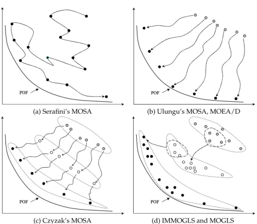
Figure 1: Graphical illustration of different strategies used in multi-objective meta-heuristics based on decomposition.

1990s use weighted aggregation for their acceptance criteria in local search. The main differences between the various MOSA-like algorithms lie in the choice of weights dur-ing the search. The MOSA proposed by Serafini (1992) is a sdur-ingle-point method that optimizes one weighted aggregation function in each iteration (see Figure 1(a)). In this method, the current weight vector is smoothly changed as the search progresses. Similarly, IMMOGLS and MOGLS optimize a single weighted aggregation function in each iteration (see Figure 1(d)). In contrast, two MOSA-like algorithms (Ulungu et al., 1999; Czyzak and Jaszkiewicz, 1998) are population-based search methods and opti-mize multiple weighted aggregation functions (see Figure 1(b) and (c)). In Ulungu’s MOSA, a set of evenly-spread fixed weights is needed, while Czyzak’s MOSA adap-tively tunes the weight vector of each individual according to its location with respect to the nearest non-dominated neighbor.

In Zhang and Li (2007), a multi-objective evolutionary algorithm based on decom-position, called MOEA/D, was proposed. It optimizes multiple subproblems simul-taneously by evolving a population of individuals. In this algorithm, each individual corresponds to one subproblem for which a weighted aggregation function is defined. Like Ulungu’s MOSA, MOEA/D uses fixed weights during the whole search. Since subproblems with similar weight vectors have optimal solutions close to each other, MOEA/D optimizes each subproblem by using the information from the optimiza-tion of neighboring subproblems. For this purpose, recombinaoptimiza-tion and competioptimiza-tion

between neighboring individuals are taken into consideration for mating restriction. Unlike other EMO algorithms, MOEA/D provides a general framework which allows the application of any single objective optimization technique to its subproblems.

In Li and Landa-Silva (2008), we proposed a preliminary approach hybridizing MOEA/D with simulated annealing. In the present work, competition and adapta-tion of search direcadapta-tions are incorporated to develop an effective hybrid evoluadapta-tionary approach, called EMOSA. In the proposed algorithm, the current solution of each sub-problem is improved by simulated annealing with different temperature levels. Af-ter certain low temperature levels, the weight vectors of subproblems are modified in the same way as Czyzak’s MOSA. Contrary to the original MOEA/D, no crossover is performed in our hybrid approach. Instead, diversity is promoted by allowing uphill moves following the simulated annealing rationale.

The hybridization of population-based global search coupled with local search is the main idea of many memetic algorithms (also called genetic local search), which have shown considerable success in single objective combinatorial optimization (Merz, 2000; Krasnogor, 2002; Hart et al., 2004). In these algorithms, genetic search is used to explore promising areas of the search space (diversification) while local search is ap-plied to examine high-quality solutions in a specific local area (intensification). There have also been some extensions of memetic algorithms for multi-objective combinato-rial optimization (Knowles and Corne, 2004).

In some well-known multi-objective memetic algorithms based on decomposi-tion, such as MOGLS and MOEA/D, two basic strategies (random weights and fixed weights) have been commonly used to maintain diversity of search directions towards the POF. However, both strategies have their disadvantages. On the one hand, ran-dom weights might provoke the population to get stuck in local POF or approximate the same parts of the POF repeatedly. On the other hand, fixed weights might not be able to cover the whole POF well. In Czyzak and Jaszkiewicz (1998), the dispersion of non-dominated solutions over the POF is controlled by tuning the weights adaptively.

In our previous work (Li and Landa-Silva, 2008), the weight vector of each indi-vidual is modified on the basis of its location with respect to the closest non-dominated neighbor when the temperature goes below certain level. The value of each component in the weight vector is increased or decreased by a small value. However, the diversity of all weight vectors was not considered. The modified weight vector could be very close to others if the change is too big. In this case, the aggregation function with the modified weights might not be able to guide the search towards unexplored parts of the POF. To overcome this weakness, the adaptation of each weight vector should consider the diversity of all weight vectors in the current population.

As shown in Li and Zhang (2009), competition between solutions of neighboring subproblems in MOEA/D could affect the diversity of the population. Particularly, when the population is close to the POF, the competition between neighboring solu-tions provokes duplicated individuals in the population. Then, in some cases, compe-tition should not be encouraged. For this reason, we need an adaptive mechanism to control competition at different stages during the search.

Like in many multi-objective metaheuristics, MOEA/D uses an external popula-tion to store non-dominated solupopula-tions. When the POF is very large, maintaining such population is computationally expensive. No diversity strategy is adopted to control

the size of the external population in MOEA/D. Popular diversity strategies are crowd-ing distance in NSGA-II and the nearest neighbor method in SPEA-II. Both strategies have computational complexity of at least O(L2_{), where L is the current size of the}

external population. Theǫ-dominance concept is a commonly-used technique for fit-ness assignment and diversity maintenance (Grosan, 2004; Deb et al., 2005). We use

ǫ-dominance within EMOSA to maintain the diversity of the external population of non-dominated solutions.

4

Description of EMOSA

In this section, we propose EMOSA, a hybrid adaptive evolutionary algorithm that combines MOEA/D and simulated annealing. Like in MOEA/D, multiple single objec-tive subproblems are optimized in parallel. For each subproblem, a simulated anneal-ing based local search is applied to improve the current solution. To diversify the search towards different parts of the POF, the weight vectors of subproblems are adaptively modified during the search. The main features of EMOSA include: 1) maintenance of adaptive weight vectors; 2) competition between individuals with respect to both weighted aggregation and Pareto dominance; 3) use ofǫ-dominance for updating the external population. In this section, we first present the main algorithmic framework of EMOSA and then discuss its algorithmic component in more detail.

4.1 Algorithmic Framework

Procedure 1 EMOSA

1: initializeQweight vectorsΛ ={λ(1), . . . , λ(Q)}bySelectWeightVectors(Q) 2: generateQinitial individuals POP={x(1)_{, . . . , x}(Q)_{}randomly or using heuristics}

3: initialize external population EP with non-dominated solutions in POP

4: initialize the temperature setting:T ←Tmax,α←α1

5: repeat

6: for alls∈ {1, . . . , Q}do

7: calculate the neighborhoodΛ(s)for thes-th weight vectorλ(s)

8: end for

9: repeat

10: estimate the nadir pointznad_{and the ideal pointz}∗_{using EP}

11: for alls∈ {1, . . . , Q}do

12: applySimulatedAnnealing(x(s)_{, λ}(s)_{, T)tox}(s)_{and obtainy}

13: competeywith the current population POP byUpdatePopulation(y, s)

14: end for

15: decrease the current temperature value byT ←T×α

16: untilT < Tmin

17: for alls∈ {1, . . . , Q}do

18: modify the weight vectorλ(s)_{byAdaptWeightVectors(s)}

19: end for

20: reset the temperature settings:T ←Treheatandα←α2

21: untilstopping conditions are satisfied

22: return EP

the current set ofQ weight vectorsΛ = {λ(1)_{, . . . , λ}(Q)_{} and the candidate setΘ of}

weight vectors; 2) the current population POP={x(1)_{, . . . , x}(Q)_{}and the external}

pop-ulation EP. The candidate weight vectors inΘare generated by using uniform lattice points (see details in Section 4.2). The size ofΘis much larger thanQ. The total number of weight vectors in the current weight setΛequals the population sizeQsince each individual is associated to one weight vector.

The framework of EMOSA is shown inProcedure 1. Note thatΘ, Λ, POP, and EP are global memory structures, which can be accessed from any subprocedure of EMOSA. In the following, we explain the main steps in EMOSA.

1. The initial weight vectors and population are generated in lines 1 and 2. The ex-ternal population EP is formed with the non-dominated solutions in POP (line 3). 2. For each weight vectorλ(s)_{, the associated neighborhoodΛ(s)is computed based}

on the distance between weight vectors in lines 6-8. Once the current temperature levelT goes below the final temperature levelTmin, the neighborhood should be updated.

3. The nadir and ideal points are estimated using all non-dominated solutions in EP (line 10). More precisely, fmax

i = maxx∈EPfi(x), fimin = minx∈EPfi(x),

i= 1, . . . , m. These two points are used in the setting ofǫ-dominance.

4. For each individual in the population, simulated annealing local search is applied for improvement (line 12). The resulting solutionyis then used to update other individuals in the population (line 13).

5. If the current temperatureTis below the final temperatureTmin, the weight vector of each individual is adaptively modified (lines 17-19).

6. In line 4, the current temperature levelTis set toTmax(starting temperature level), and the current cooling rate is set to be α1 (starting cooling rate). The current

temperature is decreased in a geometric manner (line 15). To help the search escape from the local optimum, the current temperature is re-heated (line 20) toTreheat (< Tmax) and a faster annealing scheme is also applied withα=α2(< α1).

More details of the main steps in EMOSA are given in the following sections.

4.2 Generation of Diverse Weight Vectors

Here,Θis the set of all normalized weight vectors with components chosen from the set: {0,1/H, . . . ,(H −1)/H,1}, withH a positive integer number. The size ofΘ isC_Hm₊−_m1₋₁, withmthe number of objectives. Figure 2 shows a set of 990 uniformly-distributed weight vectors produced using this method forH= 43andm= 3.

In the initialization stage of EMOSA,Qinitial weight vectors evenly spread are selected from the candidate weight setΘ. Note that the size ofΘis much larger thanQ. This procedureSelectWeightVectorsis shown inProcedure 2. In lines 1-3, the extreme weight vectors are generated. Each of these extreme weight vectors corresponds to the optimization of a single objective. In line 4,cis the number of weight vectors selected so far and all selected weight vectors are copied into a temporary setΦ. In line 6, the setAof all weight vectors inΘwith the same maximal distance toΦare identified. In

0 0.5 1 0 0.5 1 0 0.2 0.4 0.6 0.8 1 λ₁ λ₂ λ3

Figure 2: 990 uniform weight vectors.

0 0.5 1 0 0.5 1 0 0.2 0.4 0.6 0.8 1 λ₁ λ2 λ3

Figure 3: 50 selected weight vectors.

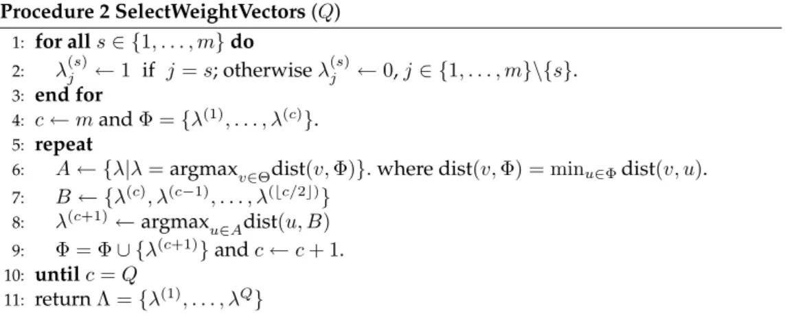
Procedure 2 SelectWeightVectors(Q) 1: for alls∈ {1, . . . , m}do 2: λ(_js)←1 if j=s; otherwiseλ_j(s)←0,j∈ {1, . . . , m}\{s}. 3: end for 4: c←mandΦ ={λ(1)_{, . . . , λ}(c)_}. 5: repeat

6: A← {λ|λ=argmax_v∈Θdist(v,Φ)}.where dist(v,Φ) = minu∈Φdist(v, u).

7: B ← {λ(c)_{, λ}(c−1)_{, . . . , λ}(⌊c/2⌋)_}

8: λ(c+1)←argmax_u∈Adist(u, B)

9: Φ = Φ∪ {λ(c+1)}andc←c+ 1.

10: untilc=Q

11: returnΛ ={λ(1)_{, . . . , λ}Q_}

line 7, the setBis formed with half of the recently selected weight vectors. In line 8, the weight vector inAwith the maximal distance toBis chosen as the next weight vector inΛ. In this way, all weight vectors selected so far are well-distributed. For example, Figure 3 shows the distribution of 50 weight vectors selected from the initial 990 weight vectors shown in Figure 2.

The procedureSelectWeightVectorsinvolvesO(Q2_{× |Θ|)basic operations in lines}

6 and 7 as well asO(|Θ|2_{)distance calculations between the weight vectors inΘ.}

Ide-ally, the large size ofΘleads to a good approximation to the POF since each Pareto optimal solution is the optimal solution of a certain scalarizing function. However, as the size ofΘincreases, the computational complexity ofSelectWeightVectorsand also

AdaptWeightVectors(see details in the next subsection) increase. But, a small size of

Θmight not be enough to approximate the whole Pareto front. To guarantee efficiency,

Hshould be set properly.

In EMOSA, the neighborhood of each weight vector is determined using the same method as in MOEA/D. More precisely, the neighborhoodΛ(s)_ofλ(s)_{fors= 1, . . . , Q,}

is formed by the indexes of itsKclosest neighbors inΛ. Note that the neighborhoods of weight vectors in MOEA/D remain unchanged during the whole search process while those in EMOSA are adaptively changed. This procedure involvesO(Q2_)distance

Figure 4: Weight adaptation in EMOSA.

! "# "$ %&'() % &'*(

Figure 5: Cooling schemes in EMOSA. culations andO(K×Q2_{)basic comparison operators for sorting these distances.}

In Czyzak’s MOSA, the basic idea is to move each non-dominated solution away from its nearest neighbor. To implement this, the weight vectorλof each individual

x is modified at each local move step according to the location of the nearest non-dominated neighbor ofx, lets sayy. The components ofλare changed as follows:

λi=

min{λi+δ,1} if fi(x)< fi(y)

max{λi−δ,0} otherwise (4)

where δ > 0 is the variation level. Note thatλ should be normalized after the above change. However, there are two weaknesses in this method. First, the setting ofδshould be provided empirically. On the one hand, a large value ofδcould push the current solution towards the neighborhood of other solutions. On the other hand, a very small value ofδmight not be able to guide the search towards unexplored ar-eas of the POF. Second, the diversity of all weight vectors in the current population is not considered in setting the value ofλ. This will reduce the chance to approximate different parts of the POF with the same possibility.

Procedure 3 AdaptWeightVectors(s)

1: find the closest non-dominated neighborx(t)_{, t∈ {1, . . . , Q}tox}(s)

2: A← {λ∈Θ|dist(λ(s)_{, λ}(t)_{)<dist(λ, λ}(t)_{)and dist(λ, λ}(s)_{)≤dist(λ,Λ)}}

3: ifA is not emptythen

4: λ(s)←argmax_u∈Adist(u, λ(s))

5: end if

6: returnλ(s)

To overcome the above weaknesses, we introduce a new strategy in EMOSA, il-lustrated in Figure 4, for adapting weight vectors when T < Tmin, i.e. when the

simulated annealing enters the only improving phase. The corresponding

proce-dureAdaptWeightVectorsis shown inProcedure 3. Instead of changing the

compo-nents of the weight vectors, our strategy picks one weight vectorλ from the candi-date set Θto replace the current oneλ(s)_{. For the current solutionx}(s)_{, we need to}

weight vectorλmust satisfy two conditions: 1) dist(λ(s)_{, λ}(t)_{) < dist(λ, λ}(t)_{), and 2)}

dist(λ, λ(s)_{)≤dist(λ,Λ). Condition 1) indicates that the selected weight vector should}

increase the distance between the weight vectors ofx(s)_andx(t)_{. This could cause an}

increase in the distance betweenx(s)andx(t)in the objective space. Condition 2) guar-antees that the selected weight vector should not be too close to other weight vectors in the current population. In line 2 of Procedure 3, all weight vectors inΘsatisfying these two conditions are stored inA. From this set, the weight vector with the maximal distance toλ(s)_{is selected. The procedureAdaptWeightVectorsinvolvesO(Q× |Θ|)}

distance calculations when the current temperature is below the value ofTmin.

4.3 Local Search and Evolutionary Search

In EMOSA, each individual in the population is improved by a local search procedure, namely SimulatedAnnealingshown in Procedure 4. Then, the improved solutions are used to update other individuals in the neighborhood as shown in Procedure 5

UpdatePopulation.

Procedure 4 SimulatedAnnealing(x(s)_{, λ}(s)_{, T)}

1: y←x(s)

2: repeat

3: generate neighboring solutionx′∈ N(y) 4: ifF(x′_{)is not dominated byF(y)then}

5: update EP in terms ofǫ-dominance

6: end if

7: calculate the acceptance probabilityP(y, x′_{, λ}(s)_{, T)}

8: ifP(y, x′_{, λ}(s)_{, T)> random[0,1)then}

9: y←x′

10: end if

11: untilStopping conditions are satisfied

12: returny

In line 3 ofProcedure 4, a neighboring solution x′ _{is generated fromN(y), the}

neighborhood of the current solutiony. IfF(x′_{)is not dominated byF(y), then update}

EP in terms ofǫ-dominance. The components ofǫare calculated byǫi =β×(znadi −

z∗

i), i = 1, . . . , m.Here,β > 0is a parameter to control the density of solutions in EP. The update of EP usingǫ-dominance benefits two aspects: 1) maintain the diversity of EP and 2) truncate the solutions of EP in dense areas of the objective space. In this work,

βis set to 0.002 for two-objective problems and 0.005 for three-objective problems. In the simulated annealing component of EMOSA, the probability of accepting neighboring solutions is given by:

P(x, x′, λ, T) = min{1,exp(−τ×g(x

′_{, λ)−g(x, λ)}

T )} (5)

whereT ∈ (0,1]is the normalized temperature level,τ is a problem-specific balance constant, andgis a weighted aggregation function ofxwith the weight vectorλ, which can be the weighted sum functiong(ws)or the weighted Tchebycheff approachg(te)or the combination of both. According to (5), more uphill (worse) moves are accepted with high probability whenTis close to 1, but increasingly only downhill (better) moves are

accepted asT goes to zero. The acceptance of worse neighboring solutions reduces the possibility of getting trapped in local optima.

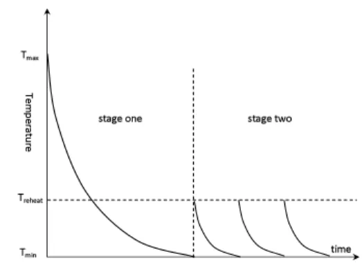
The degree of uphill moves acceptance is determined by the annealing schedule, which is crucial to the performance of simulated annealing. In EMOSA, we apply the following two annealing schedules, shown in Figure 5, in two stages.

• Schedule 1: Before the current temperatureT goes below the final temperature

Tminfor the first time (early stage), local search seeks to improve all individuals using high temperatureTmaxand slow cooling rateα1(line 4 inProcedure 1). This

is the same as many other simulated annealing algorithms. The main task at this stage is to start from the initial population and then quickly find some representa-tive solutions in the POF from the initial population.

• Schedule 2: Whenever the current temperatureTgoes below the final temperature

Tmin(late stage),Tis increased to a medium temperature levelTreheat, and a faster cooling rateα2(< α1)is applied (line 20 inProcedure 1). Since all solutions in the

current population should by now be close to the POF, they should also be close to the optimal solutions of aggregation functions with modified weight vectors. For this reason, there is no need to start a local search from a high temperature level. Fast annealing could help the intensification of the search near the POF since not many uphill moves are allowed.

Moreover, the parameterτin (5) should be set empirically. As suggested in Smith et al. (2004), about half of non-improving neighbors should be accepted at the be-ginning of simulated annealing. Based on this idea, we setτ to−log(0.5)Tmax/∆¯ in EMOSA, where∆¯ is the average of∆gvalues in the first 1000 uphill moves. For these first 1000 uphill moves, the acceptance probability is set to 0.5. In EMOSA, the

Sim-ulatedAnnealing procedure is terminated after examining#lsneighbors. Hence, at

each temperature level, this procedure mainly involvesQ×#lsfunction evaluations and the update of the external population EP.

Note that EMOSA optimizes different subproblems using the same temperature cooling scheme. Actually, each subproblem can also be solved under different cooling schemes. This idea has been used in previous work on simulated annealing algorithm for multi-objective optimization (Tekinalp and Karsli, 2007) and also for single objective optimization (Burke et al., 2001).

Procedure 5 UpdatePopulation(y,s)

1: ifg(y, λ(s)_{)< g(x}(s)_{, λ}(s)_)then

2: x(s)←y

3: end if

4: for allk∈Λ(s)andk6=sdo

5: ifF(y)dominatesF(x(k))then 6: x(k)_←y

7: end if

8: end for

The key difference between EMOSA and other population-based MOSA-like al-gorithms, such as Ulungu and Czyzak’s alal-gorithms, is the competition between indi-viduals. As shown in Li and Zhang (2009), the competition may affect the balance

between diversity and convergence in MOEA/D. On the one hand, the competition among individuals could speed up the convergence towards the POF when the current population is distant to the POF. On the other hand, the competition between individ-uals close to the POF could cause loss of diversity. This is because one solution that is non-dominated with respect to its neighbors could be worse if the comparison is made using a weighted aggregation function. In this paper, we apply different criteria to update the current solution and its neighbors. The details of the process for updat-ing the population are shown inProcedure 5. In lines 1-3, the current solutionx(s)_is

compared to the solutionyobtained by local search and the comparison is made using the weighted aggregation function. In lines 4-8, the neighbors ofx(s)_{are replaced only}

if they are dominated byy. By doing this, the selection pressure among individuals is weak when the current population is close to the POF. Therefore, the diversity of individuals in the neighborhood can be preserved.

5

Two Benchmark MOCO Problems

In this paper, we consider two N P-hard MOCO test problems, the multi-objective knapsack problem and the multi-objective traveling salesman problem. These prob-lems have been widely used when testing the performance of various multi-objective metaheuristics (Jaszkiewicz, 2002; Zhang and Li, 2007; Paquete and St ¨utzle, 2003; Garcia-Martinez et al., 2007; Li et al., 2010).

5.1 The 0-1 Multi-objective Knapsack Problem

Givennitems andmknapsacks, the 0-1 multi-objective knapsack problem (MOKP) can be formulated as:

maximize fi(x) =Pn

j=1pijxj, (6)

subject to Pn

j=1wijxj≤ci, i= 1, . . . , m (7)

wherex = (x1, . . . , xn)is a binary vector. That is,xj = 1if itemj is selected to be included in themknapsacks andxj = 0otherwise,pij andwij are the profit and weight of itemjin knapsacki, respectively, andciis the capacity of knapsacki.

Due to the constraint on the capacity of each knapsack, the solutions generated by local search moves or genetic operators could be infeasible. One way to deal with this is to design a heuristic for repairing infeasible solutions. Some repair heuristics have been proposed in the literature (Zitzler and Thiele, 1999; Zhang and Li, 2007). In this paper, we use the same greedy heuristic adopted in Zhang and Li (2007) for constraint handling. The basic idea is to remove some items with heavy weights and little contribution to an objective function from the overfilled knapsacks.

In Knowles and Corne (2000b), neighboring solutions for the MOKP are produced by flipping each bit in the binary vector with probabilityk/n, calledk-bit flipping here. For example, if thej-th bit ofxis chosen for flipping, thenxj = 1−xj. After flipping, the modified solutionxmight be infeasible and a repair heuristic might be needed. In this paper, we suggest a new neighborhood structure,k-bit insertion, in which only the bits equal to zero may be flipped. This means that more items are added into the knap-sacks but no items are removed. Consequently, the modified solution after flipping bits

with value of zero is very likely to be infeasible but will have higher profits. Then, the repair heuristic is called to remove some items as described above until the solution becomes feasible again.

5.2 The Multi-objective Traveling Salesman Problem

The Traveling Salesman Problem (TSP) can be modeled as a graphG(V, E), whereV =

{1, . . . , n}is the set of vertices (cities) andE={ei,j}n×nis the set of edges (connections between cities). The task is to find a Hamiltonian cycle of minimal length, which visits each vertex exactly once. In the case of the multi-objective TSP (MOTSP), each edgeei,j is associated with multiple values such as cost, length, traveling time, etc. Each of them corresponds to one criterion. Mathematically, the MOTSP can be formulated as:

minimizefi(π) = n−1

X

j=1

c(_πi₍)_j),π(j+1)+c(_πi₍₁₎) _,π(n) i= 1, . . . , m (8)

whereπ = (π(1), . . . , π(n))is a permutation of cities inΠ, the set of all permu-tations of I = {1, . . . , n} and cs,t(i), s, t ∈ I is the cost of the edge between citysand citytregarding criterioni. Unlike the MOKP problem, no repair strategy is needed for solutions to the MOTSP problem because all permutations represent feasible solutions. Like in the single objective TSP problem, the neighborhood move used here for the MOTSP is the 2-opt local search procedure constructed in two steps: 1) remove two non-adjacent edges from the tour and then 2) reconnect vertices associated with the removed edges to produce a different neighbor tour.

6

Computational Experiments

In this section, we experimentally compare the proposed EMOSA to three other MOSA-like algorithms, namely SMOSA (Serafini, 1992), UMOSA (Ulungu et al., 1999), CMOSA (Czyzak and Jaszkiewicz, 1998) and three MOMA-like algorithms, namely MOEA/D (Zhang and Li, 2007), MOGLS (Jaszkiewicz, 2002), and IMMOGLS (Ishibuchi et al., 2003). All algorithms were implemented in C++. We ran all experiments on a PC Pentium CPU (Duo Core) 1.73 GHZ with 2GB memory.

6.1 Performance Indicators

The performance assessment of various algorithms is one of the most important issues in the EMO research. It is well established that the quality (in the objective space) of approximation sets should be evaluated on the basis of two criteria: the closeness to the POF (convergence) and the wide and even coverage of the POF (diversity). In this paper, we use the following two popular indicators for comparing the performance of the multi-objective metaheuristics under consideration.

6.1.1 Inverted Generational Distance (IGD-metric)

This indicator (see Coello Coello and Cruz Cort´es (2005)) measures the average distance from a set of reference pointsP∗ _{to the approximation setP. It can be formulated as}

Table 1: Test instances of MOKP and MOTSP and computational cost.

MOKP MOTSP

Instance n m # nfes Instance n m # nfes

KS2502 250 2 75000 KROAB50 50 2 500000 KS5002 500 2 100000 KROCD50 50 2 500000 KS7502 750 2 125000 KROAB100 100 2 2500000 KS2503 250 3 100000 KROCD100 100 2 2500000 KS5003 500 3 125000 KROABC100 100 3 5000000 KS7503 750 3 150000 KROBCD100 100 3 5000000

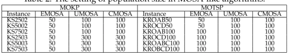
Table 2: The setting of population size in MOSA-like algorithms.

MOKP MOTSP

Instance EMOSA UMOSA CMOSA Instance EMOSA UMOSA CMOSA

KS2502 50 100 100 KROAB50 50 100 100 KS5002 50 100 100 KROCD50 50 100 100 KS7502 50 100 100 KROAB100 100 100 100 KS2503 50 300 300 KROCD100 100 100 100 KS5003 50 300 300 KROABC100 100 100 100 KS7503 50 300 300 KROBCD100 100 100 100 IGD(P, P∗_{) =} 1 |P∗| P

u∈P∗minv∈Pdist(u, v). Ideally, the reference set should be the

whole true POF. Unfortunately, the true POF of many MOCO problems is unknown in advance. Instead, a very good approximation to the true POF can be used. In this paper, the reference setsP∗_{are formed by collecting all non-dominated solutions obtained by}

all algorithms in all runs. The smaller the IGD-metric value, the better the quality of the approximation setP. To have a lower value of the IGD-metric, the obtained solutions should be close toP∗_{and should not miss any part ofP}∗_{. Therefore, the IGD-metric can}

assess the quality of approximation sets with respect to both convergence and diversity.

6.1.2 Hypervolume (S-metric or Lebesgue measure)

This indicator (see Zitzler and Thiele (1999)) measures the volume enclosed by the ap-proximation setP wrt a reference point r = (r1, . . . , rm). In the case of

minimiza-tion, this metric can be written as S(P, r) = VOL S

u∈PE(u, r)

, where E(u, r) =

{v|ui ≤ vi ≤ ri, i = 1, . . . , m} (i.e. E(u, r) is the hyperplane between two m -dimensional points u and r)2_{. Compared to the reference set required in the} IGD-metric, establishing the reference point in the S-metric is relatively easier and more flexible. In our experiments,rcan be set to be a point dominated by the nadir point:

ri = znadi + 0.5(zinad−ziideal), i = 1, . . . , m.The larger the S-metric value, the better the quality of the approximation setP, which means a smaller distance to the true POF and a better distribution of the approximation set. Similar to the IGD-metric, better S-metric values can be achieved when the obtained solutions are close to the POF and achieve a full coverage of the POF. Therefore, the S-metric also estimates the quality of approximation sets both in terms of convergence and diversity.

6.2 EMOSA vs. MOSA-like Algorithms

6.2.1 Experimental Settings

In this first set of experiments, we used the test instances with two and three objectives shown in Table 1. We used the same following parameters in the annealing schedule of the four algorithms:Tmax = 1.0, Tmin = 0.01, Treheat = 0.1, α1 = 0.8, andα2= 0.5.

Moreover, all four algorithms were allocated the same number of function evaluations

Table 3: Mean and standard deviation of IGD-metric values on MOKP instances.

Instance EMOSA UMOSA CMOSA SMOSA

KS2502 16.2(1.86) 34.0 (2.23) 223.5 (19.54) 30.6 (2.17) KS5002 23.1(1.33) 64.9 (2.31) 382.6 (42.57) 80.5 (3.42) KS7502 32.2(2.10) 102.2 (3.75) 657.1 (68.96) 145.2 (6.54) KS2503 54.2(1.10) 71.0 (1.08) 115.2 (5.17) 78.9 (1.45) KS5003 86.4(1.40) 129.5 (1.80) 325.0 (16.37) 184.6 (5.12) KS7503 110.7(2.56) 193.8 (3.76) 547.7 (36.66) 274.0 (4.68)

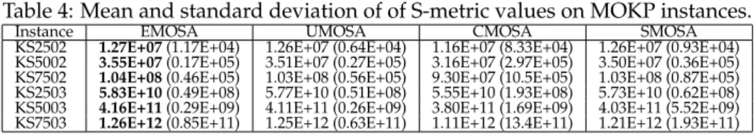
Table 4: Mean and standard deviation of of S-metric values on MOKP instances.

Instance EMOSA UMOSA CMOSA SMOSA

KS2502 1.27E+07(1.17E+04) 1.26E+07 (0.64E+04) 1.16E+07 (8.33E+04) 1.26E+07 (0.93E+04) KS5002 3.55E+07(0.17E+05) 3.51E+07 (0.27E+05) 3.16E+07 (2.97E+05) 3.50E+07 (0.36E+05) KS7502 1.04E+08(0.46E+05) 1.03E+08 (0.56E+05) 9.30E+07 (10.5E+05) 1.03E+08 (0.87E+05) KS2503 5.83E+10(0.49E+08) 5.77E+10 (0.51E+08) 5.55E+10 (1.93E+08) 5.73E+10 (0.62E+08) KS5003 4.16E+11(0.29E+09) 4.11E+11 (0.26E+09) 3.80E+11 (1.69E+09) 4.03E+11 (5.52E+09) KS7503 1.26E+12(0.85E+11) 1.25E+12 (0.63E+11) 1.11E+12 (13.4E+11) 1.21E+12 (1.93E+11)

in each of 20 runs for the same test instance as detailed in column # nfes of Table 1. The population sizes for the three population-based MOSA-like algorithms are given in Table 2. We use a smaller (than in UMOSA and CMOSA) population size in EMOSA for most of the test instances. The reason for this is that EMOSA has the ability to search different parts of the POF by adapting weight vectors. Note that SMOSA is a single point based search method.

At every temperature level, the number #lsof neighbors examined by local search is set to 10 for each MOKP instance and 250 for each MOTSP instance. It should be noted that the total number of neighbors examined in SMOSA at each temperature level equals the total number of neighbors examined for the whole population in UMOSA and CMOSA at the same temperature level. For all test instances in both problems, the neighborhood size in EMOSA is set toK = 10. In both SMOSA and CMOSA, each component of the weight vectors is increased or decreased by2.0/Qrandomly or using the heuristic in eq. (4).

6.2.2 Experimental Results

The mean and standard deviation values of the IGD-metric and S-metric found by the four algorithms are shown in Tables 3 and 4, respectively. From these results, it is evi-dent that EMOSA outperforms the three other MOSA-like algorithms in terms of both performance indicators on all six MOKP test instances. The superiority of EMOSA is due to the stronger selection pressure to move towards the POF by having competition among individuals. We believe that this competition allows the local search in EMOSA to start from a high-quality initial solution at every temperature level.

We can also observe from Tables 3 and 4 that CMOSA is clearly inferior to the three other MOSA-like algorithms. This is due to the fact that CMOSA modifies the weight vector of each individual while examining every neighboring solution. This change of weight vectors in the early stage of the multi-objective search does not affect the distribution of the non-dominated solutions because the current population is still distant to the POF. However, the frequent change of weight vectors could potentially guide each individual to move along different search directions in the objective space. Of course, this will slow down the convergence speed towards the POF. This is why our proposed EMOSA approach only adapts the weight vector of each individual once the temperature is belowTmin.

7500 8000 8500 9000 9500 8000 8500 9000 9500 10000 KS2502 f₁ f2 EMOSA UMOSA CMOSA SMOSA 8900 9000 9100 9200 9300 9200 9300 9400 9500 9600 1.6 1.65 1.7 1.75 1.8 1.85 1.9 1.95 2 x 104 1.65 1.7 1.75 1.8 1.85 1.9 1.95 2 x 104 KS5002 f₁ f2 EMOSA UMOSA CMOSA SMOSA 1.84 1.86 1.88 1.9 x 104 1.9 1.92 1.94 1.96x 10 4 2.4 2.5 2.6 2.7 2.8 2.9 3 x 104 2.3 2.4 2.5 2.6 2.7 2.8 2.9 x 104 KS7502 f₁ f2 EMOSA UMOSA CMOSA SMOSA 2.7 2.75 2.8 x 104 2.75 2.8 2.85 x 104

Figure 6: Non-dominated solutions found by the four MOSA-like algorithms on three bi-objective knapsack instances.

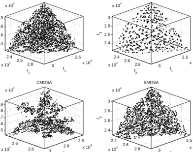
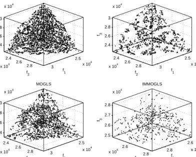
2.5 3 x 10 4 2.4 2.6 2.8 x 104 2.4 2.6 2.8 3 x 104 f 1 EMOSA f₂ f3 2.5 3 x 10 4 2.4 2.6 2.8 x 104 2.4 2.6 2.8 3 x 104 f 1 UMOSA f₂ f3 2.6 2.8 3 x 10 4 2.6 2.8 x 104 2.5 2.6 2.7 2.8 2.9 x 104 f₁ CMOSA f 2 f3 2.5 3 x 10 4 2.4 2.6 2.8 x 104 2.4 2.6 2.8 3 x 104 f₁ SMOSA f 2 f3

Figure 7: Non-dominated solutions found by the four MOSA-like algorithms on the three-objective knapsack instance KS7503.

Table 5: Mean and standard deviation of IGD-metric values on MOTSP instances.

Instance EMOSA UMOSA CMOSA SMOSA

KROAB50 781.20(184.6) 1427.1 (233.7) 12409 (618.3) 6385.5 (447.8) KROCD50 751.54(132.0) 1405.0 (129.9) 11696 (672.0) 6279.6 (392.4) KROAB100 1607.1(234.4) 4327.0 (311.2) 36191 (733.5) 24426 (676.7) KROCD100 1464.8(217.2) 4032.7 (171.3) 35588 (931.8) 23227 (872.3) KROABC100 4421.5(173.3) 5126.9 (143.6) 29819 (659.4) 38646 (473.6) KROBCD100 4253.3(134.8) 4972.0 (150.2) 29008 (626.2) 37269 (460.1)

Table 6: Mean and standard deviation of S-metric values on MOTSP instances.

Instance EMOSA UMOSA CMOSA SMOSA

KROAB50 7.46E+11(5.32E+10) 5.44E+11 (3.83E+10) 2.43E+11 (2.72E+10) 3.00E+11 (3.31E+10) KROCD50 9.83E+11(5.96E+10) 7.88E+11 (3.65E+10) 3.47E+11 (3.0E+10) 4.33E+11 (4.16E+10) KROAB100 4.25E+12(2.66E+11) 3.71E+12 (2.58E+11) 2.10E+12 (1.42E+11) 2.06E+12 (2.42E+11) KROCD100 4.00E+12(2.39E+11) 3.45E+12 (3.09E+11) 1.84E+12 (1.05E+11) 1.77E+12 (1.68E+11) KROABC100 9.12E+20(7.0E+19) 7.32E+20 (4.57E+19) 3.06E+20 (2.86E+19) 1.40E+20 (1.79E+19) KROBCD100 9.12E+20(6.02E+10) 7.35E+20 (4.65E+10) 2.95E+20 (2.81E+19) 1.34E+20 (2.14E+19)

Figure 6 shows the non-dominated solutions found by the four algorithms on three bi-objective MOKP instances for the run for which each algorithm achieved its best value for the IGD-metric. We can see that EMOSA clearly found better solutions than the other three MOSA-like algorithms on KS5002 and KS7502. For the smallest instance KS2502, EMOSA is only slightly better. Moreover, both UMOSA and SMOSA perform quite similarly on these three instances while CMOSA has the tendency to locate the non-dominated solutions close to the middle part of the POF.

In Figure 7, we plot the non-dominated solutions obtained by the four algorithms on the largest MOKP instance with three objectives (KS7503) in the run for which each algorithm achieved its best value for the IGD-metric. It is clear that EMOSA produced the non-dominated front with the best diversity while the non-dominated front by CMOSA has the worst distribution. This is because EMOSA tunes the weight vec-tors according to distances of both objective vecvec-tors and weight vecvec-tors to maintain the diversity of the set of current weight vectors, which are less likely to be very similar. In contrast, CMOSA is unable to preserve the diversity of weight vectors particularly in the case of test instances with more than two objectives.

From Figure 7, we can also note that the set of non-dominated solutions found by UMOSA consists of many isolated clusters. This is because this MOSA-like algorithm with fixed weights has no ability to approximate all parts of the POF when the size of this front is very large. However, it can still produce a good approximation to the POF. This is why EMOSA uses fixed weights only in the early stage of its search pro-cess. It should be pointed out that the population size used in UMOSA and CMOSA is six times that of EMOSA for all 3-objective instances (50 vs. 300). This also demon-strates the efficiency of the strategy for adapting weights in EMOSA which requires a considerably smaller population size.

Tables 5 and 6 show the mean and standard deviation values of the IGD-metric and S-metric obtained by the four MOSA-like algorithms on the six MOTSP instances. Again, EMOSA performs better than the other three MOSA-like algorithms on all six MOTSP test instances in terms of the IGD-metric and the S-metric. In contrast, CMOSA shows again the worst performance.

Figure 8 shows the distributions of the non-dominated solutions obtained by the four MOSA-like algorithms in the run for which each algorithm achieved its best value for the IGD-metric value. It is clear that EMOSA found better non-dominated

solu-Table 7: The average running time (seconds) of four MOSA-like algorithms on two 100-city MOTSP instances.

Instance EMOSA UMOSA CMOSA SMOSA

KROAB100 6.7 3.4 31.2 13.7

KROABC100 169.3 127.4 142.0 39.0

tions in terms of both convergence and diversity. Figure 9 shows the non-dominated solutions obtained in the best run of each algorithm for the threeobjective instance -KROABC100. It can be seen that the diversity of the solutions found by EMOSA is the best among the four algorithms.

From all above results, we can also conclude that the overall performance of UMOSA is better than that of CMOSA and SMOSA for both problems. These results are also consistent with those reported in previous studies (Banos et al., 2007). The poor performance of CMOSA and SMOSA is caused by the frequent modification of weight vectors, which might slow down the convergence speed.

The four MOSA-like algorithms use different strategies to maintain the diversity of weight vectors. The running times of these algorithms rely on the computational complexity of the related strategies. Table 7 shows the average computational time used by the four MOSA-like algorithms on two 100-city MOTSP instances. From this table, we can make the following observations:

• For the smaller 2-objective instance KROAB100, UMOSA is the fastest algorithm while CMOSA is the slowest. This is because UMOSA maintains a set of fixed weight vectors which does not have a computational cost because it is not required to tune the weight vectors. In contrast, both CMOSA and SMOSA modify weight vectors at each single local search move. The computational complexity of the strategy in CMOSA is much higher than that in SMOSA, however EMOSA is still faster. Therefore, it seems that it is not reasonable to tune the weight vectors at every local search move.

• For the larger 3-objective instance KROABC100, both EMOSA and UMOSA are slower than SMOSA. This is contrary to the above observation. The reason for this is that the the number of non-dominated solutions found by the former two algorithms is much larger than those found by SMOSA. In this case, most of the computational cost is allocated to maintaining the external population. This is also the reason why CMOSA is faster than EMOSA.

6.3 EMOSA vs. MOMA-like Algorithms

6.3.1 Experimental Settings

In this section, we compare EMOSA to three MOMA-like algorithms, namely MOEA/D, MOGLS, and IMMOGLS. All parameter settings used in EMOSA are the same as in the previous section. The population sizes used in the other three algo-rithms are given in Table 8. Like EMOSA, the neighborhood size used in MOEA/D is also 10 for all test instances. In MOGLS, the size of the mating pool is set to 20 for every test instance. In IMMOGLS, 10 elite solutions are randomly selected from the external

2 3 4 5 6 7 8 x 104 2 3 4 5 6 7 x 104 KROAB50 f₁ f2 EMOSA UMOSA CMOSA SMOSA 3 3.5 4 x 104 2.5 3 3.5 x 104 4 6 8 10 12 14 16 x 104 4 6 8 10 12 14 16 x 104 KROAB100 f₁ f2 EMOSA UMOSA CMOSA SMOSA 5 6 7 x 104 5 6 7 x 104 2 3 4 5 6 7 x 104 2 3 4 5 6 7 8 x 104 KROCD50 f₁ f2 EMOSA UMOSA CMOSA SMOSA 2.6 2.8 3 3.2 3.4 3.6 3.8 x 104 3 3.5 4 x 104 4 6 8 10 12 14 16 x 104 4 6 8 10 12 14 x 104 KROCD100 f₁ f2 EMOSA UMOSA CMOSA SMOSA 5 6 7 x 104 4.5 5 5.5 6 6.5 x 104

Figure 8: The non-dominated solutions found by MOSA-like algorithms on bi-objective MOTSP instances. 5 10 15 x 10 4 5 10 15 x 104 5 10 15 x 104 f 1 EMOSA f₂ f3 0.5 1 1.5 x 10 5 0.5 1 1.5 x 105 0.5 1 1.5 x 105 f 1 UMOSA f₂ f3 0.5 1 1.5 x 105 0.5 1 1.5 x 105 0.5 1 1.5 x 105 f₁ CMOSA f 2 f3 0.6 0.8 1 1.2 1.4 x 10 5 0.6 0.8 1 1.2 1.4 x 105 0.6 0.8 1 1.2 1.4 x 105 f₁ SMOSA f 2 f3

Figure 9: The non-dominated solutions found by MOSA-like algorithms on instance KROABC100.

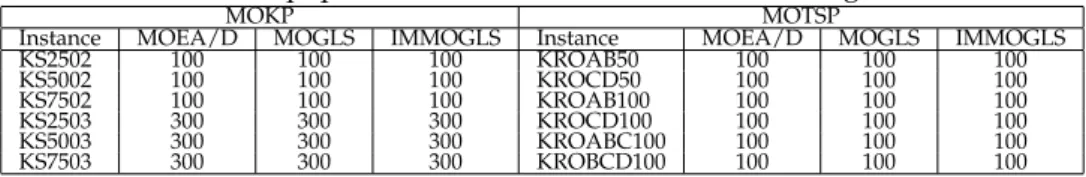
Table 8: The population size used in the MOMA-like algorithms.

MOKP MOTSP

Instance MOEA/D MOGLS IMMOGLS Instance MOEA/D MOGLS IMMOGLS

KS2502 100 100 100 KROAB50 100 100 100 KS5002 100 100 100 KROCD50 100 100 100 KS7502 100 100 100 KROAB100 100 100 100 KS2503 300 300 300 KROCD100 100 100 100 KS5003 300 300 300 KROABC100 100 100 100 KS7503 300 300 300 KROBCD100 100 100 100

Table 9: Mean and standard deviation of IGD-metric values found by MOMA-like al-gorithms on MOKP instances.

Instance EMOSA MOEA/D MOGLS IMMOGLS

KS2502 16.2(1.86) 24.0 (4.42) 21.5 (4.70) 100.5 (15.23) KS5002 23.1(1.33) 64.3 (5.82) 55.6 (2.88) 292.8 (29.68) KS7502 32.2(2.10) 157.5(10.87) 134.6(9.08) 620.3 (40.70) KS2503 54.2(1.10) 66.6 (1.68) 56.4 (2.0) 252.1 (23.12) KS5003 86.4(1.40) 166.6(4.11) 134.8(3.84) 734.1 (59.79) KS7503 110.7(2.56) 334.5(12.77) 233.3(5.20) 1160.7(44.70)

population. For the MOKP problem, single-point crossover is performed, and each bit of the binary string is mutated by flipping with probability 0.01. The neighborhood structures for both the MOKP problem and the MOTSP problem are the same as in the previous section. For the MOTSP instances, offspring solutions are sampled by using cycle crossover (Larranaga et al., 1999) in these three MOMA-like algorithms.

6.3.2 Experimental Results

The mean and standard deviation of the IGD-metric and S-metric values found by EMOSA and the three MOMA-like algorithms on six MOKP test instances are shown in Table 9 and Table 10, respectively. From this set of results, it is evident that EMOSA performs better than the three MOMA-like algorithms on all test instances. We think that the superiority of EMOSA is due to i) the use of a diverse set of weight vectors and ii) the use of simulated annealing for local search.

Among the four algorithms, IMMOGLS has the worst performance on all test in-stances. This is because IMMOGLS uses a fixed population size and updates the current population with all offspring solutions without competition. In EMOSA, individuals with similar weight vectors interact with each other via competition, which helps for a good performance of EMOSA in terms of convergence.

Zhang and Li (2007) showed that MOEA/D constantly performs better than MOGLS on the MOKP test instances when local search heuristic is applied. When simple hill-climber local search is used in both algorithms, MOEA/D performs slightly worse than MOGLS regarding the IGD-metric since the population size is not large

Table 10: Mean and standard deviation of S-metric values found by MOMA-like algo-rithms on MOKP instances.

Instance EMOSA MOEA/D MOGLS IMMOGLS

KS2502 1.27E+07(1.17E+04) 1.27E+07(1.34E+04) 1.27E+07(1.12E+04) 1.21E+07(7.73E+04) KS5002 3.55E+07(0.18E+05) 3.51E+07(0.58E+05) 3.51E+07(0.44E+05) 3.21E+07(3.02E+05) KS7502 1.04E+08(0.46E+05) 1.02E+08(1.42E+05) 1.02E+08(1.56E+05) 9.14E+07(10.6E+05) KS2503 5.83E+10(0.49E+08) 5.80E+10(0.59E+08) 5.77E+10(1.10E+08) 4.90E+10(9.31E+08) KS5003 4.16E+11(0.29E+09) 4.07E+11(0.55E+09) 4.04E+11(1.09E+09) 3.10E+11(5.51E+09) KS7503 1.26E+12(0.85E+09) 1.20E+12(2.37E+09) 1.20E+12(3.57E+09) 8.87E+11(15.1E+09)

7500 8000 8500 9000 9500 7500 8000 8500 9000 9500 10000 KS2502 f₁ f2 EMOSA MOEA/D MOGLS IMMOGLS 8900 9000 9100 9200 9300 9200 9300 9400 9500 9600 1.6 1.65 1.7 1.75 1.8 1.85 1.9 1.95 2 x 104 1.65 1.7 1.75 1.8 1.85 1.9 1.95 2 x 104 KS5002 f₁ f2 EMOSA MOEA/D MOGLS IMMOGLS 1.84 1.86 1.88 1.9 x 104 1.9 1.92 1.94 1.96 x 104 2.4 2.5 2.6 2.7 2.8 2.9 3 x 104 2.3 2.4 2.5 2.6 2.7 2.8 2.9 x 104 KS7502 f₁ f2 EMOSA MOEA/D MOGLS IMMOGLS 2.7 2.75 2.8 x 104 2.72 2.74 2.76 2.78 2.8 2.82 2.84x 10 4

Figure 10: Non-dominated solutions found by MOMA-like algorithms on bi-objective knapsack instances. 2.5 3 x 10 4 2.4 2.6 2.8 x 104 2.4 2.6 2.8 3 x 104 f 1 EMOSA f₂ f3 2.5 3 x 10 4 2.4 2.6 2.8 x 104 2.4 2.6 2.8 3 x 104 f 1 MOEA/D f₂ f3 2.5 3 x 10 4 2.4 2.6 2.8 x 104 2.4 2.6 2.8 3 x 104 f₁ MOGLS f 2 f3 2.6 2.8 x 104 2.6 2.8 x 104 2.5 2.6 2.7 2.8 x 104 f₁ IMMOGLS f 2 f3

Figure 11: Non-dominated solutions found by MOMA-like algorithms on the KS7503 instance.

Table 11: Mean and standard deviation of IGD-metric values found by MOMA-like algorithms on MOTSP instances.

Instance EMOSA MOEA/D MOGLS IMMOGLS

KROAB50 781.2(184.6) 1253.8(219.7) 3574.7(620.7) 8412.4(923.9) KROCD50 751.5(132.0) 1220.9(201.2) 3744.7(430.4) 8182.6(851.6) KROAB100 1607.1(234.4) 2184.5(258.7) 17100(1524) 24052(1156) KROCD100 1464.8(217.2) 2030.9(307.2) 16337(930) 22840(2050) KROABC100 4421.5(173.3) 6126.6(254.8) 22789(868) 34419(831.6) KROBCD100 4253.3(134.8) 6189.3(236.4) 22079(963) 33475(1291.4)

Table 12: Mean and standard deviation of S-metric values found by four MOMA algo-rithms on six MOTSP instances.

Instance EMOSA MOEA/D MOGLS IMMOGLS

KROAB50 7.46E+11(5.33E+10) 5.98E+11(5.44E+10) 3.62E+11(7.07E+10) 1.97E+11(2.72E+10) KROCD50 9.83E+11(5.96E+10) 8.31E+11(5.68E+10) 5.02E+11(6.69E+10) 3.02E+11(5.12E+10) KROAB100 4.25E+12(2.66E+11) 3.37E+12(3.11E+10) 1.84E+12(1.62E+11) 1.59E+12(2.25E+11) KROCD100 4.01E+12(2.39E+11) 3.20E+12(2.90E+11) 1.49E+12(2.36E+11) 1.35E+12(2.06E+11) KROABC100 9.12E+20(7.00E+19) 2.63E+20(1.80E+19) 1.32E+20(2.75E+19) 8.82E+19(2.17E+19) KROBCD100 9.12E+20(6.03E+19) 2.45E+20(1.99E+19) 1.13E+20(2.70E+19) 7.91E+19(2.03E+19)

enough, but better in terms of the S-metric. In contrast, EMOSA clearly outperforms MOGLS, which gives an indication that the use of advanced local search based meta-heuristics can enhance the performance of EMO algorithms.

The final solutions found by EMOSA and the three MOMA-like algorithms on three 2-objective MOKP instances are plotted in Figure 10. For KS2502, EMOSA per-forms similarly to MOEA/D and MOGLS. However, the solutions found by EMOSA are better than those obtained by MOEA/D and MOGLS on two larger test instances KS5002 and KS7502. It is clear that the solutions of IMMOGLS are dominated by those of the other three algorithms.

Figure 11 shows the solutions found by the four algorithms on instance KS7503 for the run in which each algorithm achieved the best IGD-metric value. It is evident that EMOSA has the best performance wrt diversity. In MOEA/D, the non-dominated solutions are located in a number of clusters. This is because MOEA/D uses fixed weights during the whole search process. Therefore, the performance of MOEA/D depends on the population size. For large test instances, a reasonable large number of weight vectors is required to achieve good diversity in the final non-dominated set of solutions. However, although the population size in EMOSA is small, this algorithm is still capable of solving large test instances due to the effective adaptation of weight vectors.

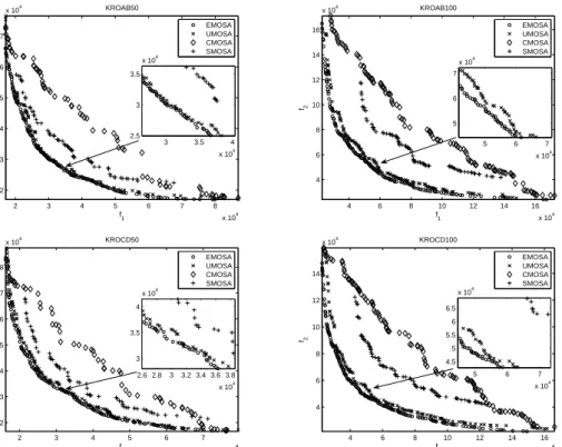
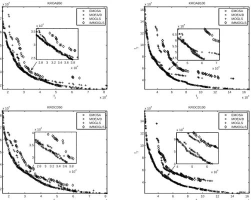
Table 11 and Table 12 give the mean and standard deviation of IGD-metric and S-metric values found by EMOSA and the three MOMA-like algorithms on six MOTSP test instances. From these experimental results, it is clear that EMOSA found the best solutions in terms of both indicators. Figure 12 shows the distribution of the solutions obtained by the four algorithms on four bi-objective MOTSP test instances. As we can see, both EMOSA and MOEA/D have good performance in terms of convergence. The solutions found by both algorithms are quite close to each other. As for diversity, the distribution of the solutions found by EMOSA is more uniform. Both MOGLS and IMMOGLS have worse performance than EMOSA in all test instances. This could be due to the lack of efficient genetic operators for sampling promising offspring solutions for multi-objective local search.

2 3 4 5 6 7 8 x 104 2 3 4 5 6 7 x 104 KROAB50 f₁ f2 EMOSA MOEA/D MOGLS IMMOGLS 2.8 3 3.2 3.4 3.6 3.8 x 104 2.5 3 3.5 x 104 4 6 8 10 12 14 16 x 104 4 6 8 10 12 14 16 x 104 KROAB100 f₁ f2 EMOSA MOEA/D MOGLS IMMOGLS 5 6 7 x 104 4.5 5 5.5 6 6.5 x 104 2 3 4 5 6 7 8 x 104 2 3 4 5 6 7 8 x 104 KROCD50 f₁ f2 EMOSA MOEA/D MOGLS IMMOGLS 2.8 3 3.2 3.4 3.6 3.8 x 104 3 3.5 4 x 104 4 6 8 10 12 14 16 x 104 4 6 8 10 12 14 x 104 KROCD100 f₁ f2 EMOSA MOEA/D MOGLS IMMOGLS 4 5 6 x 104 4 5 6 x 104

Figure 12: Non-dominated solutions found by MOMA-like algorithms on bi-objective TSP instances.

Figure 13 shows the distribution of the non-dominated solutions found by the four algorithms on the 3-objective KROABC100 instance. Unlike the concave POF of instance KS7503, the POF of instance KROABC100 is convex. We can observe that EMOSA has the best performance in finding a good distribution of non-dominated so-lutions.

7

Effect of Algorithmic Components and Analysis of Parameter Sensitivity

in EMOSA

7.1 Effect of Algorithmic Components

7.1.1 Adaptation of Weight Vectors

In our early work on EMOSA (Li and Landa-Silva, 2008), we tried the same strategy as in CMOSA to adapt weight vectors. As we discussed in section 3, that strategy has some weaknesses. In this section, we demonstrate the improvement of EMOSA due to the new diversity strategy. We modified the EMOSA approach shown inProcedure1 by replacing our weights adaptation strategy with the strategy used in CMOSA and ap-plied the modified algorithm to instance KROABC100. All parameters in this modified EMOSA remain the same as those in section 6.2.1. Figure 14 shows the non-dominated solutions found by this modified EMOSA. Compared to the results in Figure 13, the modified EMOSA performs worse in terms of diversity. This indicates that our new

di-5 10 15 x 10 4 5 10 15 x 104 5 10 15 x 104 f 1 EMOSA f₂ f3 5 10 15 x 10 4 5 10 15 x 104 5 10 15 x 104 f 1 MOEA/D f₂ f3 0.6 0.8 1 1.2 1.4 x 10 5 0.6 0.8 1 1.2 1.4 x 105 0.5 1 1.5 x 105 f₁ MOGLS f 2 f3 0.6 0.8 1 1.2 1.4 x 10 5 0.6 0.8 1 1.2 1.4 x 105 0.8 1 1.2 1.4 x 105 f₁ IMMOGLS f 2 f3

Figure 13: Non-dominated solutions found by MOMA-like algorithms on the KROABC100 instance.

versity strategy works better in guiding the multi-objective search towards unexplored parts of the POF by maintaining the diversity of weight vectors.

7.1.2 Competition Strategies

As we said before, EMOSA distinguishes itself from other algorithms by the adaptive competition scheme between individuals. We carried out three further experiments to study the effect of the competition among individuals on the performance of EMOSA.

To study the effect of weighted aggregation function on the convergence of EMOSA, we compared two versions of EMOSA, one using the weighted sum approach and the other one using the weighted Tchebycheff approach. Both versions use the

0.5 1 1.5 x 10 5 5 10 15 x 104 0.5 1 1.5 x 105 f 1 KROABC100 f2 f3

Figure 14: CMOSA’s diversity strategy.

4 6 8 10 12 14 16 x 104 4 6 8 10 12 14 16 x 104 f 1 f2 KROAB100 5 6 7 x 104 4 5 6 x 104

Weighted Sum approach Weighted Tchebycheff approach

4 6 8 10 12 14 16 x 104 4 6 8 10 12 14 16 x 104 f 1 f2 KROAB100 4.5 5 5.5 6 6.5 x 104 4.5 5 5.5 6 6.5 x 104 Competition No Competition

Figure 16: Effect of competition.

0.5 1 1.5 x 10 5 5 10 15 x 104 0.5 1 1.5 x 105 f 1 KROABC100 f 2 f3

Figure 17: No Pareto selection.

same parameter settings described in Section 6.2.1. Figure 15 shows the non-dominated solutions found by these two versions. From these results, we can observe that the weighted Tchebycheff approach performs very similar to the weighted sum approach on KROAB100. Zhang and Li (2007) made a different observation, that the former has worse performance on the MOKP problem. The reason for this is that the weighted sum approach has higher effectiveness in preserving the quality of infeasible solutions in the repair heuristic.

Also, we tried the version of EMOSA with no competition between individuals. That is, the current solution of each weighted aggregation function does not compete with its neighboring solutions. To implement this, lines 4-8 inProcedure 5were re-moved. We tested this version of EMOSA on the KROAB100 instance using the same parameters as in section 6.2.1. Figure 16 shows the non-dominated solutions found by EMOSA without competition between individuals. Clearly, the convergence of this version is worse than the EMOSA with competition.

Moreover, we tested another version of EMOSA with competition based on only scalarization. InProcedure 5, lines 5-7 were removed. Instead, each neighboring so-lutionx(k)_{is replaced withy ifg(y, λ}(k)_{) < g(x}(k)_{, λ}(k)_{). This variant of EMOSA was}

tested on instance KROABC100. The final solutions found by this variant are plotted in Figure 17. It can be observed that the modified EMOSA failed to find a set of well-distributed non-dominated solutions despite having the adaptation of weight vectors. As mentioned before, this is caused by the loss of diversity in the population. When the current population is close to the POF, neighboring solutions are very likely to be mutually non-dominated. However, one solution can still be replaced by its neighbors in terms of a weighted sum function. In this case, EMOSA might miss the chance to approximate the part of POF nearby such a solution. This is why EMOSA does not work well on KROABC100 wrt diversity.

7.1.3 Choice of Neighborhood Structure

The choice of appropriate neighborhood structure plays a very important role in local search methods for combinatorial optimization. In this paper, we have proposed ak-bit insertion neighborhood structure for the MOKP problem. In this section, we compare two versions of EMOSA on the instance KS2502, one using thek-bit insertion neighbor-hood and another version using thek-bit flipping neighborhood. Figure 18 shows the

7500 8000 8500 9000 9500 8000 8500 9000 9500 10000 f₁ f2 KS2502 k−bit insertion k−bit flipping

Figure 18: k-bit insertion vs. k-bit flipping.

0.5 1 1.5 x 10 5 5 10 15 x 104 0.5 1 1.5 x 105 f 1 KROABC100 f₂ f3

Figure 19: External population update.

final solutions found by both versions in the best of 20 runs regarding the IGD-metric. It can be observed that the non-dominated solutions obtained by EMOSA with thek-bit insertion neighborhood dominate all solutions produced by the version with thek-bit flipping neighborhood. Moreover, the mean IGD-metric value obtained when using thek-bit flipping neighborhood is 76.934, which is worse than the value obtained when using thek-bit insertion (16.245).

7.1.4 Updating the External Population withǫ-dominance

In MOEA/D, no diversity strategy is applied to manage the external population. This is not a problem when the size of the POF is small. However, for large fronts, the ex-ternal population might contain more and more non-dominated solutions as the search progresses. The computational time needed to update the external population may ex-ceed substantially the time used by all other components of EMOSA. This is why we incorporateǫ-dominance into EMOSA to help in keeping the diversity of EP automat-ically. Figure 19 shows the results obtained by EMOSA without usingǫ-dominance on instance KROABC100. Compared to the results in Figure 9, the distribution of non-dominated solutions is more dense that the distribution obtained with EMOSA using

ǫ-dominance. Up to 20,000 non-dominated solutions are saved in the external popu-lation while EMOSA withǫ-dominance reports only about 3000 solutions at the end of each run. In terms of the computational time, we also noticed that EMOSA with-outǫ-dominance used about 1600 seconds to complete one run, while EMOSA with

ǫ-dominance only spent less than 170 seconds to complete a single run, which repre-sents almost a ten-fold reduction.

7.2 Analysis of Parameter Sensitivity

7.2.1 Parameters in Two-stage Cooling Scheme

Like the simulated annealing algorithms for single objective optimization, the per-formance of EMOSA might also be influenced by the setting of parameters in the cooling scheme. To verify this, we studied two parametersTreheat (reheat tempera-ture value) and α2 (fast cooling rate). EMOSA with the combinations of Treheat =

{0.1,0.3,0.5,0.8,1.0}andα2={0.3,0.5,0.8}were tested on KROAB50 and KROAB100