Robustness-Driven Resilience Evaluation of Self-Adaptive Software Systems

Robustness-Driven Resilience Evaluation of

Self-Adaptive Software Systems

Javier C ´amara, Rog ´erio de Lemos, Nuno Laranjeiro, Rafael Ventura, and Marco Vieira

Abstract—An increasingly important requirement for certain classes of software-intensive systems is the ability to self-adapt their structure and behavior at run-time when reacting to changes that may occur to the system, its environment, or its goals. A major challenge related to self-adaptive software systems is the ability to provide assurances of their resilience when facing changes. Since in these systems, the components that act as controllers of a target system incorporate highly complex software, there is the need to analyze the impact that controller failures might have on the services delivered by the system. In this paper, we present a novel approach for evaluating the resilience of self-adaptive software systems by applying robustness testing techniques to the controller to uncover failures that can affect system resilience. The approach for evaluating resilience, which is based on probabilistic model checking, quantifies the probability of satisfaction of system properties when the target system is subject to controller failures. The feasibility of the proposed approach is evaluated in the context of an industrial middleware system used to monitor and manage highly populated networks of devices, which was implemented using the Rainbow framework for architecture-based self-adaptation.

Index Terms—resilience evaluation, self-adaptive systems, robustness testing techniques, probabilistic model checking.

F

1

I

W

any other system is its ability to continuously deliver its services despite changes that may occur in the system, its environment or its goals. A key component that enables

self-adaptive systems to handle changes at run-time is acontroller

that relies on a feedback loop for managing adaptations [1].

Controllers execute actions via effectors on the target system

(i.e., the subsystem managed by the controller), based on information monitored by probes. In the context of complex software systems, these controllers usually consist of four distinct operational stages, namely, Monitor, Analyze, Plan and Execute (MAPE-K [2]) which implement the traditional

sense-plan-act architectures.

Although major advances have been made in this area, existing approaches do not systematically address the need

to determine if a self-adaptive system isresilient(i.e., if it can

deliver a service that can justifiably be trusted when facing

changes[3]), resulting in a lack of widespread adoption.

There is a variety of changes that can have a negative impact on the resilience of a self-adaptive system, including changes in its execution environment (e.g., resource availability) and in the system itself (e.g., faults). Previous work has explored the influence on resilience of a limited subset of system changes, such as failure in the execution of adaptive actions via effectors, or in components of the target system [8]. However, a key subset of undesirable behaviors that remain to be studied in the context of resilience are those that manifest in the • J. C´amara is with the Institute for Software Research, Carnegie Mellon

University, USA. E-mail: [email protected]

• N. Laranjeiro, R. Ventura, and M. Vieira are with the Department of Informatics Engineering, University of Coimbra, Portugal.

E-mail:{ventura, cnl, mvieira}@dei.uc.pt

• R. de Lemos is with the School of Computing, University of Kent, UK, and CISUC, University of Coimbra, Portugal. E-mail: [email protected]

controller (e.g., flaws in adaptation logic, or failures caused by invalid probe inputs). Controllers are prone to misbehave due to their complexity, and can potentially have a significant impact on the resilience of the overall system due to the importance of their function.

This paper proposes a novel approach for systematically evaluating the resilience of self-adaptive systems that embody the MAPE-K model by focusing on the impact that controller failures, caused by malformed inputs from probes, have upon the target system. The approach comprises two phases: 1) Identifying controller failures by injecting invalid inputs at

the controller’s interface (i.e., probes) during the different operational stages of the MAPE-K loop. This phase of the approach is based on a novel technique for robustness testing of MAPE-K-based controllers [5].

2) Quantifying the impact that the identified controller failures have upon the resilience of the target system. Information about the behavior of the target system during different executions is collected in the form of execution traces. These traces replicate controller failure conditions (i.e., environment conditions and input mutations) identified in (1), and are aggregated into a model based on Discrete-Time Markov Chains (DTMCs). We quantify resilience by model checking resilience properties formalized as PCTL formulae [6] on the synthesized DTMC-based models. Resilience measures obtained provide valuable insight that can allow developers to improve system resilience. This can be achieved by explicitly considering in the adaptation logic known situations that lead to controller failure.

Previous work about resilience evaluation of self-adaptive systems [7], [8] dealt with different sources of change that can impact resilience, such as the environment, or the target system itself. Moreover, the frameworks for resilience evalua-tion on which these approaches relied were limited to

non-conventional operational profiles or NCOPs (i.e., situations in which the system experiences an anomaly and requires adaptation). In contrast, the novelty of the approach presented in this paper is dealing with malformed input at the interface between controller and target system (e.g., probes), as a major source of change that can impact resilience. Moreover, the resilience evaluation framework that supports the approach has been extended by:

• Covering the conventional operational profile (COP) case

in which the system operates without the need to adapt. In this situation, controller failures can cause unintended adaptations that might deviate the system from the COP, having a negative impact on resilience. This demands a formalization of resilience properties that differs from the NCOP case (Section 4.2), and a different experimental procedure (Section 4.2.2).

• Refining the NCOP case into two different subcases for

the planning and execution stages of MAPE-K, which requires different procedures when evaluating resilience in the context of controller failures (Section 4.2.2).

The feasibility of the proposed approach is evaluated in the context of an industrial middleware system developed at

Critical Software1_{for monitoring renewable energy production}

plants. We have chosen to use a controller developed using Rainbow for performing the evaluation because its structure facilitates access to the internal components, and the logs Rainbow produces are suitable for analyzing the effects of the robustness tests upon the controller [9]. Our results confirm that the stateful nature of the controller heavily influences the resilience of the system, justifying the need to consider it as a first-order element in robustness testing and resilience evaluation.

The rest of this paper is structured as follows. Section 2 provides some background on self-adaptive systems and re-lated work. Section 3 introduces the case study used for illustrating our approach. Section 4 describes our approach for evaluating the resilience of self-adaptive systems based on robustness testing of the controller. Section 5 presents results. Section 6 discusses limitations of the approach. Finally, Section 7 concludes the paper and indicates future work.

2

B

R

W

Over the past few years, run-time management of increasingly complex software-intensive systems has become a central concern in Software Engineering [11], [12]. A major issue in this area is related to achieving conformance to functional and non-functional requirements in a dependable and cost-effective manner, while changes may affect the system, its environment, and system goals.

One of the proposals addressing this concern was IBM’s Autonomic Computing initiative [2], which has introduced a layer implementing what is known as the MAPE-K control loop to Monitor, Analyze, Plan, and Execute adaptation (with a Knowledge Base acting as a cornerstone of the process) for managing a target system. Some successful approaches that

1. http://www.criticalsoftware.com/

rely on this closed-loop control paradigm exploit architectural models for reasoning about the target system under manage-ment [9], [13]. In particular, Rainbow [9] provides a reusable framework that can be applied to a wide range of systems via customization. Section 5.1 overviews Rainbow, which has been used to build the controller used to validate our approach. Contributions supporting the provision of assurances in self-adaptive systems rely on the analysis of non-functional prop-erties, and are based either on modeling or direct measurement of an existing system. Concerning direct measurement, Epifani

et al.[14] present a framework to keep models alive by feeding

them with run-time data that updates their internal parameters. The framework uses DTMCs and Queuing Networks to reason

about reliability and performance. Calinescuet al.[15], extend

and combine [14] and [16] for defining a framework for the development of adaptive service-based systems. QoS require-ments expressed as probabilistic temporal logic formulas are used to enforce optimal system configurations. Our approach focuses on quantitative analysis using measurements, and does not assume the existence of DTMCs describing system com-ponents. Moreover, while most proposals deal with estimates of the future system behavior for optimizing its operation, our approach focuses on evaluating levels of confidence with respect to the self-adaptive capabilities of the system.

A less restricted notion of operational profile, compared to the one presented in this paper is introduced by Schmeck et

al. in [17], where the notion ofacceptance spaceis analogous

to the COP, consisting in the set of states in which the system is operating without experiencing any disturbances.

Preliminary work considers only environment stimulation as source of change [7], leaving out changes that are internal to the system, which are dealt with in the present paper by exploiting failures that may affect the controller. In a more recent work, an architecture-based approach evaluates by comparison the adaptation mechanisms of a self-adaptive software system [8]. Although these approaches quantitatively measure resilience of the self-adaptive system when facing internal and external changes to the system, they only cover NCOPs (induced by changes in the environment or the target system, e.g., injected faults). The approach presented in this paper extends the aforementioned approaches by incorporating an experimental profile for the system’s COP. Moreover, the NCOP case is refined into two experimental profiles according to the stages in which the controller can be while in a NCOP (i.e., planning, execution).

Another area related to resilience evaluation is resilience benchmarking, which encompasses techniques from previ-ous efforts in performance benchmarking [18], dependabil-ity benchmarking [19], and securdependabil-ity benchmarking [20]. A resilience benchmark is specified following the same basic approach of other types of benchmark, but comprising a changeload (which includes, but is not limited to, faults), as well as resilience metrics [8] [21]. Some of the works on assessment and evaluation of resilience in computer systems presented in [22] are of particular interest:

The authors of [23] describe the state-of-the-art on assessing and comparing the performance, dependability, and security

attributes of systems following standardizing procedures (i.e., benchmarks). This paper contributes a theoretic definition of the components needed to build a resilience benchmark, e.g., metrics, workloads, and perturbation-loads. Perturbation-loads are particularly relevant and, in the context of our work, can be seen as the robustness tests performed.

The work in [24] considers performance degradation as a potential symptom of system instability, which in turn is seen as a resilience issue. The idea consists of: (i) defining a resilience metric that can be derived from security, reliability or performance aspects; (ii) model the system states and associated events using Markov chains; and (iii) use the outputs of the tests to calculate the resilience metric based on the model. The work presented is in a very early stage and focuses only on the characterization of performance as a resilience indicator.

The work in [25] characterises robustness as a resilience attribute and surveys techniques and tools for robustness test-ing in different domains. The chapter proposes the adaptation of the modeling approach presented in [24] to the context of robustness testing. However, the work presented is mostly a review of the state-of-the-art and the proposed approach for resilience modeling and analysis is merely theoretical.

Robustness testing allows the characterisation of the be-haviour of a system or component in the presence of ex-ceptional input conditions. This technique aims at providing feedback about the stimuli that may trigger internal errors in the system under test, helping developers to fix problems that might otherwise go unnoticed.

Ballista [27] uses a set of tests that combine acceptable and exceptional values on calls to kernel functions of operating systems. The parameter values used in each invocation are randomly extracted from a set of predefined tests, and for each parameter, a set of values of a certain data type is associated. Each operating system is classified in terms of its robustness according to a predefined scale that distinguishes several failure modes (the CRASH scale [27]).

MAFALDA (Microkernel Assessment by Fault injection AnaLysis and Design Aid) [28] is a tool that enables the characterisation of the behaviour of microkernels in the pres-ence of faults. Fault injection is performed at two levels: in the parameters of system calls and in the memory segments holding the target microkernel. However, only the former is relevant when the goal is robustness testing.

In previous work, we defined an approach to assess the be-havior of web services accessed via tampered SOAP messages [29]. The approach consists of a set of robustness tests based on invalid web services call parameters. Web services are classified according to failures observed during the execution of the tests using an adaptation of the CRASH scale [27].

The abovementioned works implement robustness testing approaches that do not consider the state of the system under test. In [30] the impact of state on robustness testing of a safety-critical operating system (OS) is investigated by in-cluding the OS state in test cases definition. Although system-specific, results show that the state can play an important role, being able to cover more cases than traditional approaches.

An approach for robustness testing of stateful Web services is presented in [31]. A test case generation method is proposed using unusual values and replacement of operation names.

In this paper, in addition to a more matured robustness testing technique that considers the state of the system being tested, we use the technique with the goal of triggering failures in internal system components (in our case, the self-adaptive system controller). These robustness-related failures are then used with the goal of understanding the impact on the overall resilience of the target system, which strongly differs from classic robustness testing approaches, in which the robustness testing results are typically used to characterize a given system (and not used to assess another system) [27]. Moreover, the fact that controllers are stateful components whose behavior relies on an internal representation of the target system for its control, justifies an approach that considers these distinctive characteristics of the controller as first-order elements.

3

C

S

To illustrate our approach, we use the Data Acquisition and Control Service (DCAS) from Critical Software [32] as a case study. DCAS is a middleware that provides a reusable infras-tructure to manage the monitoring of information captured by large networks of sensors that are positioned in devices (e.g., wind towers, solar panels) in renewable energy production plants. The middleware is designed to integrate with Critical’s

Energy Management System (csEMS)2, a platform that aims

at providing high scalability, flexibility and customization in energy plant control centers.

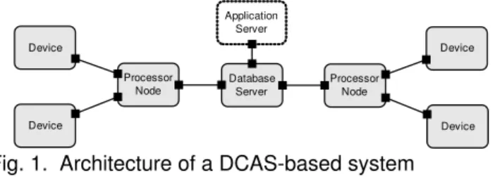
The basic building blocks in DCAS systems (Figure 13) are:

Application Server Database Server Processor Node Processor Node Device Device Device Device

Fig. 1. Architecture of a DCAS-based system

- Devices are equipped with one or more sensors to obtain

data from the application domain (e.g., wind towers, solar

panels). Each one of these sensors has an associated data

stream from which data can be read. There may be different

types of devices connected to the network, each type with its particular characteristics (e.g., protocols, type of data, etc.).

Each type of device has an associateddevice profilespecifying

the data polling rate and the expected value ranges for the data.

- Database serverstores the data collected from devices.

- Processor nodes pull data from the devices at a given

rate (configured in the device profile), and dispatch this data to the database server. Each processor node includes

a set of processes called Data Requester Processor Pollers

(DRPPs) responsible for retrieving data from the devices. The communication between the DRPPs and the devices is

2. http://solutions.criticalsoftware.com/products services/csems/

3. The component-and-connector diagram follows the style of the ACME architectural description language.

synchronous, so the DRPP remains blocked until the device responds to a request for data or a timeout expires. Note that this constitutes the main performance bottleneck of DCAS when devices connected to a processor node fail to respond in a timely manner.

- Application server is connected to the database server to obtain data, which can be presented to the operators of the system or processed automatically by application software. Since DCAS is application-agnostic, the application server will not be discussed in the remainder of this document.

The main objective of DCAS is collecting data from the connected devices at a rate as close as possible to the one configured in their device profiles, while making an efficient use of the computational resources in the processor nodes. Specifically, the primary concern in DCAS is providing service while maintaining acceptable levels of performance, measured in terms of processed data requests per second (rps) inserted in the database. The secondary concern is optimizing the computational cost of operating the system, measured in terms of active DRPPs in the processor nodes.

DCAS contains adaptation mechanisms aimed at maintain-ing its performance under different loads, respondmaintain-ing to failmaintain-ing devices, increased number of devices, and changing data rates:

- Rescheduling aims at avoiding performance degradation

caused by devices that fail to respond in a timely manner when polled. It consists in decreasing the priority of the data streams associated with the failing devices, so that they are polled less often (thus reducing the average time that DRPPs remain blocked waiting for device data).

- Scale upaims at improving system performance by exploit-ing as much as possible the resources (CPU and memory) of the processor nodes by (de)activating additional DRPPs as required. If the size of a request queue associated with a particular processor node remains consistently close to zero, scale up considers that there are active DRPPs that are not necessary and starts deactivating them (one at a time). Otherwise, if the queue size increases consistently, scale up tries to increase performance by activating more DRPPs.

DCAS has been chosen to evaluate our approach since: (i) it is a real system with a level of complexity representative of an industrial-scale software system, (ii) it has a well-defined set of objectives that enable the evaluation of resilience with respect to their fulfillment, and (iii) its implementation is available and amenable to evaluation in the context of a variety of changeload scenarios. Note that in its original version, DCAS is a legacy system that provides limited adaptation capabilities. However, in this paper we consider a MAPE-K-based version of DCAS that was re-engineered using Rainbow.

4

A

Our proposal for evaluating the resilience of a self-adaptive software system considers the model depicted in Figure 2.

The environment consists of all non-controllable elements

that determine the operating conditions of the system (e.g., hardware, network, physical context, etc.). We distinguish

two main subsystems in the self-adaptive system: a target

system, which is the subsystem to be controlled and which

may affect or be affected by its environment, and acontroller

that manages the target system, driving adaptation whenever it is required. The controller carries out its function by: (i)

monitoring the target system and environment throughprobes

that provide information about the value of relevant variables, (ii) deciding whether the current state of those variables demands adaptation, and if so, (iii) applying control actions

viaeffectors.

Self-Adaptive Software System Controller

Environment

Non-controllable software, hardware, network, physical context Target System Effectors Adapt Probes Monitor Monitor Affect Mo ni to r Probes Inputs Outputs

Fig. 2. Self-adaptive software system

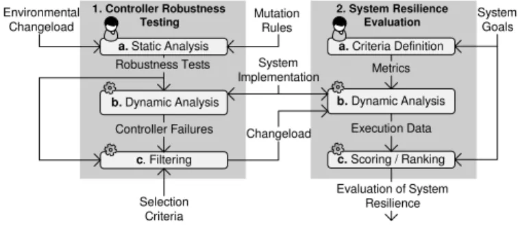
Our approach for evaluating robustness-driven resilience is intended to be used by the developer of the system just before its deployment, since the process often involves putting the system through adverse conditions which are not appropriate when the system is in production. The approach consists of

two phases, as shown in Figure 3 4_:

a. Static Analysis 1. Controller Robustness Testing 2. System Resilience Evaluation a.Criteria Definition b.Dynamic Analysis Metrics Evaluation of System Resilience c.Scoring / Ranking Execution Data c. Filtering Changeload Environmental Changeload Mutation Rules System Goals Selection Criteria System Implementation Robustness Tests b. Dynamic Analysis Controller Failures

Fig. 3. Overview of the approach

1) Controller Robustness Testing. In this phase, probe in-put (both from the target system and the environment) is modified to uncover potential controller failures. This

phase is divided into: (a) Static Analysis, in which the

engineer identifies the elements required to build the

ro-bustness test cases; (b) Dynamic Analysis, during which

controller robustness is tested. Uncovered controller failures

are categorized according to a failure mode classification;

and (c) Filtering, in which robustness test cases that did not uncover any failures in the controller are filtered out.

The output of filtering is a changeload including only the

scenarios that were not discarded.

2) System Resilience Evaluation. In this phase, the resilience of the system is evaluated according to the identified

changeload. This phase is divided into:(a) Criteria

Defini-tion, where resilience metrics are defined according to the

system goals (i.e., requirements);(b) Dynamic Analysis, in

which the system is stimulated according to the specification

4. Steps decorated with a gear in the figure are fully automatic, whereas steps decorated with the designer require input from the user.

of every scenario included in the changeload, and system execution traces are collected according to the metrics; and(c) Scoring/Ranking, where the collected information is processed and used to assess and rank the impact of the different controller failures in resilience. Every set of execution traces is aggregated into a probabilistic response model of the system. These models are used as input to a probabilistic model-checker, which quantifies the probabil-ities of satisfaction of the formalized resilience properties. Note that the first phase of our approach is intended as a single-run filter to identify scenarios that cause controller failures. In contrast, the second phase subjects the system to many runs of every scenario identified in the first phase to produce the probabilistic models for resilience evaluation.

In the following, we describe in more detail the key phases of our approach.

4.1 Controller Robustness Testing

The procedure for testing the robustness of the controller includes the following steps: (i) robustness tests used for stimulating the interface of the controller, (ii) controller failure mode classification, (iii) changeload model used to stimulate the system during resilience evaluation, and (iv) a description of the robustness testing procedure. These steps will be de-tailed in the subsequent subsections.

4.1.1 Robustness Tests

The basis of the proposed procedure for evaluating the robust-ness of controllers for self-adaptive software systems relies on stimulating the probes that monitor both the target system and its environment (see Figure 2). For evaluating how robust the controller is, the probes’ inputs into the controller are modified according to a comprehensive set of mutation rules.

It is important to emphasize that we do not have a priori

knowledge about the target fault model of the controller. Our mutation rules follow a fault model that has been shown to be relevant for the validation of input in the context of robustness testing [27], [28], [29].

Moreover, since the inputs of these probes may affect the different stages of a MAPE-K control loop, the testing procedure needs to consider the controller as stateful. Although we abstract away from the application (target system) during the robustness testing of the controller, we actually use the application to drive the tests (see Section 4.1.4 for details).

Mutation Rules. The robustness test cases are

automati-cally generated by applying predefined mutation rules to the messages sent by probes. The basic input supplied by probes to the controller requires three elements, although additional elements may exist depending on the case: (i) an identifier of the variable being monitored, (ii) the value for the variable, and (iii) a timestamp that provides a temporal context for the variable being monitored. For example, in the case of Rainbow, the input received by the controller consists of simple messages encoded as text strings with the format:

[ timestamp ] variable_name : variable_value

Based on this general description of probe inputs, we propose a set of rules (Table 1) for mutating the input from

Type Rule Name Description

Message

MsgNull Replace by null value MsgEmpty Replace by empty string MsgPredefined Replace by predefined string

MsgNonPrintable Replace by string with non-printable characters MsgAddNonPrintable Add non-printable characters to the string MsgOverflow Add characters to overflow max string size

T

imestamp

TSEmpty Replace by empty timestamp TSRemove Remove timestamp from response TSInvalidFormat Replace by timestamp with invalid format TSDateMaxRange Replace date in timestamp by maximum valid TSDateMinRange Replace date in timestamp by minimum valid TSDateMaxRangePlusOne Replace timestamp date by maximum valid +1 TSDateMinRangeMinusOne Replace timestamp date by minimum valid -1 TSDateAdd100 Add 100 years to date in timestamp TSDateSubtract100 Subtract 100 years from date in timestamp TSInvalidDate Replace date in timestamp by invalid date

V

ar

.

Name

VNRemove Remove variable name

VNSwap Replace by other variable name of same type VNSwapType Replace by variable name of different type VNInvalidFormat Replace by variable name with invalid format VNNotExist Replace by non-existing variable name

V

ar

.

V

alue

VVRemove Remove variable value

VVInvalidFormat Replace value by one with invalid format

Number VVNumAbsoluteMinusOne Replace by -1 VVNumAbsoluteOne Replace by 1 VVNumAbsoluteZero Replace by 0 VVNumAddOne Add 1 VVNumSubtractOne Subtract 1

VVNumMax Replace by maximum number valid for type VVNumMin Replace by minimum number valid for type VVNumMaxPlusOne Replace by maximum valid type value +1 VVNumMinMinusOne Replace by minimum valid type value -1 VVNumMaxRange Replace by maximum valid variable value VVNumMinRange Replace by minimum valid variable value VVNumMaxRangePlusOne Replace by maximum valid variable value +1 VVNumMinRangeMinusOne Replace by minimum valid variable value- 1

Boolean

VVBoolPredefined Replace by predefined value

TABLE 1

Mutation rules for probes

the probes [27], [28], [29]. The mutation rules target limit conditions that frequently represent difficult validation aspects, which are typically the source of robustness problems [27], [28], [29]. As an example, in [27] NULL and invalid pointer values were found to be quite common causes of failures. In our case, we consider faults that may be caused by the presence of some elements in the input, such as:

• Null and empty values (e.g., null string, empty string).

• Valid values with special characteristics (e.g., non-printable

characters in strings, dates by the end of the millennium).

• Invalid values with special characteristics (e.g., invalid dates

using different formats).

• Valid values equal to the maximum/minimum representative

of the domain.

• Values exceeding the maximum/minimum valid domain

values (e.g., maximum value valid for the parameter plus one).

• Values that cause data type overflow (e.g., string beyond

max size, duplicate list elements, maximum number valid for numeric type plus one).

In our approach, the values used for the parameters in mutation rules are static, and as such, we do not account for variance. This reduces the number of test cases, facilitating the developer’s task (it would be impossible to consider all input possibilities and combinations). In practice, we have a library of rules that define the possible parameters, along with the mutations. Previous experience suggests that this simple setup is enough to trigger problematic behaviors in many systems

[29], [35]. Although the analysis of variable values may be useful in disclosing other failures, the focus of this paper is not about the actual application of robustness testing technique to uncover failures, but on the development of an approach for evaluating the resilience of self-adaptive systems that relies on the outcome of applying robustness testing principles.

Probe Categories. The effect of applying mutation rules on the input received from the probes may manifest in different ways (or not manifest at all) in the controller, depending on its internal state. This results from the stateful nature of the controller, which may use different inputs and in a different way, depending on its operational stage (i.e., analysis, planning, or execution).

Table 2 shows different probe categories, according to their use in the different operational stages of the controller. Dif-ferent robustness issues may arise in the controller, depending on the particular stage and probe in which a mutation rule is applied. The same probe may belong to different categories and be used during different stages in the controller. We currently consider a coarse-grained notion of controller state that corresponds to each of the operational stages of the controller. As a simplification, we assume each stage to be stateless. This enables the evaluation of resilience considering the stateful nature of MAPE-K controllers, even in cases in which we do not have access to the internals of the different stages. However, future work will consider a finer-grained notion of state, considering other elements (e.g., control flow of adaptation logic in the controller execution stage) as part of controller state.

4.1.2 Controller Failure Modes

The robustness of a controller for a self-adaptive system can be classified according to a modified version of the CRASH scale [27], which distinguishes the following failure modes:

(1) Catastrophic: the whole controller crashes or becomes

corrupted (this might include the OS or machine on which

the controller is running). No output is produced;(2) Restart:

the controller execution hangs and may not issue any output commands, or send always the same command, within the worst case execution time of the adaptation cycle. The

con-troller needs to be externally re-booted; (3) Abort: abnormal

behavior by the controller occurs due to a run-time exception

raised inside the controller; (4) Silent: the controller fails to

acknowledge an error, for instance by signalling an exception, which causes the controller to continue operating improperly;

(5) Hindering:the controller returns an incorrect error code, which may hinder error recovery.

Different from the original CRASH scale [27], our tailored version includes a specific adaptation which is related to time (2).

4.1.3 Changeload Model

This section describes the proposed changeload model

(adapted from [21]) and presents the definition of its

fun-damental concepts:

Definition 1 (Change Type): A change type is a tuple

(src,m,A) that characterises a change, where: src identifies

the source probe type mutated, midentifies the mutation rule

applied, and A=ha1, . . . ,ani (possibly empty) is a vector of

attributes holding information about the mutation rule.

Example 1: In DCAS, consider the change “Set an invalid

timestamp date on a queue size probe (typeQueueSizeProbeT)”.

A possible change type definition for this would be:

invalidDateQSP CT=(QueueSizeProbeT,TSInvalidDate,hdatei)

Definition 2 (Change): Given a set of change types CT, a

change is a tuple (ct,srcinst,VA,ti,d) that corresponds to an

instantiation of a change type, where: ct =(src,m,A)∈ CT

determines the change type to be instanced as a change,

srcinst is the probe instance that is the source of change,

VA =hvA1, . . . ,vAni is a vector of attribute values instantiating

the attributes in A, ti ∈ _R+₀ is the time instant in which the

change is triggered, andd∈_R+is the change duration.

Example 2: If we consider the change type described in

Example 1, a possible instantiation could be:

(invalidDateQSP CT,QueueSizeProbe1,h0_2/29/19850_i,10,2)

The systematic identification and classification of change types is fundamental to support the definition of change scenarios, which is discussed in the next paragraphs.

The main concept in our changeload model is that of a scenario. A scenario is a postulated sequence of events that captures the state of the system and its environment, system

goals5_{, and changes affecting all the aforementioned elements.}

It is defined in terms of state (target system and environment) and changes applied to that state.

Definition 3 (Scenario): A scenario is a tuple (wl,oc,C)

where: wl represents the workload, that is, the amount of

work assigned to the system (not necessarily static), oc are

the operational conditions of the system, and C is a set of

changes applied to controller input.

Based on the definition above, a change scenario is one

which includes a non-empty set of changes (C,∅).

Definition 4 (Changeload): Set of change scenarios.

4.1.4 Robustness Testing Procedure

Robustness testing focuses on the controller’s input delivered by probes. Therefore, a complete robustness experiment must include a comprehensive set of robustness tests including on the information provided by each of the input probes used during each of the different operational stages of the controller. The procedure for robustness testing consists of three steps:

Static Analysis. This step is carried out manually by the

engineer, and consists in identifying: (i) the conditions of the environment required to drive the controller through its

dif-ferent operational stages (environmental changeload)6; (ii) the

set of probes used during each controller stage; and (iii) the set of mutation rules applicable to each of the probe inputs used in the different controller stages.

Example 3: Consider a setup of a DCAS system that

processes a constant workload which includes 100 devices with a sample rate of 1 second each:

5. However, in our approach we assume a changeload model that does not consider changes in system goals.

6. These conditions can be identified based on the engineer’s domain knowledge, the analysis of similar systems, or through a systematic analysis of the possible changes in the environment and their impact on the controller’s behavior [8].

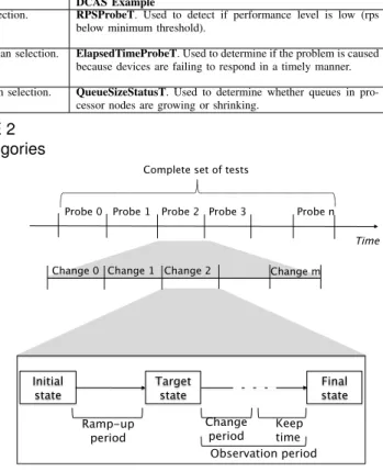
Probe Category Controller Stage Input Usage DCAS Example

Analysis The controller analyzes the current state of the target system for detecting anomalies, and triggering adaptation if needed.

Anomaly detection. RPSProbeT. Used to detect if performance level is low (rps below minimum threshold).

Planning The controller determines if any adaptation plans can be applied to the target system, and selects the best alternative.

Adaptation plan selection. ElapsedTimeProbeT. Used to determine if the problem is caused because devices are failing to respond in a timely manner.

Execution The controller executes the selected course of action. Control action selection. QueueSizeStatusT. Used to determine whether queues in pro-cessor nodes are growing or shrinking.

TABLE 2 Probe categories

• Environment conditions. With a constant workload, the

con-ditions of the environment required to drive the controller through its different operational stages in DCAS are related to the time that it takes for devices to respond to data requests. Driving the controller through its planning and execution stages involves artificially inducing a 2-second delay to 25% of device responses. In this case, this in-formation has been determined experimentally during prior deployments of DCAS in the field [32].

• Probes used and applicable mutation rules. Inspecting the

implementation of the target system, the different sets of probe types used in each of the controller’s operational stages are identified. For each of the identified probes, we determine which of the mutation rules are applicable to generate the robustness test cases.

Probe Type Applicable mutation rules

Analysis Planning Execution

RPSProbeT 30 x x QueueSizeProbeT 31 x x x QueueStatusProbeT 29 x ActivePollersProbeT 31 x ElapsedTimeProbeT 31 x x TABLE 3

DCAS probes and applicable mutation rules

Table 3 displays the results of this identification process in DCAS. Each applicable mutation rule yields a different robustness test case for each controller stage in which the probe is used. In this case, we have a total of 275 robustness tests to carry out for assessing the robustness of the controller

(30 rules * 2 stages for RPSProbeT + 31 rules * 3 stages for

QueueSizeProbeT + 29 rules * 1 stage for QueueStatusProbeT + 31

rules * 1 stage for ActivePollersProbeT + 31 rules * 2 stages for

ElapsedTimeProbeT).

Dynamic Analysis. During this step, the controller’s robust-ness is tested according to the test cases identified in the previous step. Figure 4 shows that this step includes several subsets of tests, each one focusing on one probe. For each probe (which, at run-time is continually delivering information to the controller), we run a robustness test that applies a single

change to each probe data sample. Note that although we

apply a single change to a data sample produced by a probe, the same change is applied to all subsequent samples received within the time period defined by the duration of the change (see Definition 2).

Each robustness test focuses on a single mutation rule type, and is executed once in every controller operational stage to maximize the chances of disclosing more robustness problems. In each test, we must drive the system from an initial state to a target state by stimulating it according to a change scenario

t1 – Rampup (changeload execution)

t2 – Fault injection (while still on the target state. What is the limit for fault injection if there is no state transition? Number of faults, time,?)

t3 - Keep time (time to reach the end of a cycle (may not be reached, will need to be fit in the failure modes) t4 – Observation period

Target state: The initial state for testing

Target state: The state we want to drive the system to start testing Final state: Should be the end-of-cycle state, but is eventually unknown

state in the diagram is related to the state of the experiment – in our case we can only observer in which stage the controller is Keep time Observation period Change period Ramp-up period Probe 3

Probe 0 Probe 1

Time

Complete set of tests

Change 0Change 1

it is not a black-box, it is grey-box;

the final state is the end of the cycle, end of execution and we can observe the consequences; several faults of a single type

single fault versus multiple faults of the same type

determine the number of faults through experimentation (representativeness), period should be based on the controller response time or cycle – length of the experiment

(worst case execution time from the srategy) Initial

state Target state Final state

Fig. 4. Robustness testing procedure

during a ramp-up period (Figure 4). This target state is the

one in which the system must be to start testing, and can correspond to the entry point to any of the three controller stages. With the controller in the target stage, we can start

applying the changes (of the same type7_{) for achange period}

during which the controller is on the target stage for the test. This period of time should be adjusted to the time required to transition from the target controller stage for the test to the next stage.

After this probe mutation period, there is a keep time

required for the system to reach a final state that marks the end of the current test (and corresponds to the completion of the controller’s execution stage). At most, the keep time should be set to the worst case execution duration found in the

specification of the adaptation to be executed. Theobservation

period (change+keep time periods) is used to register any

deviations from expected controller behavior.

Filtering. Consists in reducing the number of test cases by discarding the robustness tests that did not meet the selection criteria (i.e., that did not uncover failures in the controller). Note that the selection criteria can be tailored to different situations (e.g., by selecting tests that uncovered controller failures only in a constrained set of categories of our adapted CRASH scale).

In our study, we identify controller failures via inspection

7. We could have considered combinations of different types of change during this period, instead of a single type. However, the number of combi-nations can become quite large and we chose to follow the usual procedure in robustness testing. Even using a single type of change, we were able to uncover a considerable number of controller failures during the evaluation of the approach (see Section 5).

of the execution logs produced by Rainbow. Silent failures correspond to incorrect updates of property values in the ar-chitecture models that are not acknowledged by the controller (e.g., updating the a response time property with a negative value). Due to the subtle nature of some of these failures, log inspection is carried out manually to discriminate silent failures from fault masking, for example. Fault masking can occur in Rainbow during pre-filtering of the input received from probes. This is carried out by gauge components con-nected to the controller, which are in charge of updating the architecture model.

4.2 System Resilience Evaluation

In the previous subsection we described controller robustness testing, aimed at obtaining a changeload that induces failures in the controller. In this subsection, we: (i) introduce some general concepts related to resilience evaluation, as well as the kind of resilience properties that we deal with and their formalization, and (ii) describe the procedure followed for resilience evaluation of the system in the presence of failures in the controller.

4.2.1 Resilience Properties

A resilient system is one that delivers a service that can

justifiably be trusted when facing changes[3]. In the context of

self-adaptive systems, changes (which can occur in the system itself, its environment, or goals) can induce anomalies in the

system at run-time, changing its current operational profile.

Specifically, within a self-adaptive system we may distinguish

between a conventional operational profile (COP) that

corre-sponds to the region of the state-space in which the system

is operating without experiencing any anomalies, and

non-conventional operational profiles (NCOPs), associated with

changes that induce anomalies in the system and correspond to regions of the state-space in which the system is experiencing a particular anomaly. When the self-adaptive system enters a NCOP, this typically triggers adaptation mechanisms whose purpose is driving the system back into its COP by perform-ing some actions on the system to correct the experienced anomaly. The system behavior in different operational profiles is represented in our approach by means of DTMCs built over relevant variables monitored during execution, and are

obtained via synthesis from system traces8 _[7].

For evaluating the resilience of a self-adaptive system, two cases need to be considered according to its operational profile: (i) when there is a change while the system is in its COP, resilience can be assessed by quantifying the probability of not transitioning into a NCOP within a certain time interval, and (ii) when the system is already in a NCOP, resilience can be assessed by quantifying the probability of returning into the COP within a certain time interval.

To express resilience properties about the system, we use PCTL [6], which is a temporal logic language that can be used to express system properties that are domain-dependent. Fur-thermore, to ease the formulation of probabilistic properties, we use property specification patterns that describe generalized recurring properties in probabilistic temporal logics. Since we

8. See Appendix A for DTMC-based definitions of operational profiles.

PCTL Formulation Description

P≥1[G(Φ1⇒ P./p(F≤tΦ2))] Probabilistic Response.After state for-mula Φ1 holds, state formula Φ2 must becometruewithin time boundt, with a probability bound./p.

P≥1[G(Φ1⇒ P./p(¬Φ2U≤tΦ3))] Probabilistic Constrained Response. Af-ter state formulaΦ1holds, state formula Φ3must become true, withoutΦ2 ever holding, within time boundt, with a prob-ability bound./p.

TABLE 4

Probabilistic response specification patterns

are interested in how the system responds to changes, we focus on properties that can be instanced by using probabilistic

response patterns [34], adapted to PCTL syntax (see Table 4).9

These patterns include a premiseΦ1 that represents the initial

conditions after a change in the system or its environment occurs. They also include a subformula enclosed by the

probabilisic operator P_./p(.), representing the response to that

change expected from the system (with a probability bound p

and a time boundt).

Example 4: In DCAS, we are interested in assessing how

the system reacts to low responsiveness in some of the devices

connected to the system. Let rpsbe the variable associated

with performance (defined as the number of items inserted in

the database per second), and numActivePollersbe the variable

associated with operating cost (defined as the number of active pollers in the system). We can then define the following predicates:

rpsViolation=rps<MIN RPS hiCost=numActivePollers≥MAX POLLERS

whereMIN RPSis a threshold that establishes the minimum

ac-ceptable performance of the system, andMAX POLLERSdetermines

a maximum acceptable number of active pollers. Let us also express a predicate associated with the COP in DCAS as

dcasCOP=¬rpsViolation∧¬hiCost. Based on these predicates, we

may instantiate the following PCTL properties, making use of the probabilistic response pattern included in Table 4:

P1:P_≥1[G(dcasCOP⇒ P_≤0.2(F≤100 rpsViolation))]

P2:P≥1[G(rpsViolation⇒ P≥0.9(F≤100¬rpsViolation))]

P1 deals with the first resilience evaluation case described above (COP), and reads as: “When operating with acceptable performance and cost, the probability of performance dropping

below MIN RPSwithin 100 seconds is less or equal to 0.2”. In

contrast, P2 deals with the second evaluation case (NCOP),

and reads as: “When performance falls below thresholdMIN RPS,

the probability of raising performance again above MIN RPS

within 100 seconds is greater or equal to 0.9”. Note that the probabilistic response patterns, as well as the predicates used for the specification of the properties can be more general or specific, depending on the particular aspect of the system

resilience that we want to study (e.g., use of ¬ rpsViolation

instead ofdcasCOPin P2).

4.2.2 Resilience Evaluation Procedure

System resilience evaluation consists in exercising the target

9. Although this paper focuses on probabilistic response patterns to express resilience properties, nothing prevents the use of the proposed approach with other patterns to study different classes of system properties.

A. Conventional Operational Profile (Analysis)

Run 0

(baseline )

Run 1 Run 2 Run 3 Run n

time measurement interval keep time check time steady state condition stop condition steady state time time to adapt start of adaptation

probe mutation period (analysis )

B1. Non-Conventional Operational Profile (Planning)

Run 0

(baseline )

Run 1 Run 2 Run 3 Run n

time measurement interval environment stimulation time to react time to adapt keep time check time steady state condition adaptation trigger condition stop condition steady state time start of adaptation probe mutation period (planning )

B2. Non-Conventional Operational Profile (Execution)

Run 0

(baseline )

Run 1 Run 2 Run 3 Run n

time measurement interval environment stimulation time to react time to adapt keep time check time steady state condition adaptation trigger condition stop condition steady state time start of adaptation probe mutation period (execution )

Guaranteed condition / event Uncertain condition / event

Fig. 5. Dynamic analysis: COP (top) and NCOP (bottom)

system (and its environment) using the identified changeload to assess the resilience of the system in the presence of the controller failures identified during robustness testing. It includes the following steps:

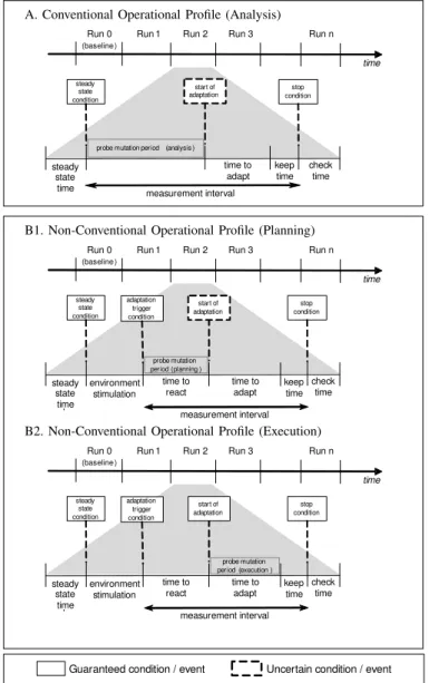
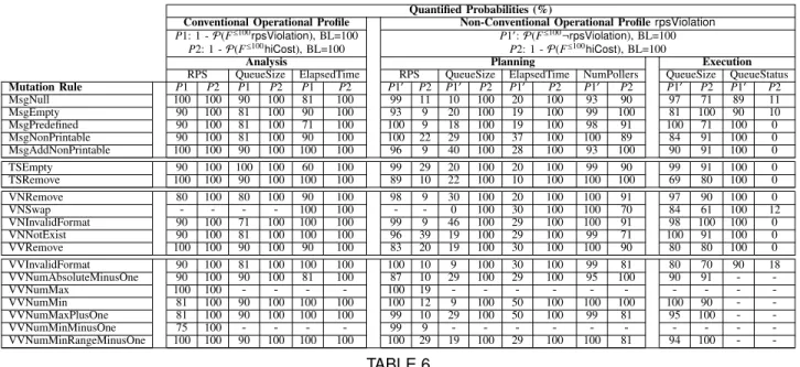
Criteria Definition. The definition of resilience incorporates the fulfillment of system goals. Hence, the criteria for as-sessment (i.e., the metrics) must be defined according to the system’s goals, since we want to understand how effective the system is at satisfying them in the presence of controller failures. In DCAS, the system needs to maximize performance while maintaining a low operation cost. These requirements are reflected on the resilience properties (formally expressed in the PCTL formulas shown in Table 6).

Dynamic Analysis. The analysis can be divided into two

cases (see Figure 5), which establishes the profile of the resilience experiments. This partition is made according to the target system’s operational conditions. The assessment of every operational case (NCOP or COP) includes a set of test runs, where Run 0 is a baseline run that includes no probe mutations. This baseline run is used later as a reference to understand the impact of the filtered probe mutations (i.e.,

mutations that resulted in controller failures, as observed in the previous phase) in the overall system resilience. The self-adaptive system state must be explicitly restored in the beginning of each run so that the effects of the tests do not accumulate across different runs.

Figure 5.A reflects the case where we assess the target system when there is no need for adaptation (i.e., the system is running in a conventional operational profile). Figure 5.B1 and 5.B2 represent the case where the goal is to assess the target system when it is running in a non-conventional operational profile (i.e., adaptation is required).

Regarding the conventional operational profile case (Fig-ure 5.A), the following steps are carried out. The target system must reach a steady state condition (steady state time). After this condition is met, we apply probe mutations using the filtered changeload mentioned earlier, which may result in triggering adaptation or not. Note that adaptation may be triggered as a consequence of the probe mutations, and not due to the state of the target system. If triggered, we stop applying mutations and observe the system behavior during the adaptation process (i.e., during time to adapt) and after adaptation is concluded for a given amount of time (keep time in Figure 5.A). A period used to let the system stabilize again finishes the execution of the system (i.e., check time). If adaptation does not start during a test, probe mutation continues until the stop condition is met.

The non-conventional operational profile case requires trig-gering adaptation. We consider two subcases that differ in the probe mutation period, which is carried out when the controller is in two distinct stages: planning and execution, which are shown, respectively, in Figure 5.B1 and 5.B2. In subcase B1, probes are mutated immediately after the adaptation trigger condition is met and until adaptation starts. The remaining periods serve the same purpose as in Figure 5.A. If adaptation does not start (e.g., as a consequence of probe mutation), mu-tation continues until the stop condition is met. In subcase B2, probe mutation begins after adaptation starts and is executed during the time required to adapt until the keep time is reached.

Scoring/Ranking. Finally, the collected data (execution

traces) is used to rank the impact on resilience of the different controller failures, considering the criteria previously defined. In practice, the set of traces collected during the execution of each change scenario is aggregated into a probabilistic response model of the system. These models are used as input to a probabilistic model-checker, along with the resilience properties obtained from system goals. As an outcome, re-silience can be evaluated using the quantified value of the probability of satisfaction for the resilience properties obtained from the model-checker.

5

E

In this section, we assess the validity of our approach by testing the robustness of a DCAS controller developed using Rainbow (i.e., a tailored version of Rainbow’s master con-troller) and evaluating the resilience of the implementation of the DCAS system described in Section 3.

In the following, we first provide a brief overview of Rainbow, followed by a description of the setup employed for our evaluation, and results.

5.1 The Rainbow Framework

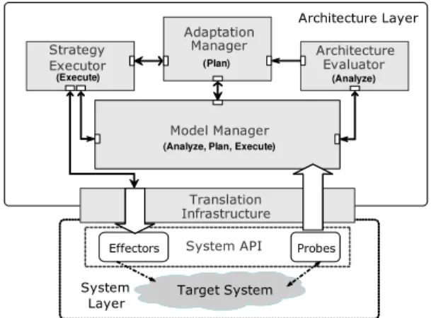
The focus of this paper is on a controller built using Rain-bow [9], an architecture-based platform for self-adaptation. This platform provides a substantial base infrastructure that can be customized, and has the following distinctive features: an explicit architecture model of the target system, a collection of adaptation strategies, and utility preferences to guide the adaptation process.

The Rainbow framework includes mechanisms for (see Figure 6): monitoring a target system and its environment (the observations are used to update the architecture model of the target system and its environment), detecting opportunities for improving the system’s quality of services (QoS), deciding the best course of adaptation based on the state of the system, and effecting the most appropriate changes. Rainbow’s component-and-connector architecture model of the target system is one of the main elements supporting self-adaptation. It is used to reflect monitored target system and environment information, and to reason about appropriate adaptation mechanisms for a particular situation.

The main components of the framework are:

• Architecture Evaluator:evaluates the model to ensure that

the system is operating without experiencing any anomalies (e.g., violation of an invariant). If an anomaly is detected, adaptation is triggered.

• Adaptation Manager:chooses a suitable strategy based on

the current system and environment state (reflected in the architecture model).

• Strategy Executor: executes the strategy chosen by the

adaptation manager via system-level effectors.

• Model Manager:updates the architecture model using the

information collected from the system and its environment via probes. System Layer Architecture Layer Target System Target System Translation Infrastructure Adaptation Manager Model Manager Strategy Executor

System API Probes Effectors Architecture Evaluator (Analyze) (Plan) (Execute)

(Analyze, Plan, Execute)

Fig. 6. The Rainbow framework

5.2 Setup

We deployed a Rainbow-based controller and DCAS across

four machines (Figure 7):dcas-dbacts as the backend database

running on Oracle 10.2.0, dcas-main acts as a processor node,

running DCAS, anddcas-devsis used to simulate the response

of network devices from which DCAS retrieves information.

The controller (Rainbow’s master) is deployed indcas-master.

All machines have anIntel core i3processor, 1GB of RAM, and

runWindows XP Pro SP3 (DCAS runs as a Windows service).

dcas-main

dcas-db dcas-devs

dcas -master

Fig. 7. DCAS experimental setup

To build the changeload for our evaluation, we identified the: (i) workload and operating conditions for change scenarios characteristic of a typical deployment of a DCAS system in production, (ii) set of probes used during the analysis, planning, and execution stages of the controller (Table 3), and (iii) set of changes to be applied on our set of probes, which was determined by identifying the applicable mutation rules for each probe (Table 3).

Concening the workload and operating conditions employed in our study, they have been scaled down to a duration of 5 minutes (300s), which is enough to: (i) drive the con-troller through its different operational stages and apply the robustness tests, and (ii) collect enough data to synthesize the probabilistic models required to quantify the system’s resilience. The workload employed in all scenarios includes 100 data streams with a sample rate of 1 second. We carried out two types of evaluation: (i) COP, which uses the regular workload and normal operating conditions (no unresponsive devices) throughout the entire duration of the experiment (300s), and (ii) NCOP, in which the controller is driven towards triggering adaptation to improve performance, and that conforms to the following pattern: (a) 50s of normal activity to let the system achieve a steady state; (b) 200s during which we induce low responsiveness in devices (adding a 2-second delay in the response time of 25% of the data streams); and (c) 50s of normal activity.

5.3 Results

In this subsection, we present the results of: (i) controller robustness testing, and (ii) system resilience evaluation in the presence of controller failures.

5.3.1 Controller Robustness Testing

Each change scenario of the changeload results from com-bining the workload and operating conditions with a change related to an applicable mutation rule. For each mutation rule, we generate one scenario per probe per controller stage. Overall, we run 275 robustness tests (the number of tests run is justified in Example 3, and each test was repeated 3 times to confirm the results).

Table 5 details the results obtained. When mutating the inputs from the probes, the columns in the table show the number of silent (S) and abort (A) failures related to the stage of the controller, and the probes associated to that stage. To begin with, 152 out of the 275 conducted tests uncovered

Failures (A=Abort, S=Silent)

Analysis Planning Execution

RPS QueueSize ElapsedTime RPS QueueSize ElapsedTime ActivePollers QueueSize QueueStatus

Mutation Rule A S A S A S A S A S A S A S A S A S MsgNull 1 1 1 1 1 1 1 1 1 1 1 1 1 1 1 1 1 1 MsgEmpty 1 1 1 1 1 1 1 1 1 MsgPredefined 1 1 1 1 1 1 1 1 1 MsgNonPrintable 1 1 1 1 1 1 1 1 1 MsgAddNonPrintable 1 1 1 1 1 1 1 1 1 TSEmpty 1 1 1 1 1 1 1 1 1 TSRemove 1 1 1 1 1 1 1 1 1 VNRemove 1 1 1 1 1 1 1 1 1 VNSwap 1 1 1 1 1 1 VNInvalidFormat 1 1 1 1 1 1 1 1 1 VNNotExist 1 1 1 1 1 1 1 1 1 VVRemove 1 1 1 1 1 1 1 1 1 VVInvalidFormat 1 1 1 1 1 1 1 1 1 VVNumAbsoluteMinusOne 1 1 1 1 1 1 1 1 VVNumMax 1 1 VVNumMin 1 1 1 1 1 1 1 1 VVNumMaxPlusOne 1 1 1 1 1 1 1 1 VVNumMinMinusOne 1 1 VVNumMinRangeMinusOne 1 1 1 1 1 1 1 1 TOTAL/PROBE 1 18 1 16 1 17 1 18 1 17 17 1 17 1 17 1 13 TOTAL/STAGE A: 3, S: 51 A: 4, S: 69 A: 2, S: 40 TABLE 5

Experimental results for controller robustness testing

robustness issues (55%). Moreover, no catastrophic, restart, or

hindering failures were identified during the tests10_.

Regard-ing abort failures, only tests related to the mutation MsgNull

uncovered a single failure per probe and in all controller stages. This failure is consistent with the same unhandled

java.lang.NullPointerException raised during the parsing of probe response using a regular expression matcher.

Silent failures are by far the most frequent failure type discovered during the tests. Mutations that affect the overall probe response message, as well as the variable name and value (first, third, and fourth groups in Table 5, respectively) present the highest concentration of silent failures. In contrast, silent failures that concern timestamps occurred only in cases

in which such element is removed (mutations TSEmpty and

TSRemove). A detailed analysis showed that this is a conse-quence of the way in which Rainbow’s controller processes inputs from the probes. Messages are parsed in such a way that only the presence of a timestamp in the message is assessed, but its value is not checked syntactically nor semantically. However, this does not prevent the correct update of values in the architectural model of the system inside of the controller in spite of incorrect timestamps in probe input. Moreover, all the observed silent failures correspond to incorrect updates of values in the architectural model, which are not acknowledged

by the controller in any way. It is worth mentioning thatsilent

failures discovered in the different controller stages are different. For example, we observed that in some situations, properties in the architecture model are updated with the

null value in tests conducted during the analysis stage. In

contrast, in the planning and execution stages the value of the architecture property stops being updated when the same mutation rule is applied on the same probe. This can lead to completely different behaviors of the controller that can affect the target system in different ways.

10. Despite this, these failure modes portray relevant behaviors that might be uncovered when testing other controllers.

5.3.2 System Resilience Evaluation

In line with the system’s objectives of maintaining an ac-ceptable performance level while keeping down the cost of running the system, we study the resilience of the system in the presence of the different controller failures observed during controller robustness testing. To achieve our goal, we built a set of probabilistic models from all the scenarios that

uncovered controller failures using a time frame [0,150], a

time sampling parameter (as described in Appendix A) of

τ=1s, and quantization parameters for performance and cost

ηrps = 10 and ηnumActivePollers = 1, respectively. Each model

is synthesized from data obtained from 30 different runs of the same scenario (i.e., including the 2 baseline models, our study required (2+152)*30=4680 runs). Using these models,

we quantify the levels of system resilience11 (Table 6) while

the system is in:

Conventional Operational Profile. The system is operating

steadily with good levels of performance and within cost, so adaptation is not required and the controller is in its analysis stage. We analyze resilience in terms of whether controller failures induce the target system to deviate from its COP (e.g., by triggering unnecessary adaptations). Deviation from the system’s COP can be either in terms of performance or cost. We quantify: (P1) the probability of performance level falling

below theMIN RPSthreshold by 100s (1-P(F≤100rpsViolation)),

and (P2) the probability of the number of active pollers

raising above the acceptable limit MAX POLLERS by 100s

(1-P(F≤100hiCost)). Probability values displayed in the Table 6

for P1 and P2 are complementary, so that higher values

indicate better resilience.

Non-Conventional Operational Profile. Associated with

anomalyrpsViolation. The system is underperforming, so

adap-tation has been triggered and the controller is in its planning or

11. Specifically, we show the results obtained from applying the probabilis-tic quantifierP(.) to system response according to the probabilistic response pattern displayed in Table 4. Implicit premises are dcasCOPfor the COP section, andrpsViolationfor the NCOP section.

Quantified Probabilities (%)

Conventional Operational Profile Non-Conventional Operational ProfilerpsViolation

P1: 1 -P(F≤100_{rpsViolation), BL=100 P1}0_:P(F≤100_{¬rpsViolation), BL=100} P2: 1 -P(F≤100_{hiCost), BL=100 P2: 1 -P(F}≤100_{hiCost), BL=100}

Analysis Planning Execution

RPS QueueSize ElapsedTime RPS QueueSize ElapsedTime NumPollers QueueSize QueueStatus

Mutation Rule P1 P2 P1 P2 P1 P2 P10 _{P2 P1}0 _{P2 P1}0 _{P2 P1}0 _{P2 P1}0 _{P2 P1}0 _P2 MsgNull 100 100 90 100 81 100 99 11 10 100 20 100 93 90 97 71 89 11 MsgEmpty 90 100 81 100 90 100 93 9 20 100 19 100 99 100 81 100 90 10 MsgPredefined 90 100 81 100 71 100 100 9 18 100 19 100 98 91 100 71 100 0 MsgNonPrintable 90 100 81 100 90 100 100 22 29 100 37 100 100 89 84 91 100 0 MsgAddNonPrintable 100 100 90 100 100 100 96 9 40 100 28 100 93 100 90 91 100 0 TSEmpty 90 100 100 100 60 100 99 29 20 100 20 100 99 90 99 91 100 0 TSRemove 100 100 90 100 100 100 89 10 22 100 10 100 100 100 69 80 100 0 VNRemove 80 100 80 100 90 100 98 9 30 100 20 100 100 91 97 90 100 0 VNSwap - - - - 100 100 - - 0 100 30 100 100 70 84 61 100 12 VNInvalidFormat 90 100 71 100 100 100 99 9 46 100 29 100 100 91 98 100 100 0 VNNotExist 90 100 81 100 100 100 96 39 19 100 29 100 99 71 100 91 100 0 VVRemove 100 100 90 100 90 100 83 20 19 100 30 100 100 90 80 80 100 0 VVInvalidFormat 90 100 81 100 100 100 100 10 9 100 30 100 99 81 80 70 90 18 VVNumAbsoluteMinusOne 90 100 90 100 81 100 87 10 29 100 29 100 95 100 90 91 - -VVNumMax 100 100 - - - - 100 19 - - - -VVNumMin 81 100 90 100 100 100 100 12 9 100 50 100 100 100 100 90 - -VVNumMaxPlusOne 81 100 90 100 100 100 99 10 29 100 50 100 99 81 95 100 - -VVNumMinMinusOne 75 100 - - - - 99 9 - - - -VVNumMinRangeMinusOne 100 100 90 100 100 100 100 29 19 100 29 100 100 81 94 100 - -TABLE 6

Experimental results for system resilience evaluation

execution stage. We analyze resilience in terms of whether the system can return to its COP by a given deadline. We quantify:

(P10) the probability of the performance level raising above the

MIN RPSthreshold by 100s (P(F≤100¬rpsViolation)), and (P2),

as defined above. Higher values of both P10 and P2 indicate

better resilience.

Note that, the values labelled as BLin each section header

indicate the baseline value for the probability (i.e., the value obtained when no mutations are performed on the probes).

Table 6 displays predominantly high values, which indicate a high level of system resilience to controller failures. If we focus on the system’s COP, failures occurring in the controller during the analysis stage have a moderate effect on performance (P1 between 80-90% in all probes) and no effect on cost (P2=100% in all cases).

In contrast, if we focus in the NCOP part of the table, the

values in performance-related property P10 _{plummet in the}

presence of failures caused by mutations in QueueSizeProbeT

(10-46%) andElapsedTimeProbeT(10-50%) during the planning

stage. This lack of performance is encompassed by low levels of active pollers, as indicated by the corresponding values

of cost-related propertyP2. Although the remaining mutation

cases (RPSProbeTandNumPollersProbeT) in the planning stage

still maintain high performance levels (P10between 83-100%),

the values in P2 are affected, falling down to levels as low

as 9% for RPSProbeTwith mutation VNRemove. These figures

show that two failures in the same category may have

very different impacts on resilience.This is consistent with the fact that different probes provide information to update different properties of the architecture model that may be employed by the controller in disparate ways. Finally, the values in the execution stage indicate that performance and

cost are only moderately affected in QueueSizeProbeT (ranges

between 69-100% and 61-100% for P10andP2, respectively).

However, performance levels in QueueStatusProbeTare always

very high (P10, 89-100%), at the expense of remarkable drops

in the values of P2 (0-18%) due to high poller activation.

Finally, two failures in the same category may have

very different impacts on resilience, depending on the operational stage of the controller.For example, failures

in-duced in the controller by mutations inQueueSizeProbeTin the

planning stage indicate a remarkable impact in performance

P10_{, compared to the execution stage.}

6

L

Robustness testing is used at the interface of a system, and it essentially consists of providing invalid inputs with the goal of disclosing problems (by observing the output). In the case of our approach, we do not simply observe failures in the system where the fault is introduced. We inject mutations at one point (i.e., the interface of the controller), and observe their influence in another system (composed by the controller and the system being managed, i.e., the target system). The approach also considers the presence of a MAPE-K control loop (it perceives the controller as stateful), and as such, it is tailored to consider that the controller might be in different stages (which represent different states). Furthermore, the robustness tests are used to quantify resilience, since we are collecting resilience metrics from a robustness evaluation procedure. All of these are key aspects that make our approach diverge from the classic robustness testing scenarios to fit the specificities of self-adaptive systems. To the best of our knowledge, there is no other approach in the literature with these characteristics that could be used as a reference for comparative purposes.

Our approach constitutes a first step in exploring the impact on system resilience of controller failures, and is currently limited in a number of ways, as discussed next.

First, the work is limited to a subset of undesirable behaviors in adaptive systems, dealing only with controller failure cases resulting from malformed inputs. This leaves out other causes of controller misbehavior, such as flaws in the adaptation logic. Some of these cases (e.g., failure in executing adaptive actions in the target system) were explored in [8].