This is the author’s final, peer-reviewed manuscript as accepted for publication. The publisher-formatted version may be available through the publisher’s web site or your institution’s library.
This item was retrieved from the K-State Research Exchange (K-REx), the institutional repository of Kansas State University. K-REx is available at http://krex.ksu.edu
Bayesian mixture labeling and clustering
Weixin YaoHow to cite this manuscript
If you make reference to this version of the manuscript, use the following information: Yao, W. (2012). Bayesian mixture labeling and clustering. Retrieved from
http://krex.ksu.edu
Published Version Information
Citation: Yao, W. (2012). Bayesian mixture labeling and clustering. Communications in Statistics—Theory and Methods, 41(3), 403-421.
Copyright: © Taylor & Francis Group, LLC
Digital Object Identifier (DOI): doi:10.1080/03610926.2010.526741
Bayesian Mixture Labeling and Clustering
Weixin Yao
Department of Statistics, Kansas State University, Manhattan, Kansas 66506, U.S.A.
Abstract
Label switching is one of the fundamental issues for Bayesian mixture modeling. It occurs due to the nonidentifiability of the components under symmetric priors. Without solving the label switching, the ergodic averages of component specific quantities will be identical and thus useless for inference relating to individual components, such as the posterior means, predictive component densities, and marginal classification probabilities. In this article, we establish the equivalence between the labeling and clustering and propose two simple clustering criteria to solve the label switching. The first method can be considered as an extension of K-means clustering. The second method is to find the labels by minimizing the volume of labeled samples and this method is invariant to the scale transformation of the parameters. Using a simulation example and two real data sets application, we demonstrate the success of our new methods in dealing with the label switching problem.
Key words: Bayesian mixtures; Clustering; K-means; Label switching; Markov chain Monte Carlo;
1
Introduction
Supposex= (x1, . . . , xn) are independent observations from am-component mixture density
where θ = (π1, . . . , πm, λ1, . . . , λm), f(·) is some parametric component density/mass
func-tion, (λ1, . . . , λm) are the component specific parameters, which can be scalar or vector,
and (π1, . . . , πm) are the mixture proportions with Pmj=1πj = 1. For a general introduction
to mixture models, see Lindsay (1995), Bohning (1999), McLachlan and Peel (2000), and Fruhwirth-Schnatter (2006). The likelihood for xis
L(θ;x) =
n
Y
i=1
{π1f(xi;λ1) +π2f(xi;λ2) +· · ·+πmf(xi;λm)}. (1.1)
For any permutationω = (ω(1), . . . ,ω(m)) of the identity permutation (1, . . . , m),define the corresponding permutation of the parameter vector θ by
θω = (πω(1), . . . , πω(m), λω(1), . . . , λω(m)). (1.2)
Then L(θω;x) will be numerically the same as L(θ;x) for any permutation ω. Hence for Bayesian mixtures, if the prior is symmetric or permutation invariant for all components, the posterior distribution will be similarly symmetric and thus invariant to all the permutations of the component parameters. The marginal posterior distributions for the parameters will be also identical for each mixture component. It is then meaningless to draw inference, relating to individual components, directly from Markov chain Monte Carlo (MCMC) samples using ergodic averaging before solving the label switching problem.
Many methods have been proposed to deal with the labeling problem in Bayesian analysis. The easiest way to solve the label switching is to impose constraints on the parameters. See Diebolt and Robert (1994), Dellaportas et al. (1996), and Richardson and Green (1997). Another popular labeling method is relabeling algorithm (Stephens, 2000; Celeux, 1998), which is based on minimizing a Monte Carlo risk. Stephens (2000) suggested a particular choice of loss function based on the Kullback-Liebler (KL) divergence. We will refer to this particular relabeling algorithm as KL algorithm. Chung, Loken, and Schafer (2004)
imposed an asymmetric prior by fixing the label of a single observation. Yao and Lindsay (2009) proposed to label the samples based on the posterior modes they are associated with when they are used as the starting points for an ascending algorithm of the posterior. Other labeling methods include, for example, Celeux, Hurn, and Robert (2000); Fruhwirth-Schnatter (2001); Hurn, Justel, and Robert (2003); Marin, Mengersen, and Robert (2005); Geweke (2007); Grun and Leisch (2009). Jasra, Holmoes, and Stephens (2005) provided a recent review of attempts to solve the label switching problem in mixture models.
In this article, we establish the equivalence between the labeling and clustering and pro-pose two simple clustering criteria to solve the label switching. The first loss function is based on the euclidian distance between the sample and the center of the labeled samples. We will show that this labeling method is equivalent to applying the K-means clustering to all the permuted MCMC samples. If we only include one component specific parame-ter in the loss function (such as component means), then this method will be exactly the same as order constraint labeling on this component parameter. However, unlike the order constraint labeling, this method can simultaneously incorporate different component param-eters together and can be easily extended to high dimensional case. In addition, this labeling method is computationally very fast as shown in our examples. The second method is to label the samples by minimizing the volume of the labeled samples. Here the volume is defined to be the determinant of covariance matrix. One nice property of this method is its invariance to the linear transformation of the parameters (changing both component means by a scale factor, both variances by a different one, for example). In addition, unlike some of the other labeling methods (such as the KL algorithm (Stephens, 2000)), both of our proposed methods can be applied to solve label switching for frequentist mixtures. Using a simulation example and two real data sets application, we demonstrate the success of our new methods in dealing with the label switching problem.
methods. In Section 3, we use one simulation example and two real data sets to compare our new labeling methods with two popular existing methods. We summarize our proposed labeling methods in Section 4.
2
New labeling method
For Bayesian mixtures, after we get a sequence of MCMC samples, θ1, . . . ,θN, from the posterior distribution of θ, where N is the number of MCMC samples, the label switching problem is “solved” by finding the “right” labels (ω1, . . . ,ωN) for (θ1, . . . ,θN), i.e.relabeling
the output of the sampler, such thatθω1
1 , . . . ,θ ωN
N have the same label meaning. If we solve
the label switching problem in this way, then we can use the labeled samples to estimate the quantities relating to individual components.
Due to the symmetry of the posterior, for a m component mixture model, the posterior distribution has m! symmetric modal regions (each modal region is corresponding to one well labeled parameter space). Given the MCMC samples (θ1, . . . ,θN), the latent “true”
labels (ω1, . . . ,ωN) are defined such thatθω1 1, . . . ,θ ωN
N are all in the same modal region and
therefore have the same label meaning. The aim of labeling is to recover the latent labels (ω1, . . . ,ωN). Since each modal region defines a set of latent labels, there are essentially m! sets of latent “true” labels and they are identifiable up to the same permutation. To do labeling, one only needs to recover one of the modal regions and the corresponding set of latent “true” labels.
From the asymptotic theory for the posterior distribution, see Walker (1969) and Fruhwirth-Schnatter (2006)[Sec 1.3, 3.3], we know that when sample size is large, the “correctly” labeled MCMC samples/the modal region should, approximately, follow the normal distri-bution. Therefore, it is reasonable to assume that the “right” labels (ω1, . . . ,ωN) will make
the “size” of the cluster consisting of the labeled samples (θω1
1 , . . . ,θωNN) smaller than the
To explain the equivalence between labeling and clustering under a special setting, let
∆ = {θωt (j), t = 1, . . . , N}, where {ω(1), . . . ,ω(m!)} are the m! permutations of (1, . . . , m).
Note that ∆ includes both of the original samples and all of their permutations. Suppose one can findm! tight clusters for∆, each containing exactly one permutation of each sample element θ. One can then choose any one of these tight clusters to be the newly labeled sample set and assume they are in the same modal region. So, the labeling problem is very similar to the clustering problem if only one permutation of each sample elementθ is allowed in each cluster.
Different clustering criteria lead to different labeling methods. In this section, we propose two simple clustering criteria to solve the label switching. The first method is to define the size of a cluster by the trace of their covariance matrix. The second method is to use the determinant of covariance matrix to define the size of a cluster.
2.1
The K-means method
We propose to find the labels Ω= (ω1, . . . ,ωN) together with their centerθc by minimizing
the following loss functions
`(θc,Ω) = tr N X t=1 (θωt t −θc)(θωt t −θc)T ! = N X t=1 (θωt t −θc)T(θωt t−θc), (2.1)
where Ω= (ω1, . . . ,ωN) and tr(A) is the trace of A. Since the loss function (2.1) is within
cluster sum of squares, this labeling method can be also called K-means method.
When the labels (ωt, t= 1, . . . , N) are fixed, the minimum of (2.1) over θc occurs at the
sample mean of {θω1
1 , . . . ,θωNN}. When θc is fixed, the optimum over ωt, t = 1, . . . , N can
be done independently for all t. The algorithm to minimize (2.1) will be as follows.
Algorithm 2.1 Labelling by Trace of Covariance (TRCOV)
for example), iterate the following steps until a fixed point is reached.
Step 1: Update θc by the sample mean based on the current values {ω1, . . . ,ωN},
θc = 1 N N X t=1 θωt t .
Step 2: Given the current estimated center θc, {ω1, . . . ,ωN} are updated by
ωt= arg min
ω (θωt −θc)T(θωt −θc), t= 1, . . . , N.
The loss function `(θc,Ω) defined in (2.1) decreases after each of the above two steps. So
this algorithm must converge.
Theorem 2.1 The loss function`(θc,Ω)of (2.1) is decreased in each iteration of Algorithm
1 until a fixed point is reached.
The proof of Theorem 2.1 is very simple and is omitted. Note that the minimum found by Algorithm 2.1 may only be a local minimum. To increase the chance of detecting the global minimum, one may run this algorithm starting from several initial values. In step 2, after each change of ωt, one could also update θc, thereby increasing the speed of convergence
but increasing complexity.
Notice that for θ if the information from one component specific parameter dominates the other component parameters, then this labeling method will be very close to the order constraint labeling on this component specific parameter. Specially, if only m component specific parameters, say the m component means for one dimension data, are used in (2.1), then this labeling method will be exactly the same as the labeling by putting an order constraint on the component means. Because of this, the order constraint labeling can be considered as a special case of the TRCOV method. However, unlike the order constraint labeling, the TRCOV method can automatically make use of the most informative component
parameters. In addition, the new method can simultaneous incorporate the information from different component parameters and can be easily extended to the high dimensional case.
2.2
The Determinant Based Loss
A drawback of TRCOV method is that the objective function (2.1) is not invariant to the scale transformation of the parameters. To solve the scale effect of the parameters, we propose another way to define the size of a cluster by the determinant of covariance matrix. We find the labels on the samples, along with the center, that minimize the determinant of covariance matrix L(θc,Ω) = det N X t=1 (θωt t −θc)(θωt t −θc)T ! , (2.2)
whereΩ= (ω1, . . . ,ωN) and det(A) is the determinant of matrixA. The idea of determinant
loss has also been used to create a robust estimator of the multivariate location and scatter (see the minimum covariance determinant (MCD) method of Rousseeuw (1984)) and do robust cluster analysis (see, for example, Gallegos and Ritter (2005)).
One nice property about the determinant criterion (2.2) is that it is invariant to all permutation invariant linear transformations of the parameters (changing all component means by a linear transformation, all variances by a different one, for example). Therefore, the labels found by minimizing (2.2) will not be affected by such linear transformations.
Let ˜θ be the new parameter vector after a permutation invariant linear transformation of θ.
Theorem 2.2 The determinant criteria of (2.2) is invariant, up to a multiplication
con-stant, to all permutation invariant linear transformations of the parameters, i.e.
det N X t=1 (˜θωt t −θ˜c)(˜θ ωt t −θ˜c)T ! =kdet N X t=1 (θωt t −θc)(θωt t −θc)T ! ,
Theorem 2.2 and the constant k are given in the Appendix.
Based on the next theorem, we can know that when (ω1, . . . ,ωN) are fixed, the minimum of (2.2) over θc occurs at the sample mean of {θω1
1 , . . . ,θ ωN
N }.
Theorem 2.3 Given (ω1, . . . ,ωN), let
¯ θ= 1 N N X t=1 θωt t ,
which is the sample mean of {θω1
1 , . . . ,θωNN}. Then θ¯ minimizes (2.2) over θc.
The proof of Theorem 2.3 is given in the Appendix. Unlike the trace of covariance case, the minimum of (2.2) overΩ= (ω1, . . . ,ωN), given θc, can not truly be done independently for
allt. Rather we need to optimize overωt one t at a time while holding all others fixed.
Let C<t> = X l6=t (θωl l −θc)(θ ωl l −θc) T . (2.3)
Notice that the objection function L(θ,Ω) in (2.2) is
L(θ,Ω) = det C<t>+ (θωt t −θc)(θωt t −θc)T = det(C<t>) det h I+C<t>−1/2(θωt t −θc)(θωt t −θc)TC −1/2 <t> i = det(C<t>) 1 + (θωt t −θc) T C<t>−1 (θωt t −θc) . (2.4)
Thus to optimize over ωt for a particular t, other terms fixed, we just minimize
(θωt
t −θc) T
C<t>−1 (θωt
t −θc),
which is a weighted distance betweenθtandθc. The leave-one out weight matrixC<t>−1 makes
this labeling method invariant to the affine transformation of the component parameters.
Algorithm 2.2 Labelling by Determinant of Covariance (DETCOV)
Starting with some initial values for(ω1, . . . ,ωN)(setting them based on the order constraint, for example), iterate the following two steps until a fixed point is reached.
Step 1: Update θc by the sample mean based on the current values {ω1, . . . ,ωN},
θc = 1 N N X t=1 θωt t .
Step 2: For t = 1, . . . , N, given the current estimated center θc, and {ωl, l 6= t}, ωt are
updated by
ωt = arg min
ω (θωt −θc)TC<t>−1 (θωt −θc). (2.5)
The above algorithm will monotonically decrease the objective function (2.2) after each step. So, the Algorithm 2 must converge.
Corollary 2.1 The loss function L(θc,Ω) of (2.2) will decrease after each iteration of
Al-gorithm 2 until a fixed point is reached.
The proof of Corrollary 2.1 follows directly from Theorem 2.3 and the result (2.4).
Note that in step 2, we need to calculateC<t>−1 for everyt, which might be computationally
expensive when the dimension of θ is quite large. Based on the following result, we can greatly reduce the computation burden of C<t>−1 . Its proof is given in the Appendix.
Theorem 2.4 Let C = N X t=1 (θωt t −θc)(θωt t−θc)T, ut=C−1/2(θωt t −θc), vt=C −1/2 <t> (θω t t −θc)C −1/2 <t> . Then C<t>−1 =C−1/2 I + 1 1−uT tut utuTt C−1/2, (2.6)
and C−1 =C<t>−1/2 I − 1 1 +vT t vt vtvTt C<t>−1/2. (2.7)
Based on (2.6) of Theorem 2.4, we can see that in order to calculateC<t>−1 , we only need to find
C−1/2. SinceC−1/2 only needs to be updated after some labelω
t changes, the computation
of (2.6) is much less than updatingC<t>−1 for each t.
In addition, based on (2.7), we can also see that we only need to find the inverse of C
once during the whole algorithm. Suppose that we have optimized over t, and we changed the permutation involved. Before we move to t+ 1, the C−1 can be updated using (2.7)
based on C<t>−1/2 and vt =C
−1/2
<t> (θωt t −θc)C
−1/2
<t> , whereωt is the updated new label for θt.
If C<t>−1 in (2.5) is replaced byC−1, which does not depend ont, then the Algorithm 2 is
the same as the normal likelihood labeling proposed by Yao and Lindsay (2009). However, their method is based on the asymptotic normality assumption of the labeled samples. Our proposed DETCOV method does not require such assumption and is derived from different motivation.
3
Examples
In this section, we will use one simulation example and two real data sets to compare our proposed labeling methods TRCOV and DETCOV with order constraint (OC) labeling and Stephens’ KL algorithm (KL). By default, the OC method refers to ordering on the mean parameters. For TRCOV, DETCOV, and KL methods, we use the OC labels as the initials. All the computations are done in Matlab 7.0 using a personal desktop with Intel Core 2 Quad CPU 2.40GHz.
Example 1: We generate 400 data points from 0.3N(0,1) + 0.7N(0.5,22). Based on this
data set, we generate 20,000 MCMC samples (after initial burn-in) of component means, component proportions, and the unequal component variance. The MCMC samples are
generated by Gibbs sampler with the priors given by Richardson and Green (1997). That is to assume
π ∼D(δ, δ), µj ∼N(ξ, κ−1), σj−2 ∼Γ(α, β), β∼Γ(g, h) j = 1,2,
where D(·) is Dirichlet distribution and Γ(α, β) is gamma distribution with mean α/β and variance α/β2. Following the suggestion of Richardson and Green (1997), we let δ = 1, ξ
equal the sample mean of the observations,κ= 1/R2,α= 2, g = 0.2, andh= 10/R2, where R is the range of the observations. Richardson and Green (1997) introduced an additional hierarchical model by allowing β to follow a gamma distribution, in order to reduce the influence of β on the posterior distribution of the number of components. Similar priors are used for the other two examples.
The runtime for KL, TRCOV, and DETCOV were 63, 1, and 2 seconds, respectively. Note that TRCOV and DETCOV were much faster than KL. In this example, TRCOV and DETCOV had the same labeling results.
Since there are only two components, we can easily make use of some parameter plots to see where the labeling differences occurred. Figure 1 is the plot of σ1 −σ2 vs. µ1 −µ2 and
Figure 2 is the plot of σ1−σ2 vs. π1. For better visual results, we also add the permuted
samples to the plots. From these plots, one can see that there are indeed relatively two tight clusters. However, OC and KL did not accurately recover these two regions. (Based on Figure 2, it appears that KL used the component proportions more heavily than the other methods.) The TRCOV/DETCOV methods clustered the two groups more naturally.
For better comparison, in Table 1, we also report the average and root mean squared error (RMSE) of the parameter estimates for each re-labeling algorithm. For completeness, we include the order constraint labeling results based on three different component parameters
µ, σ, andπ and denote them by OC-µ, OC-σ, and OC-π, respectively. (Note that the OC-µ
(based on both bias and RMSE), but OC-µ and OC-π did poorly. OC-µ had small bias for µ1 but large bias for all other parameters. OC-π had small bias for π1 but large bias
for all other parameters. The OC-σ did work well in this simulation study. This example demonstrates both the power and danger of order constraint labeling. Similar discoveries had been found in Chung, Loken, and Schafer (2004). In this example, KL didn’t perform as well as OC-σ. It had large bias for the µ1 and µ2 and large RMSE for σ1 and σ2. From
the Table 1, we can see that both of our proposed methods TRCOV and DETCOV worked well and produced closer results to OC-σ than any other methods.
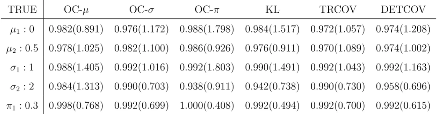
In Table 2, we report the performance of interval estimates, based on the percentage of intervals that covered their corresponding true parameters and the average interval width. From the table, we can see that all labeling methods had good coverage and exhibited higher-than-nominal rates of coverage in general. Based on Table 2, we can see that no single labeling method provided shorter intervals for all parameters. However, in general, OC-σ,T RCOV and DET COV provided shorter interval width than OC-µ, OC-σ, and KL for most of parameters.
−2 −1 0 1 2 −2 −1 0 1 2 OC σ 1 − σ 2 μ1−μ2 −2 −1 0 1 2 −2 −1 0 1 2 KL σ 1 − σ 2 μ1−μ2 −2 −1 0 1 2 −2 −1 0 1 2 TRCOV σ 1 − σ 2 μ1−μ2 −2 −1 0 1 2 −2 −1 0 1 2 DETCOV σ 1 − σ 2 μ1−μ2
Figure 1: Plots of σ1−σ2 vs. µ1−µ2 for the four labeling methods in Example 1. The black
0 0.5 1 −2 −1 0 1 2 OC σ 1 − σ 2 π1 0 0.5 1 −2 −1 0 1 2 KL σ 1 − σ 2 π1 0 0.5 1 −2 −1 0 1 2 TRCOV σ 1 − σ 2 π1 0 0.5 1 −2 −1 0 1 2 DETCOV σ 1 − σ 2 π1
Figure 2: Plots of σ1−σ2 vs. π1 for the four labeling methods in Example 1.
Table 1: Average (RMSE) of Point Estimates Over 500 Repetitions
TRUE OC-µ OC-σ OC-π KL TRCOV DETCOV
µ1 : 0 -0.010(0.152) 0.057(0.200) 0.204(0.282) 0.119(0.247) 0.038(0.199) 0.059(0.204) µ2 : 0.5 0.605(0.198) 0.538(0.202) 0.391(0.158) 0.476(0.195) 0.557(0.211) 0.536(0.201)
σ1 : 1 1.232(0.327) 1.089(0.177) 1.281(0.396) 1.180(0.322) 1.095(0.184) 1.110(0.204)
σ2 : 2 1.858(0.246) 2.001(0.139) 1.810(0.224) 1.910(0.181) 1.996(0.143) 1.981(0.156)
π1 : 0.3 0.413(0.140) 0.360(0.108) 0.281(0.057) 0.305(0.089) 0.362(0.109) 0.342(0.113)
Example 2 (Acidity Data): We consider the acidity data set (Crawford et al., 1992;
Crawford, 1994). The data are shown in Figure 3. The observations are the logarithms of an acidity index measured in a sample of 155 lakes in north-central Wisconsin. This data set has been analyzed as a mixture of Gaussian distributions by Crawford et al. (1992); Crawford (1994); Richardson and Green (1997). Based on the result of Richardson and Green (1997), the posterior for three components was largest. Hence, we fit this data set by a three-component normal mixture. We post processed the 20,000 Gibbs samples by the OC, KL, TRCOV, and DETCOV labeling methods. The runtime for KL, TRCOV, and DETCOV were 45, 2, and 6 seconds, respectively.
Table 2: Percent Coverage (average width) of Nominal 95% Interval Estimates Over 500 Repetitions
TRUE OC-µ OC-σ OC-π KL TRCOV DETCOV
µ1 : 0 0.982(0.891) 0.976(1.172) 0.988(1.798) 0.984(1.517) 0.972(1.057) 0.974(1.208) µ2 : 0.5 0.978(1.025) 0.982(1.100) 0.986(0.926) 0.976(0.911) 0.970(1.089) 0.974(1.002) σ1 : 1 0.988(1.405) 0.992(1.016) 0.992(1.803) 0.990(1.491) 0.992(1.043) 0.992(1.163) σ2 : 2 0.984(1.313) 0.990(0.703) 0.938(0.911) 0.942(0.738) 0.990(0.730) 0.958(0.696) π1 : 0.3 0.998(0.768) 0.992(0.699) 1.000(0.408) 0.992(0.494) 0.992(0.700) 0.992(0.615) 2.5 3 3.5 4 4.5 5 5.5 6 6.5 7 7.5 0 5 10 15 20 25 30 log(index) Histogram of acidity data
Figure 3: Histogram of acidity data. The number of bins used is 20.
It is difficult to use the similar graphic way in Example 1 to compare different labeling methods when the number of components is larger than two (Yao and Lindsay, 2009). Here, we mainly provided the trace plots and the marginal density plots to illustrate the success of DETCOV. Figure 4 and 5 are the trace plots and the estimated marginal posterior density plots, respectively, for the original samples and the labeled samples by DETCOV. (The OC, KL, and TRCOV methods had similar visual results to DETCOV for those plots.) From these figures, one can see that the DETCOV method successfully removed the label switching in the raw output of the Gibbs sampler.
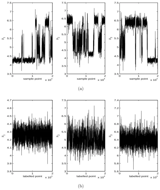
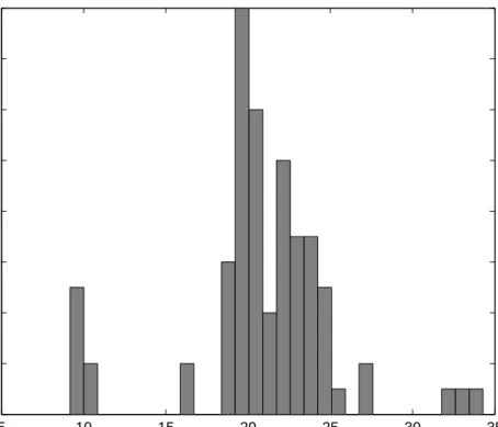
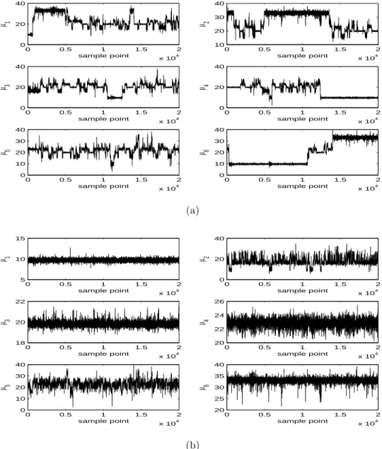
Example 3 (Galaxy Data): The galaxy data (Roeder, 1990) consists of the velocities (in thousands of kilometers per second) of 82 distant galaxies diverging from our own galaxy. They are sampled from six well-separated conic sections of the corona borealis. A histogram of the 82 data points is shown in Figure 6. This data set has been analyzed by many researchers including, for example, Crawford (1994); Chib (1995); Carlin and Chib (1995); Escobar and West (1995); Phillips and Smith (1996); Richardson and Green (1997). Stephens (2000) also used this data set to explain the label switching problem. We fit this data by six-component normal mixture. We post processed the 20,000 Gibbs samples by the OC, KL, TRCOV, and DETCOV labeling methods.
The runtime for KL, TRCOV, and DETCOV were 2487, 47, and 1161 seconds, respec-tively. Hence, the TRCOV method is much faster than KL and DETCOV.
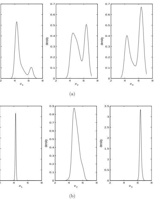
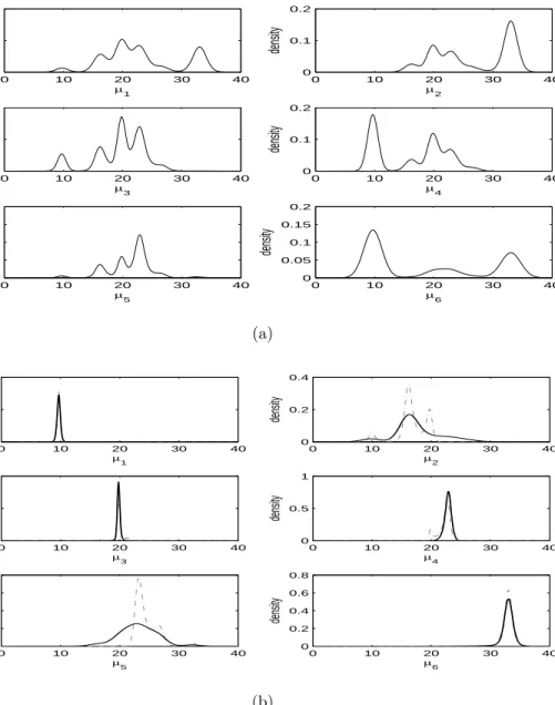
Figure 7 and 8 are the trace plots and the estimated marginal posterior density plots, respectively, for the original samples and the labeled samples by DETCOV. For the marginal density plot, for comparison, we also add the OC labels. In this example, for trace plots, there is no big visual difference for the four labeling methods. For marginal density plots, the TRCOV methods had similar visual results to OC and the KL methods had similar visual results to DETCOV. From Figure 7 and 8, one can see that the DETCOV method successfully removed the label switching in the raw output of the Gibbs sampler. Based on Figure 8, one can see that the DETCOV method removed the multimodality of the marginal posterior densities of the means in the raw output, however the OC method did not remove the label switching very well. Therefore, in this example, the DETCOV and KL methods worked a little better than the OC and TRCOV methods.
Based on the above simulation study and the real data set application, one can see that DETCOV usually works better than the OC, KL, and TRCOV methods. In addition, TRCOV works better than the OC and comparable to KL but TRCOV runs much faster than KL and DETCOV.
4
Summary
In this article, we proposed two new clustering related labeling methods. The first method TRCOV uses the idea of K-means clustering to label the samples. This method can be considered as an extension of the OC method. However, unlike the OC method, this method can simultaneously incorporate different component parameters together and can be easily extended to the high dimension case. In addition, as shown in Section 3, this labeling method is computationally much faster than the KL and DETCOV methods. The second method DETCOV is to label the samples by minimizing the volume of the labeled samples. This method is invariant to the linear transformation of the parameters. Based on the examples in Section 3, we can see that the DETCOV method successfully removed the label switching in the raw output. Our simulations also have shown that the TRCOV and DETCOV methods can produce good point and interval estimates.
In addition, our proposed methods TRCOV and DETCOV might also be able to solve label switching for frequentist mixtures since our methods only depend on the parameter samples. For frequentist mixtures, if one wants to use bootstrap method to estimate the variation of the parameter estimates, one needs to bootstrap the new data set and finds the corresponding parametric estimates for, say, N times. Let {θ1, . . . ,θN} be theN bootstrap
samples, which have meaningless labels. Similar to the Bayesian mixtures, one needs to solve the label switching problem for theN bootstrap samples before using them to estimate the variation. For bootstrap method, the data sets x = (x1, . . . , xn) are different for different θjs and thus the classification probabilities are not well defined, since they require to use
the same data set for all the parameter samples. Therefore, any labeling methods related to the classification probabilities, such as the KL algorithm, can not be applied. As far as we know, solving label switching for frequentist mixtures have not been well studied. This requires further research.
are not online algorithms. Users need to store all the samples before doing labeling. In addition, if the number of componentsmis too large or the dimension of the data is large, the DETCOV method might have numerical problems due to the calculation of C<t>−1 defined in
(2.3). If this problem occurs, one could use a ridge type estimator forC<t>−1 , say (C<t>+λI)−1
for some constant λ.
Based on the equivalence between the labeling and clustering if only one permutation of each sample is allowed in each of them! clusters, one can also apply other clustering methods or criteria to do labeling.
5
Acknowledgements
I am grateful to the editor, the associate editor, and the two referees for their insightful comments and suggestions, which greatly improved this article. In addition, I am indebted to my dissertation advisor, Bruce G. Lindsay, for his assistance and counsel in this research.
APPENDIX: PROOFS
Proof of Theorem 2.2: For simplicity, suppose that there are only two unknown component
parameters, such as component mean µ and component variance σ2, for each component.
Let θt= (ξTt1,ξ T
t2)T, where ξt1 is the m component means and ξt2 is m component variance.
Suppose M = N X t=1 (θωt t −θc)(θωt t−θc)T = A B B C ,
where A, B, and C are all m×m matrix. Let ˜ξt1 =a1+b1ξt1, ˜ξt2 =a2+b2ξt1 for all t and
˜
θc be the corresponding transformation of θc (See Theorem 2.3). Then
˜ M = N X t=1 (˜θωt t −θ˜c)(˜θ ωt t −θ˜c)T = b2 1A b1b2B b1b2B b22C .
Based on some matrix algebra, we have
det(M) = det A B B C = det(A) det(C−BA −1B). So det( ˜M) = det b21A b1b2B b1b2B b22C = det(b21A) det(b22C−b22BA−1B) =b2m1 b2m2 det(A) det(C−BA−1B) =b2m1 b2m2 det(M).
So for the linear transformation, the determinant of covariance criteria will not change, up
to a multiplication constant and thus the found labels will not change.
Proof of Theorem 2.3: Let
¯ θ= 1 N N X t=1 θωt t .
Note that det N X t=1 (θωt t −θc)(θωt t −θc)T ! = det N X t=1 (θωt t −θ¯)(θω t t −¯θ) T +N(¯θ−θ c)(¯θ−θc)T ! ≥det N X t=1 (θωt t −θ¯)(θω t t −θ¯) T ! , since θ¯−θc)(¯θ−θc)T
≥ 0. So the minimum of (2.2) over θc occurs at the sample mean
of {θ1, . . . ,θN}.
Proof of Theorem 2.4: Note that
C<t> =C−(θωt t −θc)(θωt t−θc)T =C1/2(I−utuTt)C 1/2,
where ut=C−1/2(θωt t −θc). By some calculation, we can verify
(I−utuTt) −1 = I+ 1 1−uT tut utuTt . So C<t>−1 =C−1/2 I + 1 1−uT tut utuTt C−1/2. Let vt=C −1/2 <t> (θω t t −θc)C −1/2 <t> . We have C=C<t>+ (θt−θc)(θt−θc)T =C 1/2 <t>(I+vtvtT)C 1/2 <t>. Note that (I+vtvtT) −1 = I− 1 1 +vT t vt vtvTt
So C−1 =C<t>−1/2 I − 1 1 +vT t vt vtvTt C<t>−1/2.
0 1 2 x 10⁴ 3.5 4 4.5 5 5.5 6 6.5 7 7.5 μ 1 sample point 0 1 2 x 10⁴ 3 3.5 4 4.5 5 5.5 6 6.5 7 7.5 μ 2 sample point 0 1 2 x 10⁴ 3.5 4 4.5 5 5.5 6 6.5 7 7.5 μ 3 sample point (a) 0 1 2 x 10⁴ 3.8 3.9 4 4.1 4.2 4.3 4.4 4.5 4.6 4.7 μ 1 labelled point 0 1 2 x 10⁴ 3 3.5 4 4.5 5 5.5 6 6.5 7 7.5 μ 2 labelled point 0 1 2 x 10⁴ 5.6 5.8 6 6.2 6.4 6.6 6.8 7 7.2 7.4 μ 3 labelled point (b)
Figure 4: Trace plots of the Gibbs samples of component means for acidity data: (a) original Gibbs samples; (b) labeled samples by DETCOV.
2 4 6 8 0 0.2 0.4 0.6 0.8 1 1.2 1.4 μ1 density 2 4 6 8 0 0.1 0.2 0.3 0.4 0.5 0.6 0.7 μ2 density 2 4 6 8 0 0.1 0.2 0.3 0.4 0.5 0.6 0.7 μ3 density (a) 2 4 6 8 0 1 2 3 4 5 6 7 μ1 density 2 4 6 8 0 0.1 0.2 0.3 0.4 0.5 0.6 0.7 0.8 0.9 μ2 density 2 4 6 8 0 0.5 1 1.5 2 2.5 3 3.5 μ3 density (b)
Figure 5: Plots of estimated marginal posterior densities of component means for acidity data based on: (a) original Gibbs samples; (b) labeled samples by DETCOV.
5 10 15 20 25 30 35 0 2 4 6 8 10 12 14 16
0 0.5 1 1.5 2 x 10⁴ 0 20 40 μ 1 sample point 0 0.5 1 1.5 2 x 10⁴ 10 20 30 40 μ 2 sample point 0 0.5 1 1.5 2 x 10⁴ 0 20 40 μ 3 sample point 0 0.5 1 1.5 2 x 10⁴ 0 20 40 μ 4 sample point 0 0.5 1 1.5 2 x 10⁴ 0 10 20 30 40 μ 5 sample point 0 0.5 1 1.5 2 x 10⁴ 0 10 20 30 40 μ 6 sample point (a) 0 0.5 1 1.5 2 x 10⁴ 5 10 15 μ 1 sample point 0 0.5 1 1.5 2 x 10⁴ 0 20 40 μ 2 sample point 0 0.5 1 1.5 2 x 10⁴ 18 20 22 μ 3 sample point 0 0.5 1 1.5 2 x 10⁴ 20 22 24 26 μ 4 sample point 0 0.5 1 1.5 2 x 10⁴ 0 10 20 30 40 μ 5 sample point 0 0.5 1 1.5 2 x 10⁴ 20 25 30 35 40 μ 6 sample point (b)
Figure 7: Trace plots of the Gibbs samples of component means for galaxy data: (a) original Gibbs samples; (b) labeled samples by DETCOV.
0 10 20 30 40 0 0.1 0.2 μ1 density 0 10 20 30 40 0 0.1 0.2 μ2 density 0 10 20 30 40 0 0.1 0.2 μ3 density 0 10 20 30 40 0 0.1 0.2 μ4 density 0 10 20 30 40 0 0.1 0.2 0.3 0.4 μ5 density 0 10 20 30 40 0 0.05 0.1 0.15 0.2 μ6 density (a) 0 10 20 30 40 0 1 2 μ1 density 0 10 20 30 40 0 0.2 0.4 μ2 density 0 10 20 30 40 0 1 2 μ3 density 0 10 20 30 40 0 0.5 1 μ4 density 0 10 20 30 40 0 0.1 0.2 0.3 0.4 μ5 density 0 10 20 30 40 0 0.2 0.4 0.6 0.8 μ6 density (b)
Figure 8: Plots of estimated marginal posterior densities of component means for galaxy data based on: (a) original Gibbs samples; (b) labeled samples by DETCOV (line) and labeled samples by OC (dash-dot).
References
Bo¨hning, D. (1999).Computer-Assisted Analysis of Mixtures and Applications, Boca Raton,
FL: Chapman and Hall/CRC.
Carlin, B. P. and Chib, S. (1995). Bayesian model choice via Markov chain Monte Carlo
methods. Journal of Royal Statistical Society, B57, 473-484.
Celeux, G. (1998), Bayesian inference for mixtures: The label switching problem. In
Comp-stat 98-Proc. in Computational Statistics(eds. R. Payne and P.J. Green), 227-232.
Phys-ica, Heidelberg.
Celeux, G., Hurn, M., and Robert, C. P. (2000). Computational and inferential difficulties
with mixture posterior distributions. Journal of the American Statistical Association, 95,
957-970.
Chib, S. (1995). Marginal likelihood from the Gibbs output. Journal of American Statistical
Association, 90, 1313-1321.
Chung, H., Loken, E., and Schafer, J. L. (2004). Difficulties in drawing inferences with
finite-mixture models: a simple example with a simple solution.The American Statistican,
58, 152-158.
Crawford, S. L., Degroot, M. H., Kadane, J. B., and Small, M. J. (1992). Modeling lake-chemistry distributions-approximate Bayesian methods for estimating a finite-mixture
model. Technometrics, 34, 441-453.
Crawford, S. L. (1994). An application of the Laplace method to finite mixture distributions.
Journal of the American Statistical Association, 89, 259-267.
study of perinatal mortality using a two-component mixture model. In Bayesian
Biostatis-tics (eds. D.A. Berry and D.K. Stangl) 601-616, Dekker, New York.
Diebolt, J. and Robert, C. P. (1994). Estimation of finite mixture distributions through
Bayesian sampling. Journal of Royal Statistical Society, B56, 363-375.
Escobar, M. D. and West, M. (1995). Bayesian density estimation and inference using
mix-tures. Journal of the American Statistical Association, 90, 577-588.
Fru¨hwirth-Schnatter, S. (2001). Markov chain Monte Carlo estimation of classical and
dy-namic switching and mixture models. Journal of the American Statistical Association, 96,
194-209.
−−(2006), Finite Mixture and Markov Switching Models, Springer, 2006.
Gallegos, M.T. and Ritter, G. (2005). A robust method for cluster analysis.Annals of
Statis-tics, 33, 347-380.
Geweke, J. (2007). Interpretation and inference in mixture models: Simple MCMC works.
Computational Statistics and Data Analysis, 51, 3529-3550.
Grun, B. and Leisch, F. (2009). Dealing with label switching in mixture models under genuine
multimodality. Journal of Multivariate Analysis, 100, 851-861.
Hurn, M., Justel, A., and Robert, C. P. (2003). Estimating mixtures of regressions. Journal
of Computational and Graphical Statistics, 12, 55-79.
Jasra, A, Holmes, C. C., and Stephens D. A. (2005). Markov chain Monte Carlo methods
and the label switching problem in Bayesian mixture modeling. Statistical Science, 20,
Lindsay, B. G., (1995), Mixture Models: Theory, Geometry, and Applications. NSF-CBMS Regional Conference Series in Probability and Statistics v 5, Hayward, CA: Institure of Mathematical Statistics.
Marin, J.-M., Mengersen, K. L. and Robert, C. P. (2005). Bayesian modelling and inference
on mixtures of distributions.Handbook of Statistics25 (eds. D. Dey and C.R. Rao),
North-Holland, Amsterdam.
McLachlan, G. J. and Peel, D. (2000). Finite Mixture Models. New York: Wiley.
Phillips, D. B. and Smith, A. F. M. (1996). Bayesian model comparison via jump diffusion.
Makov Chain Monte Carlo in Practice, ch. 13, 215-239, London: Chapman and Hall. Richardson, S. and Green, P. J. (1997). On Bayesian analysis of mixtures with an unknown
number of components (with discussion). Journal of Royal Statistical Society, B59,
731-792.
Roeder, K. (1990). Density estimation with confidence sets exemplified by superclusters and
voids in the galaxies. Journal of American Statistical Association, 85, 617-624.
Rousseeuw, P. J. (1984). Least meadian of squares regression. Journal of the American
Statistical Association, 79, 871-880.
Stephens, M. (2000). Dealing with label switching in mixture models. Journal of Royal
Sta-tistical Society, B62, 795-809.
Walker, A. M. (1969). On the asymptotic behaviour of posterior distributions.Journal of the
Royal Statistical Society, B31, 80-88.
Yao, W. and Lindsay, B. G. (2009). Bayesian Mixture Labeling by Highest Posterior Density.