Lancaster University Management School
Working Paper
2005/005
Demand uncertainty and lot sizing in manufacturing
systems:
The effects of forecasting errors and mis-specification
Robert Fildes and Brian Kingsman
The Department of Management Science Lancaster University Management School
Lancaster LA1 4YX UK
© Robert Fildes and Brian Kingsman
All rights reserved. Short sections of text, not to exceed two paragraphs, may be quoted without explicit permission,
provided that full acknowledgement is given.
The LUMS Working Papers series can be accessed at http://www.lums.lancs.ac.uk/publications/
MS 01/97 (revised)
DEMAND UNCERTAINTY and LOT SIZING IN MANUFACTURING
SYSTEMS:
The effects of forecasting errors and mis-specification
Robert Fildes and Brian Kingsman Department of Management Science
Lancaster University Lancaster LA1 4YX Tel: 01524 - 593879 Fax: 01524 - 844885
Contact E-mail:
Correspondence to R. Fildes Revised: 21st December, 2004
DEMAND UNCERTAINTY and LOT SIZING IN MANUFACTURING
SYSTEMS:
The effects of forecasting and mis-specification
Robert Fildes and Brian Kingsman
This paper proposes a methodology for examining the effect of demand uncertainty and forecast error on lot sizing methods, unit costs and customer service levels in MRP type
manufacturing systems. A number of cost structures were considered which depend on the expected time between orders. A simple two-level MRP system where the product is manufactured for stock was then simulated. Stochastic demand for the final product was
generated by two commonly occurring processes and with different variances. Various lot sizing rules were then used to determine the amount of product made and the amount of materials bought in.
The results confirm earlier research that the behaviour of lot sizing rules is quite different when there is uncertainty in demand compared to the situation of perfect foresight of demand. The best lot sizing rules for the deterministic situation are the worst whenever there is
uncertainty in demand. In addition the choice of lot sizing rule between ‘good’ rules such as the EOQ turns out to be relatively less important in reducing unit cost compared to improving forecasting accuracy whatever the cost structure. The effect of demand uncertainty on unit cost for a given service level increases exponentially as the uncertainty in the demand data increases. The paper also shows how the value of improved forecasting can be analysed by examining the effects of different sizes of forecast error in addition to demand uncertainty. In those
manufacturing problems with high forecast error variance, improved forecast accuracy should lead to substantial percentage improvements in unit costs.
1. INTRODUCTION
MRP systems are in widespread use for co-ordinated production and operations planning in
manufacturing systems. These typically assume a deterministic environment with the emphasis on co-ordinating production at all levels and the purchasing of components and materials so as to meet the
planned Master Production Schedule (MPS). The MPS provides the linkage between the demands of the outside customers and the detailed planning and scheduling of internal production supply facilities.
The MPS, once determined, is passed onto the material requirements planning system. Uncertainty can affect the performance of the MRP system in a variety of ways. Random variations can occur in internal manufacturing lead times, in purchasing lead times or stochastic yield variations at production
stages. Since these latter activities mainly fall within the span of control of the company management,
they can be managed in order to reduce significantly the amount and impact of uncertainty. External demand from customers is however normally outside the company’s control, except for gross
influences like promotions, and is stochastically varying over time in most practical situations. Thus the MPS has to be developed on the basis of forecasts of demand.
The scheduled production will either be insufficient to meet the realised actual demand, thus
producing shortages, or exceed the realised demand resulting in unanticipated stocks. As several
authors have pointed out, for example Vargas and Dear (1991), the effect of demand uncertainty on simple deterministic lot-sizing techniques, and their corresponding effectiveness, such as are
commonly used in MRP applications, is an important problem. While all researchers seem to agree
with the conclusions of De Bodt and Van Wassenhove (1983a) and others that demand uncertainty dramatically increases lot-sizing costs, the simple questions, of how those costs increase with
forecasting error and the relationship to demand uncertainty, how different lot sizing rules perform and
whether the form of demand pattern and the forecasting model used are important, remain unresolved. The contribution made in this paper is thus to integrate two distinct research areas, manufacturing systems and forecasting.
In order to investigate this problem researchers must make a number of choices, (i) on the form of the MRP system, including the number of levels and the interdependence within the production
process, production/ delivery lead times, and back-ordering rules, (ii) the lot sizing rules to be considered and their application at differing levels of the MRP system, and, (iii) the costing of the
important issues for research in this area, as explored further in the next section, are the form of the demand and forecast functions. These issues include the levels of forecast error to be included in the
experimental design, and how possible bias is to be treated. It is questionable whether previous published research has treated these issues correctly.
Researchers have tackled the problem of uncertainty in MRP systems in two distinct ways: firstly, through case studies with changes in forecast errors arising from the use of different forecasting
methods (Gardner, 1990, Lee et al., 1993, Enns, 2002 ) and, secondly, through developing a simulation of the whole MRP system, including the demand distribution and forecast errors. This paper adopts the second approach with the aim of developing a satisfactory methodology for quantifying the effects
of forecast error in manufacturing systems.
The production system simulated here is composed of two stages, a raw material (or a
component) having a purchasing and delivery lead time and a manufacturing process (or assembly) to
make the final product from the material ( or component), requiring one or more periods to be completed. The major areas of interest in the simulation experiment are the costs of producing the final product and the customer service level achieved, together with the effect of demand forecast
errors. The research presented follows most earlier work in assuming the only stochastic variation is
in the demand for the final products. It is assumed that internal manufacturing lead times and purchasing lead times are fixed and also that internal yields are always 100%. The components are pushed up to the final level as scheduled. They are not delayed because the demand for the final
product has changed. All variation is absorbed into the stock of finished items. The methodology we describe here extends straightforwardly to more complex production systems with manufacturing
uncertainty, interdependent demand and capacity constraints. This paper is in six further sections. We
next consider demand uncertainty and appropriate ways of specifying the forecast error. Section three describes the simulated manufacturing system including costs and lot sizing rules while section four describes the simulation experiment. The substantive results of the simulation are presented in section
5 for differing levels of demand uncertainty. Section 6 considers the effects of different forms of forecast error and forecasting model misspecification (in addition to the demand uncertainty). The
paper concludes with a discussion of the results, both substantive and methodological.
The results provide conclusive evidence that the forms of the demand and forecast functions
the impact is both economically significant for typical values of the demand parameters and increases substantially as forecast error increases. Estimates of the effects of forecast error are included -
improvements in forecasting accuracy are worth achieving only if the absolute level of accuracy improves markedly. In addition, the form of the demand function and any specification error is shown
to be significant. Equally important, the paper demonstrates an effective methodology for investigating the effects of forecast error on manufacturing systems.
2. DEMAND UNCERTAINTY AND FORECAST ERRORS IN MANUFACTURING SYSTEMS
Many studies have evaluated the performance of simple deterministic lot-sizing rules in
manufacturing systems and the effects of uncertainty on the various rules have also generated considerable interest, with Wemmerlov (1989) offering an early summary. The problems with the
earlier research include a limited range of lot sizing rules, (Vargas and Dear, 1991), and a lack of clarity in distinguishing between demand uncertainty and forecast error, (De Bodt and Van Wassenhove, 1983a, Lee and Adam, 1986). The lot sizing rules examined by these researchers
included those commonly adopted in organisations - more complex stochastic rules that take into
account the demand distribution were excluded. While much of the research analysed a simple production system (e.g. De Bodt and Wassenhove, 1983b, Lee and Adam, 1986, Ritzman and King, 1993, Chen et al, 2000a) a few researchers have considered MRP systems closer to the complexity
observed in practice e.g. Vargas and Dear, 1991, Enns, 2002. The problem with the more complex studies is that the quantitative results are likely to be specific to the distinctive features of the chosen
production system. More particularly, unless due care is taken in choosing the criteria by which
performance is evaluated, the results will follow automatically from the choice of cost parameters. For example, if service level is not taken into account (Lee and Adams, 1986) then lot-sizing rules which lead to low inventories and correspondingly low service levels will automatically be preferred.
While not discounting the need to examine complex systems we will follow the approach adopted by Wemmerlov and Whybark (1984) and Wemmerlov (1989). These studies examined a
single level, single product production system in a rolling horizon environment. The conclusion of Wemmerlov’s research (1989) gave further support to De Bodt and Van Wassenhove (1983a) - that an
that results from the latter case will not apply in most practical situations. He also found no significant difference in performance between the six best lot-sizing rules when demand was uncertain,
concluding that this diminished the value of lot-sizing research. (However some other common rules performed poorly; nor was economic impact considered).
The inadequate incorporation of service level has led to further confusion in past research: failing to distinguish between the (unknown) bias in the forecast, and a buffering strategy of forecast
inflation that aims to moderate the effects of forecast errors by increasing the forecast (Lee and Adam, 1986). Such a buffering strategy has long been criticised as inadequate in simple production systems when compared to the alternative of using safety stocks, e.g. Vargas and Dear (1991).
In an attempt to overcome the major problem of service level associated with most of the
previous work Wemmerlov (1989) partially controlled for service level by using a buffer to ensure that the service level was 100%. In the research described here we go further by considering a two level
production system including service level as a continuous variable. This permits us to evaluate the effects of realistic improvements in forecasting accuracy on differing levels of service and unit costs.
2.1 Demand Models Used In MRP Research
Earlier authors when examining the effects of uncertainly on MRP systems have considered only limited models of the demand generation process and forecast function. De Bodt and Van
Wassenhove (1983a, 1983b) compared various lot sizing rules when demand was generated by dt =µd
+ εt where εt is N(0,σ2) and µd is constant. The demand forecasts were derived using exponential
smoothing. They concluded that with any level of demand uncertainty greater than zero total costs were increased about 10%; the impact was highest when ordering costs were low compared to
inventory costs (and the time between orders was therefore short). Also, the choice of lot-sizing rule was unimportant with the exception of Lot-for-Lot which performed uniformly poorly. Mean demand
was set at 200 and σ varied from 0 to 50 giving corresponding coefficients of variation (CV) of 0 to
0.25. The MRP system was such that current demand was known and could be immediately supplied. There were therefore no stockouts. This key assumption limits the usefulness of their work. They also
fail to match their generation process for demand (random about a constant level) to their forecasting method (exponential smoothing which is non-stationary). This is a common mistake (see for example,
mis-specification error which makes interpretation of their results difficult.
Lee and Adam (1986) and Lee, Adam and Ebert (1987) examined more complex MRP
systems. Demand was generated by dt = µd, a constant while the forecasts were seen as randomly
distributed around µd, as N(δ, σ2) where δ is the bias in the forecast. Lot-for-Lot again performed
poorly. A wide range for the coefficient of variation was considered. Despite the wide range, the error
standard deviation had little effect on performance while the bias was evaluated as much more
important. However the more extreme values within Lee and Adam’s simulation and the specification
of the demand generating function can be dismissed as unrealistic, both in form and for their choice of error distribution parameters, see Fildes and Beard (1992) and Fildes et al (2004). The conclusion they
drew that the bias was the more important factor again arises from the cost parameters considered. More recently, research has focussed on bullwhip effects and supply chain coordination, (see for example, Chen et al, 2000a, 2000b, Xu et al, 2001 Zhao et al, 2001). While more care has been taking
in specifying both the DGP and the forecasting model one of their fundamental and unanalysed
assumptions is that the forecasting model used by the manufacturer is mis-specified.
2.2 Independent Demand and Corresponding Forecasting Methods
Although a plethora of different forecasting methods have been proposed as suitable for forecasting independent demand, recent large scale empirical studies have concluded that a limited range of simple methods perform as well as their more complex alternatives, (Fildes and Makridakis, 1995, Makridakis et al, 2000, Fildes et al, 2004). Particularly for monthly or weekly data on item demand, simple autoregressive statistical models should adequately characterise most of the situations encountered in practice. Two simplifications from the typical series observed in practice have been made here: extreme (or outlying) observations have been neglected and the data are assumed to be non-seasonal. The effects of these assumptions require further research. We therefore propose to analyse the following demand model, where Dt is the demand in period t and et is random white noise:
1
1 −
− + −
+
= t t t
t D e e
D δ ρ θ
This model, which is a realistic generalisation of earlier work, includes a wide range of data
types that are commonly observed in practice as the forecasting literature has established, see for
example, Fildes et al (2004). For ϑ=ρ=0 the model is just the ‘constant mean demand model’ (contrast
the Lee and Adam’s formulation described earlier) while for ρ=1 and ϑ <1 the model is the ARIMA
the model is a stationary AR(1) process. The above model is the basis of the most common forecasting methods used in production systems.
The optimal one-step ahead forecast of demand for period t, made in period t-1 after that demand is known, for the above data generation process is given by:
1 1
-+ =
1,t Dt− et−
t-F
opt δ ρ θ
The error term, et-1, is the forecast error observed in the previous period, the difference between the
realised demand and the forecast and, at time t, is non-stochastic. In general, of course, such an
optimal forecast would be unavailable to the scheduler, not least because the parameters would have to
be estimated from the data. In this study we assume the parameters are known exactly; the only difference between the optimal forecast and the data generation process arises because of the random
error, et.
Two particular demand models are considered in the research as follows:
(i) δ= 1000, ρ = 0, θ = 0: the constant demand model, with mean level, 1000, hence
e + 1000 = D and 1000 =
F t t
t 1, -t
opt
(ii) δ = 100, ρ = 0.9, θ= 0: an almost non-stationary process, with mean level 1000, hence
t -1,t t -1 t t -1 t
opt F = 100 + 0.9D and D = 100 + 0.9D + e
The distribution assumed for et includes a range of values for the noise variance but the mean
is assumed to be zero. The reason for this choice is that a constant bias model (such as that used by Lee and Adam) would be forecastable over time. The noise distribution is assumed normal (although
demand and the forecasts of demand are constrained to be positive). Additional research is needed to examine the effects of non-normal errors and outlying observations which are often observed in
demand data. The general form for the forecast error variance for an AR(1) model for k steps ahead is :
var ( ) ( )
( )
e kt = − k − 1 1 2 2 2 ρ ρ σ
For the constant demand model, with θ = 0, the forecast error variance is constant for all steps ahead.
steps ahead and 2.201 for 12 steps ahead.
The complete specification of this data generation process depends on the values chosen for the
noise variance. The values used in the experiment represent a plausible range of values for fast
moving items according to surveys of forecasting accuracy reported in the literature (Fildes and Beard,
1992; Fildes et al, 2004). For one-step ahead (3 months ahead or less) forecasts, the average mean absolute percentage error (MAPE) was found to be 16%. For a normal distribution this roughly
translates into a coefficient of variation of 0.20. In the simulation experiment we will therefore use values of the coefficient of variation ranging from 0 to 0.4. For et assumed Normal the range of values of the noise standard deviation included in the simulation experiment are therefore: 0, 50, 100, 200,
400 (around a mean of 1000).
3. THE PRODUCTION AND LOT SIZING ENVIRONMENT
3.1 Planning Horizon and Action Horizon
In uncertain environments, MRP is usually developed using a rolling schedule. When using a rolling schedule, the production schedule is replanned at regular intervals. Decisions are made taking
into account the forecast demands over some future fixed planning horizon. In each successive period, lot-sizing decisions are made to minimise costs over the planning horizon ahead from that period.
Orders for raw material then are placed and production occurs. An ordering decision by the
manufacturer now leads to the scheduled arrival of that order some lead time into the future. Here it is
assumed that once orders have been placed, they cannot be cancelled or altered in any way. Thus a portion of the production schedule determined for the planning horizon is frozen each planning cycle.
This will include all those periods with the scheduled arrival of an outstanding order placed in previous periods. This frozen portion will be at least the maximum lead time, L, to produce the item through all
of the possible stages of purchasing and manufacturing. It may also include a further action horizon, a length of time, of say A periods, over which any recommended orders are made firm orders, which
cannot then be changed in later periods. Given the assumptions of constant processing and lead times, only the total length of the frozen period matters, not how the frozen period is decomposed into the
maximum manufacturing lead time and the action horizon.
number of periods over which demands can be batched into different lot sizes. The longer it is the greater the possibility of reducing costs by allowing bigger orders where advantageous. The total
planning horizon is the frozen plus free periods. The simulation model allows different values for both the frozen and free horizons to be examined. The experiments covered values of 2, 5 and 7 periods for
the frozen period and 12, 24 and 36 for the free horizon.
3.2 Costs
The costs included in this experiment consist of the cost of placing orders and the cost of holding stock. There are two major measures of performance, (i) the average ordering and
stockholding costs per unit of demand and (ii) the service level achieved, defined as the proportion of
demand satisfied immediately either from the opening stock or the current period’s output.
Since most of the deterministic lot-sizing rules aggregate the net requirements over future time
periods to give the lot sizes, the expected time between successive orders is an appropriate method of ranking alternative sets of cost parameters, the ordering cost and (end of period) stockholding cost. This was determined from the order cycle given for the classical Economic Order Quantity (EOQ),
based on the average demand per period implied by the demand generation processes used. It is often
known as the Time Between Orders measure, TBO. The stockholding cost was set at 1 and the expected average period demand at 1000. Ordering cost values were chosen to give TBO values, measured in periods, in the middle of the ranges 1 - 2, 2 - 3, 3 - 4 and 4 – 5. These values imply the
order would be expected to cover 1, 2, 3, 4 and 5 periods’ demands respectively. The corresponding values for the ordering cost will then be1750, 3500, 7000, 11500. (A TBO of 1 was considered but has
quite different performance characteristics with EOQ incurring extra stockholding costs – this has
been omitted from the analysis.)
3.3 Service Level and Safety Stocks
A service level performance measure has been used rather than including stockout costs as part of the total cost, since the latter are almost impossible to estimate in any meaningful way in practice.
We adopted the approach of letting the service level, here defined as the fraction of total demand satisfied immediately from stock and current output, be a factor in the experiments. This allowed us to
forecast error conditions, different lot sizing rules result in different performance costs and different service levels. In order to render the results comparable, the models were run with different levels of
target end of period stocks. If this target level is a positive quantity then this is equivalent to holding safety stock. Lower service levels are only possible by deliberately forcing the system on average to
have stockouts. This can be achieved by allowing backorders or lost sales up to some pre-set level, i.e. by making the safety margin negative.
3.4 Lot Sizing Model for Backorders and Lost Sales Case.
As discussed above, the existence of an action horizon, A, means that at any time, t,
recommended orders to be placed within the next A periods are made up of firm orders which cannot be changed at a later time. Thus at time t, orders already placed for periods t+1 to t+A-1 are
outstanding orders that were placed at an earlier time and cannot be altered in any way. These orders will arrive a lead time L after they were placed, in periods t+1+L to t+A-1+L. Let us denote the frozen interval as discussed above, the sum of the action horizon and the lead time in periods, as F = A-1+L. Thus, lot sizing decisions taken at time t cannot affect the backorders or lost sales arising over the frozen part of the schedule, periods t+1 to t+F but start only for orders that will arrive in periods t+F+1 onwards. The problem is therefore to find the orders from this period t+F+1 onwards that minimise the costs of meeting the forecast demand over the next F+P periods where P is the planning horizon. Let Ft,t+k be the forecast of demand (plus any buffer) for period t+k made at the end of period t, after the demand for period t is known, for k = 1 to F+P. There are outstanding orders from earlier periods, OOt+k, scheduled to arrive for period t+k for k = 1 to F. Let It,t be the known stock at the end of period t. It,t+k is defined as the stock projected for the end of period t+k on the basis of the forecast period demands, outstanding orders and the ordering decisions made in period t.
Different service levels are generated by specifying the target stock levels to be achieved at the
end of every period including buffers. Unlike the standard lot sizing procedure for deterministic demands, the aim here is to ensure that the projected start of period stock plus the order scheduled to
arrive at the start of that period less the forecast demand is at least some specified stock level, SS. If SS is positive then it is a safety stock to guard against demand variations. If SS is negative, then it is
the maximum level of backorders that can be planned to be carried from one period to the next or the maximum shortfall in meeting the predicted demand for a period in the lost sales case. So in lot size
planning in period t, new orders should be scheduled to arrive in period t+k, O*t,t+k, to ensure that
treating the forecasts as realised demands. The lot sizing problem at the end of period t can thus be
expressed as to determine the orders scheduled for arrival in period k, O*t,t+k, that minimise the total costs of ordering and stockholding over periods t+F+1 to t+F+P whilst satisfying the above constraint
for all periods.
(
)
[
]
∑
+PF 1 + F = k k + t t, h k + t t,
o
C
I
C
+ Max 0,
Minimise
δ
(2)where Co is the ordering cost and Ch the inventory holding charge per unit, and δt,t+k is an indicator
representing whether an order is placed in period t+k to arrive in period t+k+L.
For the backorders case, it can be shown, see Fildes and Kingsman (1997), that independently of whether SS is positive or negative, the introduction of the target end of period stock levels, SS,
requires the determination of the best lot sizes to meet the net requirements (NRt,k ) for each period
over the P period planning horizon from k= t+F+1 to t+F+P, which are given for j = 1 to P by
t t F j
NR Min Ft t j Max Ft t k
k
F j
SS It t F
, + + = , + F + , , , +
= F + + + - , + 0 1 ∑ ⎧ ⎨ ⎩ ⎫ ⎬ ⎭ ⎧ ⎨ ⎩ ⎫ ⎬ ⎭ (3)
where It,t+F is given by continuously applying the stock transition equation (2) above with O*t,t+k = 0 over the frozen part of the schedule, the periods k = 1 to k = F. It can be seen that any backorders occurring over the frozen part of the schedule are cumulated until period t+F+1 and then added to the forecast demand for period t+F+1. Adding in NRt,t+k = 0 for k = 1 to F, this provides the forecast net requirements that must be satisfied over the planning horizon F + P for lot sizing planning at each time period t, using various lot sizing algorithms. The problem remains deterministic for lot size planning at the start of each period even when planned safety stocks or planned backorders are allowed. Since it has been expressed as determining the lot sizes to minimise the ordering and stockholding costs of meeting a given set of demands, it satisfies the conditions for which the standard lot sizing heuristics were devised.
3.5 Lot sizing rules
Six alternative lot-sizing methods were evaluated in the simulation, as given below. Fuller
cases, the currently uncovered net requirements over the free part of the planning horizon, taking account of any backorders that have accumulated, are firstly determined to give the demands to be
satisfied. The average period demand is the average of the uncovered net requirements divided by the total number of periods in the free part of the planning horizon. However, if the net requirement in the
first free period (or first few free periods) is zero then this is ignored in the averaging. In this
particular case, no order will be placed and the simulation moves on to the following period updating
the system with the actual period demand.
EOQ (Economic Order Quantity): The lot size is set equal to the standard Wilson Economic Order Quantity calculated on the basis of the average period demand, as above. If the EOQ is insufficient to
meet the first period’s net requirement, the lot size is made the smallest multiple of the EOQ that achieves this.
POQ (Period Order Quantity): This converts the EOQ lot size to the nearest integer number of periods demands, (again based on the average period demand over the free part of the planning horizon as above).
LUC (Least Unit Cost): The lot size is increased to cover succeeding periods until the item unit cost is at a minimum. The item unit cost is the ordering cost plus the stockholding costs for the lot divided by the lot size. If there is a tie, then the smaller number of periods is taken.
LTC (Least Total Cost or Part Period Balancing): This is based on the concept that the least total cost occurs where the ordering and stockholding costs are most equal. The lot size is increased to cover succeeding periods until the stockholding cost is closest to the ordering cost. Again, if there is a
tie, the smaller number of periods is taken.
Silver Meal Heuristic: The objective is to minimise the costs per period, so the total costs as in the LUC method are divided by the number of periods. If a period within the total covered by the lot has zero net requirement then it counts as a period for the division.
Wagner Whitin algorithm: This procedure gives the optimal solution for minimising the costs of meeting a given set of deterministic requirements over a given planning horizon.
methods are excluded from the analysis due to their consistently poor performance.
4. THE SIMULATION EXPERIMENT
Within the production system described in the previous section a number of arbitrary decisions
have been made that could affect the results we report. Demand has been generated over 20,000 periods but the variability of demand itself suggests it is wise to repeat the simulation experiment in
order to establish the effect on demand, service level and the various costs. Five replications were carried out and detailed examination analysis of these runs showed that there was very little difference between the outcomes of each of the replications. The safety stock was set as a buffering factor times
the forecast error deviation. The service level recorded was the average value over the 5 replications
for that buffering factor, and similarly for the unitcosts. The buffering values were chosen so as to cover service levels in the range 90% to 99.5%.
The random numbers used were generated using the Turbo Pascal function ‘random’ based on fixed seeds so that each experimental run used common random numbers to reduce variance when evaluating those factors determining unit cost (Law and Kelton, 1991). The normal distribution
generator was that proposed by Box-Muller (1958).
In addition the effects of the following parameters on the results have been examined:
(1) frozen interval - The experiment was run with three different frozen periods, 2 (the minimum possible given the two period nature of the production process), 5 and 7. The results reported in
this paper are for a frozen period of 5. Unsurprisingly the shorter the frozen interval, the lower the unit cost curve. The ranking of the LSRs remained essentially unchanged (average
correlation=.97). The change in the relative performance1 (when comparing results across frozen
intervals) is small, averaging around 1%.
Because the frozen interval determines the first period in which the schedule can be changed it also affects the actual error standard deviation under which the plans are set. The error standard
deviation for the first period in which the schedule can be changed, denoted by σ(F+1) where F is
error standard deviation; for the constant demand process the error deviation remains constant whatever the lead time.)
(2) planning horizon - the simulations were run with three different free planning horizons, 12 , 24 and 36 periods, for some options. Note that the full planning horizon is the relevant frozen interval
plus this free horizon. The results were virtually identical with an average correlation of .99 approximately. This was as expected because even the smaller free planning horizon is more than
twice the maximum TBO of between 4 and 5 periods. All the experiments reported are for a free planning horizon of 24 periods except where noted for the Wagner-Whitin algorithm.
(3) simulation run length and warm-up period - the experiment starts with zero stocks and zero demand over the frozen interval. The actual simulation period was for 20,000 periods, having first
‘run-in’ the simulation for a warm-up period of 72 periods. The warm-up period outcomes are not included in the analysis of the results
(4) validation – the programme was broken into a number of test sub-programs covering the lot sizing rules, the demand generation and the forecast generation processes and the rolling schedule
calculations. Each were verified against manual calculations.
5. THE EFFECTS OF DEMAND UNCERTAINTY WITH OPTIMAL FORECASTING The results of the various simulations are presented in terms of two key measures of performance as discussed earlier. The Total Cost(i,j) is the sum of the ordering costs and holding costs
incurred for the ith combination of experimental factors and the jth simulation replication. The mean unit cost for the ith combination of experimental factors is the average over the J replications, i.e.,
nd(i,j) Total Dema (i,j) Total Cost J i,j) Unit Cost( J i) Unit Cost( Mean j J j
∑
∑
= = = 1 1 1The total satisfied demand each period is that met immediately from stock or the current period’s output, so the mean service level for the ith combination of experimental factors is
∑
∑
==
j
j Total Demand(i,j)
d(i,j) sfiedDeman Total Sati J vel(i,j) Service Le J vel(i) Service Le
Mean 1 1
Experiments were performed on two demand processes. The first is the Constant Demand Data
Generation Process, where the period demands are essentially random variates from a normal distribution with a mean of 1000 and standard deviations ranging from 50 to 400. The second is a
more typical demand pattern in manufacturing, which is when there is a strong autoregressive pattern in the data. The case examined is Autoregressive parameter = 0.9. The overall variation in demand is
larger than for the constant mean demand case and there are apparent cycles in the data.
Figure 1a presents some examples of the trade off curves obtained for the various lot sizing
rules with a Constant demand DGP which show the mean unit cost(i) graphed against the mean service level(i)for each of the buffer values used in the experiments when there is perfect foreknowledge of
the future demands. This is the deterministic demand case for which the lot-sizing rules were originally designed. The results shown are for a TBO value of 5 and for two values for the error
standard deviation, 100 and 400. (It should be remembered that a TBO = 5 means that the average time
between orders is 4 periods, which is given by an ordering cost of 7000 relative to a period holding cost of 1). An immediate tentative finding from Figure 1 is that there is little difference between the
unit costs values of the rules for the lower error standard deviation, apart from the EOQ which costs significantly more, except for the lower service levels. The relative ordering of the unit costs of the lot
sizing rules remains the same over the whole range of service levels shown. The differences between the rules become larger as the error standard deviation increases. The ordering of the rules in terms of
unit costs, lowest cost first, is WW, SM, LTC, LUC, POQ and EOQ2. This is not new, it is typically
what has been found in previous studies . However, these results give a base level for comparison of the effects of demand uncertainty on the performance of the rules. The WW rule, of course, gives the
optimal solution over the planning horizon at each period in turn, allowing for the previous decisions. The SM rule is always second best and not far from the optimal WW. The EOQ performs worst
because its order size is not constrained to be the demands over a number of integer periods, leading to
carry-over stocks in every period.
2
[image:17.595.80.550.467.800.2]The optimality of Wagner-Whitin is not assured for a finite forecast horizon. Tests have shown for WW to be optimum for planning horizons greater than 90.
Figure 1: Unit Cost vs Service Level
Various Lot Sizing Rules: Time Between Orders 4 Periods
Figure 1a Perfect Information
[image:17.595.324.550.473.655.2]Demand Uncertainty=100
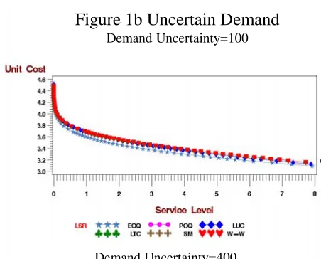
Figure 1b Uncertain Demand
Demand Uncertainty=100
Figure 1b shows the trade off curves obtained for the various lot sizing rules for the same case as in Figure 1a but now based on forecasts of the future demands each period. The ordering decisions are
based on the forecast of demands over the planning horizon at each period in turn, not the actual demands as for Figure 1a. Note that in this case, the unit costs become asymptotic with the vertical
axis as the service level tends to 100%. An immediate finding from Figure 1b is that there is again a consistent difference between the different lot-sizing rules over the whole range of service levels
shown, but that the differences are much smaller than those of Figure 1a, the deterministic demand situation with perfect foresight. The relative ordering of the unit costs of the lot sizing rules is the same for both levels of demand uncertainty but the differences becomes smaller as the noise standard
deviation increases. The other tentative finding is that ordering of the rules in terms of unit costs is the
reverse of what was found for the perfect foresight case. The EOQ is always the best, whilst the WW ‘optimal’ algorithm is almost always the worse. However, there is not a lot of difference between the
rules other than for the EOQ.
Graphs such as Figure 1 are an illuminating way of presenting complex results, but,
unfortunately, the service levels resulting for each lot sizing rule and level of demand uncertainty for
the same buffering factor (and hence safety stock) differ. Although one can draw general conclusions
from such figures, they do not allow the direct derivation of a quantitative summary of the relative performance for all costs structures and the different levels of the error variance for a particular Data Generating Processes. The solution to this difficulty was to model the trade off curves quantitatively
to give the relationship between the unit cost and the service level. They were modelled individually for each lot sizing rule, error deviation, data generation process and cost structure (TBO) by
loge(Unit Costi) = µ+β1(Service Leveli%)+β2( Service Leveli%)2
+ β3(Service level) .5
+β4(Service level) 3
.+lg(Service level)+ εi.
where i is the experimental setting. Various simpler alternative specifications were considered such as
a log-log function of mean service level but this flexible form was preferred. The curves were
estimated for the service level less greater than 90%. The maximum percentage error in predicted unit
cost is less than .1% with R2=1 in all cases. Different plausible functional led to the same rankings of the various LSRs.
relative performances. Two target service levels were selected, 99% and 96%, representing high and a more modest but acceptable level of service achievement. The detailed values by all TBOs from 2 to 5
and for all four error deviations are available from the author for both the Constant Demand and Autoregressive Demand DGPs.
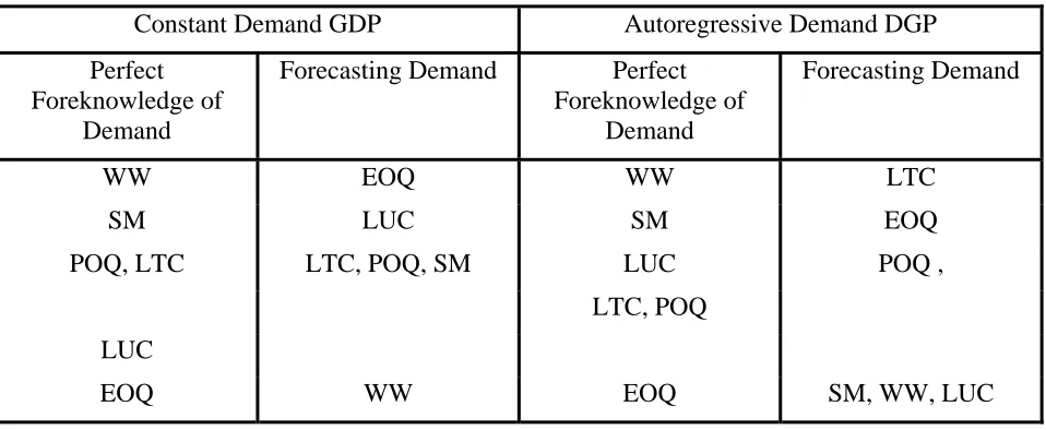
An analysis of ranking the lot-sizing rules performance by unit cost for each of the TBO and error deviation combinations confirmed the earlier result on their relative ordering, see Table 1. The
[image:19.595.53.532.334.531.2]ordering is as expected when there is perfect foreknowledge of demand for both demand DGPs. The optimal WW rule is first followed quite closely by SM. The EOQ is always worst
Table 1 – Ranking the Rules by Unit Cost
(measured by ranking each method for each TBO and level of noise uncertainty and summing the ranks)
Constant Demand GDP Autoregressive Demand DGP Perfect
Foreknowledge of Demand
Forecasting Demand Perfect Foreknowledge of
Demand
Forecasting Demand
WW EOQ WW LTC SM LUC SM EOQ
POQ, LTC LTC, POQ, SM LUC POQ ,
LTC, POQ
LUC
EOQ WW EOQ SM, WW, LUC
by far. The order of the other three rules varies between the two DGPs. The ordering is reversed when
you have to forecast the demand using the ‘optimal’ method for the particular process. The WW rule, the optimal for the deterministic situation is now very much the worst rule. The EOQ, the worst by far
in the deterministic case, is best for the Constant demand DGP and second best for the Autoregressive DGP. The LTC rule, which was poor in the deterministic case, is now the best for the Autoregressive
DGP. Thus having to forecast demand and plan on the basis of a rolling horizon in a stochastic demand situation gives very different results to those found under the deterministic demand situation
for which the lot-sizing rules were devised.
non-parametric test, the Friedman Test for the two way analysis of variance by ranks, was performed to test if there are significant differences in performance between the six lot sizing rules and the effect
of varying TBOs and error deviations3. The Friedman statistic, FR = 12
bk(k + 1) i - 3b(k + 1) 2
i=1 k
T
∑
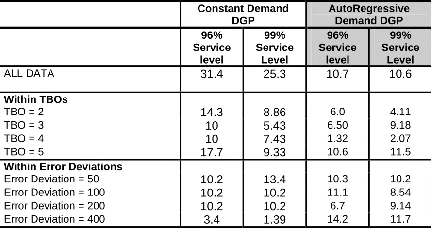
approximately follows a chi-squared distribution with k-1 degrees of freedom, where Ti is the sum of ranks for the ith lot size, so k = 6, and b is the number of factor levels, e.g., 16 if all TBOs 2 to 5 and error deviation values are considered, or 4 if only TBO or error deviation is considered. The values of the statistic are given in Table 2.
The χ2 values for 5 degrees of freedom with α = 0.1, 0.05 and 0.01 are 9.23, 11.07 and 15.08
[image:20.595.83.527.381.616.2]respectively. The values of the Friedman statistic in the first line of Table 2 indicate that overall there are significant differences in performance between the different lot sizing rules for the Constant Demand Process but for the Autoregressive Process, the p value is between 5% and 10%. An examination of the test statistics within TBOs (showing the variation in performance across error deviations) and within error deviations (showing the variation in performance across TBOs) shows somewhat more variation in performance across TBOs though the differences are not pronounced.
Table 2 - Dependency of Mean Unit Costs on Lot Sizing rule for Different TBOs and Error Deviations: (Friedman’s χ2 Test Statistics)
3
The use of common random numbers, while introducing dependence between unit costs for different treatments, does not undermine either Friedman’s test or the ANOVA tests considered later as the comparisons are blocked (as in a paired t-test).
Constant Demand
DGP AutoRegressive Demand DGP 96% Service level 99% Service Level 96% Service level 99% Service Level
ALL DATA 31.4 25.3 10.7 10.6
Within TBOs
TBO = 2 14.3 8.86 6.0 4.11
TBO = 3 10 5.43 6.50 9.18
TBO = 4 10 7.43 1.32 2.07
TBO = 5 17.7 9.33 10.6 11.5
Within Error Deviations
Error Deviation = 50 10.2 13.4 10.3 10.2
Error Deviation = 100 10.2 10.2 11.1 8.54
Error Deviation = 200 10.2 10.2 6.7 9.14
Another way to measure the relative performances is to calculate the ‘regret’ of using a particular lot sizing rule, the increase in unit cost compared to the best method for that TBO, error deviation and service level. Let Ci,j,k,l be the average unit cost for lot sizing rule i, using TBO j and error deviation k for service level l. The lowest unit cost is Mnj k l, , = Min Ci{ i j k l, , , }. Then the ratio
RC C Mn
Mn
i j k l
i j k l j k l j k l , , ,
, , , , ,
, ,
( )
= −
expressed as a percentage, is the cost regret of using the ith lot sizing rule for the TBO, error deviation
and service level compared to the lowest cost rule for that situation. The overall average regret values for each of the lot sizing rules for each service level for the Constant and Autoregressive Demand
DGPs are displayed in Table 3. This confirms the earlier deductions above.
It can be seen for the Constant Demand DGP that the EOQ rule always gives the best
performance by far for both service levels, with a regret of very close to 0%. The LUC rule is slightly better than POQ, LTC and SM rules, which are again slightly better than the WW rule. The size of the
regret falls as the error deviation increases and also as the TBO takes higher values. The potential saving in choosing the EOQ rule compared to any other is around 8% for a TBO of 2 but falls to only
1.4% for the highest TBO of 5, for the 96% service level. For the lowest error deviation the regret is
Table 3 - The Overall Average Percentage Regret by Error Deviation by Lot Sizing Rule. 3a) Constant Demand DGP
Service Level
Lot 96% 99%
Sizing Error Deviation Error Deviation
Rules 50 100 200 400 50 100 200 400
EOQ 0 0 0 0.075 0 0 0 0.05
POQ, 6.75 4.85 2.35 0.875 4.525 3.9 2 0.525
LUC 6.55 4.025 1.25 0.3 5.175 3.875 1.475 0.275
LTC 6.75 4.85 2.35 0.875 4.525 3.9 2 0.525
SM 6.75 4.85 2.35 0.875 4.525 3.9 2 0.525
WW 6.8 4.9 2.4 0.9 4.55 3.95 2.025 0.55
TBO TBO
2 3 4 5 2 3 4 5
EOQ 0.00 0.08 0.00 0.00 0.00 0.03 0.00 0.03
POQ, 8.43 2.88 2.08 1.45 5.85 2.05 1.73 1.33
LUC 5.90 3.33 1.80 1.10 4.80 2.93 1.80 1.28
LTC 8.43 2.88 2.08 1.45 5.85 2.05 1.73 1.33
SM 8.43 2.88 2.08 1.45 5.85 2.05 1.73 1.33
WW 8.43 2.88 2.08 1.63 5.85 2.05 1.73 1.45
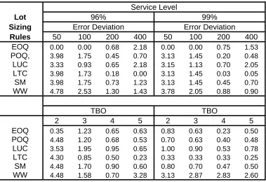
3b) Autoregressive (0.9) Demand DGP
Service Level
Lot 96% 99%
Sizing Error Deviation Error Deviation
Rules 50 100 200 400 50 100 200 400
EOQ 0.00 0.00 0.68 2.18 0.00 0.00 0.75 1.53
POQ, 3.98 1.75 0.45 0.70 3.13 1.45 0.20 0.48
LUC 3.33 0.93 0.65 2.18 3.15 1.13 0.70 2.05
LTC 3.98 1.73 0.18 0.00 3.13 1.45 0.03 0.05
SM 3.98 1.75 0.73 1.23 3.13 1.45 0.45 0.70
WW 4.78 2.53 1.30 1.43 3.78 2.05 0.88 0.90
TBO TBO
2 3 4 5 2 3 4 5
EOQ 0.35 1.23 0.65 0.63 0.83 0.63 0.23 0.50
POQ 4.48 1.20 0.68 0.53 0.70 0.63 0.40 0.48
LUC 3.53 1.95 0.95 0.65 1.00 0.90 0.53 0.78
LTC 4.30 0.85 0.50 0.23 0.33 0.33 0.33 0.25
SM 4.48 1.70 0.90 0.60 0.80 0.70 0.47 0.50
Comparing Table 3b with 3a shows that the regrets from using the best rule in each case is smaller for the Autoregressive DGP than from the Constant demand DGP. The EOQ is best for the
lower error deviations whilst the LTC rule is best for the two higher error deviations. The EOQ rule is best for a TBO of 2 but the LTC takes over for higher TBOs of 3, 4 or 5. The autoregressive results
show that generally the percentage regret from using the wrong rule is less than 2 %. Thus, unlike the Constant demand DGP, the choice of lot-sizing rule to use for the Autoregressive DGP is unimportant
except for very low error deviations and TBOs.
To summarise the results, for both processes, the choice of lot-sizing rule becomes less critical as the demand uncertainty increases, as the average time between orders increases and as the service
level increases and for higher TBOs and service levels is close to inconsequential.
It is also valuable to assess the increase in cost arising when forecasting uncertain demand
compared with the costs if future demand was known. This is illustrated in Table 4 where costs are
compared to those calculated with perfect foresight of the (stochastically) generated demand pattern for both DGPs. This shows the percentage increase in unit cost for the best lot sizing rule above the
unit cost for the corresponding WW cost based for the deterministic case of perfect foresight (disaggregated for the different TBOs and error deviations). The bottom row of the table shows the
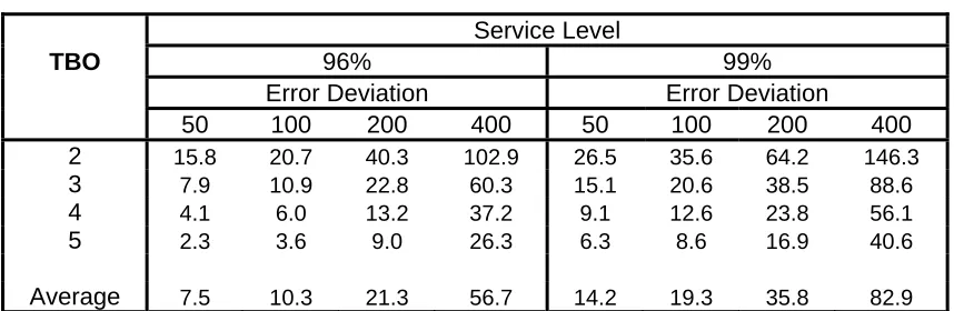
average increases over TBO values from 2 to 5. The increases are much higher for the 99% service level than for the 96% service level. The values derived indicate a complex pattern of behaviour, with
the standardised unit cost increase rising as the time between orders lengthens, the error deviation
increases and the service level incrases . There is again a significant difference between the two DGPs. The cost increases due to the uncertainty in the demand are much greater for the
Autoregressive DGP than for the Constant Demand DGP. The average of the 96% and 99% service levels can be used as an overall indicator of the effect of changes in the error deviation. The rate of
increase in unit cost as the error deviation increase is greater than a linear rate, but over the range given
is an increase of around 74% and 93% for every 100 units increase in the error deviation for the Constant Demand DGP and the Autoregressive DGP respectively.
These results contradict De Bodt and Wassenhove’s often repeated conclusion (1983a) that with any level of demand uncertainty greater than zero, costs were increased by about 10%. In fact,
this result is an artefact arising from the attempt to eliminate service level as a factor in the
Table 4 - The Percentage Increase in the Unit Cost of the Best LSR Rule Above the WW Solution based on Perfect Demand Information
4a) Constant Demand DGP
Service Level
TBO 96% 99%
Error Deviation Error Deviation
50 100 200 400 50 100 200 400 2 15.8 20.7 40.3 102.9 26.5 35.6 64.2 146.3
3 7.9 10.9 22.8 60.3 15.1 20.6 38.5 88.6
4 4.1 6.0 13.2 37.2 9.1 12.6 23.8 56.1
5 2.3 3.6 9.0 26.3 6.3 8.6 16.9 40.6
Average 7.5 10.3 21.3 56.7 14.2 19.3 35.8 82.9
4b) Autoregressive (0.9) Demand DGP
Service Level
TBO 96% 99%
Error Deviation Error Deviation
50 100 200 400 50 100 200 400 2 18.3 31.1 71.4 180.0 31.7 51.6 106.6 243.2
3 9.1 15.9 38.0 108.1 17.6 29.1 60.6 150.6
4 4.6 8.5 22.7 67.7 10.6 17.4 37.8 97.1
5 2.7 5.5 15.4 48.1 7.2 12.4 27.1 69.9
Average 8.7 15.3 36.9 101.0 16.8 27.6 58.0 140.2
6. THE VALUE OF FORECASTING and THE EFFECTS OF MISSPECIFICATION
Now the above results are indicative of the value of forecasting. Transparently, changes in the demand uncertainty leads to significant changes in the unit cost when service level is kept fixed.
However, this does not directly answer the question posed in the introduction: what is the value of forecasting. To most practitioners, the forecast error is the difference between the actual and the
forecast value. However, this error combines the randomness in the process generating the demands and the errors arising from not using the optimal forecast and most earlier researchers in this area have
conflated the two. It is only the latter that represents the potential value of improving forecasting accuracy. Our analyses to date have assumed the use of the optimal forecasting method. The
non-optimal forecasting system cans now be defined as:
t k t t opt k t
t F
F−1,+ = −1,+ +ν
(assuming the same error is made across lead times). It follows that the overall forecast error is
t k t k t t k
t F e
D+ − −1,+ = + −ν
This distinction between randomness in the data generation process and the consequential
forecasting errors permits the introduction of a wide range of forecasting error characteristics, including bias and forecast model specification error. However, in this paper we only examine the
case where νt has error standard deviation κσ where κ is chosen so that the overall error deviation,
σ√(1+κ2), takes values of 110%, 120% and 150% of the minimum attainable, given by σ. The results
from introducing forecast error should look similar to those just presented for different levels of
randomness in the data generation process alone despite the two sources of error being independently
simulated. (This will not in general be true in the common case where etand νt are correlated.)
There are thus two sources of uncertainty in the demand prediction process. One, the
forecasting error, can be reduced by getting closer to the optimal forecasting method for the underlying demand generation process (DGP). Clearly, as there will be inevitable errors in identifying and
estimating the parameters of the DGP, it will never be possible to eliminate such forecasting errors altogether. The second source, the process error deviation, is the random variation in the DGP itself.
This can be reduced only by attempting to manage the demand process, for example by attempting to change customers’ behaviour or through collaborative forecasting. The use of specific ordering days in
a week or month for different groups of customers in inventory/distribution systems offers an
illustration. It is important in guiding management effort towards process improvements to distinguish
as much as possible between the impact of these two sources of uncertainty on unit costs and service level.
Figure 2 shows the effects on the unit cost / service level trade-off curves of increasing the
forecasting error by 20% and 50% compared to when the forecast is optimal (i.e. νt.≡0). This is further
contrasted with the curve based on perfect foresight information. The illustrative graph of the results shown is derived using the EOQ lot sizing rule and for a TBO of 3 periods for different standard
Figure 2: Unit Cost vs Service Level as it is affected by Forecast Error Levels
Based on the EOQ: Time Between Orders 3 Periods
Demand Uncertainty = 100 Demand Uncertainty = 400
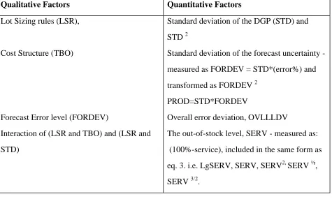
In order to quantify the value of forecasting, the logarithm of unit costs has been modelled as a function of possible explanatory factors as given in Table 5. As before, the model was of log(average unit cost). The data set modelled was for mean service levels lying between 93% and 99.9% to avoid distortions at the extremes of the data matrix. This range includes those values of practical interest.
Table 5 Possible Explanatory Factors in a Model of Lge(Cost)
In the model specification the service level has been included in the same form as was used to
Qualitative Factors Quantitative Factors
Lot Sizing rules (LSR), Standard deviation of the DGP (STD) and
STD 2
Cost Structure (TBO) Standard deviation of the forecast uncertainty - measured as FORDEV = STD*(error%) and
transformed as FORDEV 2 PROD=STD*FORDEV
Forecast Error level (FORDEV) Overall error deviation, OVLLLDV Interaction of (LSR and TBO) and (LSR and
STD)
The out-of-stock level, SERV - measured as:
(100%-service), included in the same form as eq. 3. i.e. LgSERV, SERV, SERV2, SERV ½,
[image:26.595.71.546.399.684.2]estimate the 99% and 96% service levels in section 5. The results show that the factors LSR and Cost (as measured by TBO) are significant. Perhaps unsurprisingly, the largest reduction in variance is due
to the Cost (TBO) parameter. The standard deviation of the data generation process, STD, and the forecast error deviation, FORDEV, were included linearly. The inclusion of the variances, STD2 and
FORDEV2, as well as the standard deviations led to improved predictions for the larger values of the overall deviation (OVLLLDV). The RMSE is low suggesting a satisfactory model (with interquartile
ranges of approximately ±5% for the error) with R2 of 99%. Details of the associated analysis of variance summary table are omitted as the inevitable consequence of using such a large data set is almost all factors were found to be ‘significant’.
Graphical analysis plus the inclusion of additional cross-product terms such as the often
insignificant interactions between OVLLLDV and LSR and TBO suggested that the model was broadly adequate and the error distribution was approximately normal but it failed to capture all the
non-linearities induced by the interaction of STD, the standard deviation of the DGP, and the cost structure, TBO. However, including such interaction terms had no effect on the qualitative
conclusions we draw and little effect on the quantitative estimates we make since the coefficients are
small. The final specification adopted included a dummy variable to distinguish between the situation
with zero forecast error deviation (FORDEV=0) and non-zero forecast error. Its interaction with LSR was also included.
The key interaction to include is that between the cost parameter and the overall uncertainty
(OVLLLDV), preferred to both the process standard deviation (STD) or the forecast error deviation (FORDEV). This shows that the impact of the overall deviation lessening as the time between orders
(TBO) increases. Essentially the shorter the time between orders the more sensitive the system is to
uncertainty and forecast error. The impact of the forecast error deviation is larger, compared to the process error though there is a qualitative reduction in cost in moving from the zero forecast error deviation to the non-zero case, i.e small amounts of forecast error lead to overall improvements in
performance.
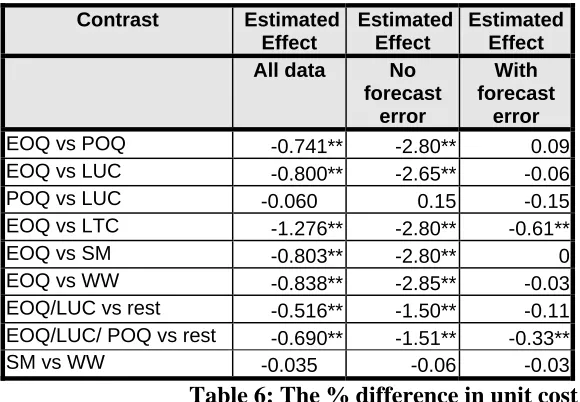
The above model was used to evaluate the performance of the different lot sizing rules, see Table 6.
results disguises a more complex picture that becomes apparent if the analysis is carried out only for those points with zero forecast error deviation on the one hand and positive deviation on the other.
While overall EOQ is not the uniform best performer, for zero forecast error deviation it is
significantly better than its competitors (confirming table 1 and 3) whilst the best performers with
[image:28.595.111.401.238.439.2]forecast error were EOQ, POQ and LUC which differed significantly from the rest. Whatever the error deviation, there was no significant difference found between Silver-Meal and Wagner-Whitin.
Table 6: The % difference in unit cost:
Testing the difference between Lot Sizing Rules - the Contrasts (** represents a contrast significant at less than 1%)
Estimating the value of forecasting requires some assumptions about the size of the overall uncertainty that arises in practice and also how it is divided between the noise in the process
generating demand and the forecast errors incurred from using a non-optimal forecasting method. Only the second source of error is lessened by improved forecasting. It was stated in section 2 that, in
practice for short term forecasting, weekly or monthly up to three steps ahead, the standard error of the forecast for faster moving items would usually not typically exceed 40% of the mean demand (i.e. a
value of 400 if the mean demand was 1000). Improvements in forecasting of around 20-50% in the overall forecast error are possible by implementing appropriate forecasting techniques to match the
particular characteristics of the demand data used in the MRP system (Fildes et al, 1998, Fildes et al, 2004). Thus, it would be indicative of possible savings in unit cost to consider the improvements
Contrast Estimated Effect
Estimated Effect
Estimated Effect All data No
forecast error
With forecast
error
expected for values of 200 and 400 in the overall uncertainty, derived from different mixes in process noise and forecast error. Using the above response model specification, the estimated % change in
cost is independent of cost, LSR and service level. Using a first order approximation for the response function the percentage improvement in unit cost for an h% improvement in forecasting accuracy is
given by:
h FORDEV STD
FORDEV OVLLDV
FORDEV
prod fordevsq
fordev OVLDV
TBO, β 2β β )* *
β + + +
where FORDEV is the forecast error, and OVLLLDV is the overall uncertainty. The β coefficients have the obvious meaning with βTBO, OLVLLDV representing the interaction term. In quantitative terms
βfordev dominates the improvement from improved accuracy but the formula shows the size of the
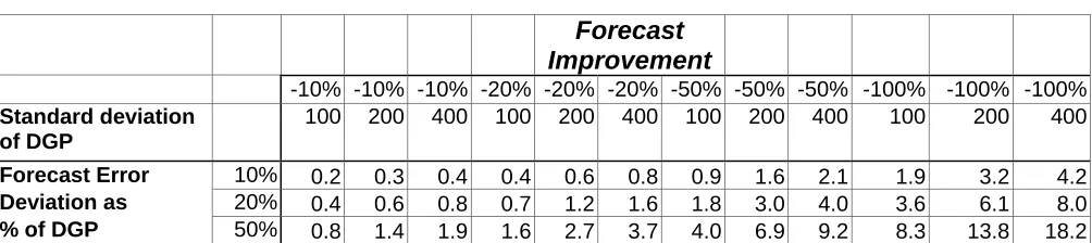
forecast error is also critical. Illustrative exact results are shown in Table 7 for EOQ. The
approximation underlines the importance of the forecast error deviation relative to the process noise. In effect major improvements in cost can be achieved where the overall uncertainty is high and a major
[image:29.595.57.559.520.632.2]component of this is forecast error. However, the table also highlights the difficult of making such gains.
Table 7a. The Value of Forecasting for Different % Improvements in Forecasting Error
– the % reduction in Unit Costs for the AR(0) process (averaged over TBO) Forecast
Improvement
-10% -10% -10% -20% -20% -20% -50% -50% -50% -100% -100% -100%
Standard deviation of DGP
100 200 400 100 200 400 100 200 400 100 200 400
Forecast Error 10% 0.2 0.3 0.4 0.4 0.6 0.8 0.9 1.6 2.1 1.9 3.2 4.2
Deviation as 20% 0.4 0.6 0.8 0.7 1.2 1.6 1.8 3.0 4.0 3.6 6.1 8.0
% of DGP 50% 0.8 1.4 1.9 1.6 2.7 3.7 4.0 6.9 9.2 8.3 13.8 18.2
The final stage in this analysis of the value of forecasting is to analyse the results obtained for the second autoregressive generating process through the analysis of variance. The model had the same characteristics as that for constant demand (although some slight improvement could have been
obtained by using the interaction between TBO and the forecast uncertainty). The estimated
Because of the greater interdependence of LSR and cost structure, unlike the simple constant demand model, there is no simple equivalence between the results of the analysis of contrasts and the ranking
results in Table 1.
Table 7b. The Value of Forecasting for Different % Improvements in Forecasting Error
– the % reduction in Unit Costs for the AR(.9) process (averaged over TBO) Forecast
Improvement
-10% -10% -10% -20% -20% -20% -50% -50% -50% -100% -100% -100%
Standard deviation of DGP
100 200 400 100 200 400 100 200 400 100 200 400
Forecast Error 10% 0.2 0.3 0.4 0.3 0.6 0.8 0.8 1.4 2.0 1.5 2.7 3.9
Deviation as 20% 0.3 0.6 0.8 0.7 1.2 1.7 1.6 2.8 4.1 3.1 5.4 7.8
% of DGP 50% 0.9 1.6 2.3 1.9 3.2 4.5 4.5 7.7 10.7 8.2 14.0 19.4
An alternative approach to the problem of estimating the value of improved forecasting
accuracy is by using the raw simulation results and comparing the unit cost of dropping from 50% forecast error to 20% to 0% for fixed service (at 96% and 99%). This approach gives a higher
estimates of the forecast sensitivity, with median forecast sensitivity of 10% at the 96% service level (17% at 99%) and 11% at 96% service (20% at 99%) at process standard deviations of 200 and 400
process uncertainty respectively. Interestingly a small amount of forecast error and low process uncertainty resulted in a small cost improvement. For the AR(.9) process the effects of forecasting
improvement are uniformly larger with approximate unit cost improvements of 5% and 8% above the AR(0) benchmark values given above.
Misspecification
In applications, simple forecasting methods are usually applied without any prior analysis of the appropriate underlying mode of the DGP. The effect is to introduce both forecast error and
misspecification error. As noted in the introduction such misspecification is a common feature of various supply chain models discussed in the literature including most recently Chen et al, 2000a and
Zhao et al, 2001. A full discussion of its effects of misspecification would ensure the paper was overly long. However, we have considered two cases, where the DGP is the constant demand model and the
levels and lot-sizing rules EOQ, POQ and LTC which ensured the ‘better’ LSRs have been used.
Data Generating Process
AR(0) AR(.9)
Forecast Noise: Mean Mean
AR(0) 00% 15.4% 46.1%
20% 26.4% 50.0%
50% 39.3% 54.8%
AR(.9) 0 25.6% 25.1%
Forecasting Generating Process
20% 67.6% 46.7%
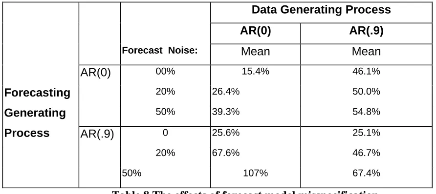
[image:31.595.54.500.121.320.2]50% 107% 67.4%
Table 8 The effects of forecast model misspecification
(averaged over the ‘better’ lot sizing rules, EOQ, POQ and LTC, averaged over TBOs 3 &4, for process uncertainty of 100 and 200 and service levels).
The table illustrates the effects of using a mis-specified model (typically the case in previous research)
compared with using an optimal model for the particular case. The table is split into four quadrants, the first under the heading AR(0) repeats the unit cost where the DGP is an AR(0) process and the optimal
forecasting model specification has been used to model the DGP (but with three levels of forecast error, 0% 20% and 50%, of the demand uncertainty). The fourth quadrant shows the results where the
DGP is again the AR(0) but the forecasting model that is used is AR(.9) (again with the three levels of noise). Quadrants two and three are similar but the DGP is AR(.9). The results strongly confirm the
lack of symmetry in the two specification errors – a greater percentage error is incurred by assuming the process is AR(0) if in fact it is AR(.9) than vice versa but only when the forecast error noise is
around 20% or lower – i.e. no dominant strategy is available for selecting a forecasting model. In addition, an analysis of the more detailed results show the specification error effects on costs increases
with TBO, process uncertainty and service level. No differences in performance were observed for these ‘better’ performing lot sizing rules. Thus, earlier research (which makes assumptions equivalent
to mis-specifying the forecasting model adopted in the simulation) is likely to have misstated the effects of demand uncertainty, potentially substantially, and their conclusions will be dependent on the
7. DISCUSSION and CONCLUSIONS
In this research we have demonstrated a methodology for integrating aspects of manufacturing research with forecasting. The methodological issues we have explored aimed to highlight deficiencies
in previous research designs: the conflation of demand uncertainty with forecasting error uncertainty and model mis-specification, the use of 100% service levels to draw conclusions and the pervasive use
of Analysis of Variance when the issue of significance can easily be dealt with through increased sample size, thus neglecting the much more fundamental issue of the practical importance of the results. Size matters! (Zilian and McCloskey, 2004). The substantive aim of the research has therefore
been to show how to estimate the value of improved forecasting and to flesh out the claims made by
software suppliers and forecasters alike that accurate forecasting is critical to many manufacturing operations
Various stylised facts spring from the substantive analysis we have presented.
• Unit cost (expressed as a percentage of the unit cost based on perfect foresight) increases
exponentially with demand uncertainty in contrast to de Bodt’s and Van Wassenhove’s (1983a) assertion. The discrepancy with this study apparently arises from their focus on service levels of 100% only.
• In the more general framework established here, the best lot sizing rules when demand
uncertainty exists remain very different to those based on deterministic demand which assumes perfect foresight. This strengthens, for example, Wemmerlov and Whybark, (1984),
− A possible explanation of the relative performance of the various lot sizing rules is that for a