Analytical Solution of Substrate Concentration in the Biosensor Response

http://dx.doi.org/10.4236/am.2013.412217

Analytical Solution of Substrate Concentration in the

Biosensor Response

Seyed Ali Madani Tonekaboni1, Ali Shahbazi Mastan Abad2, Amin Afshari2, Ali Khalilzadeh2, Shahab Karimi2, Mitra Shabanisamghabady2

1

School of Mechanical Engineering, University of Waterloo, Waterloo, Canada

2

School of Mechanical Engineering, University of Tehran, Tehran, Iran

Email: [email protected], [email protected], [email protected], [email protected], [email protected], [email protected]

Received September 8, 2013; revised October 8, 2013; accepted October 15, 2013

Copyright © 2013 Seyed Ali Madani Tonekaboni et al. This is an open access article distributed under the Creative Commons Attri- bution License, which permits unrestricted use, distribution, and reproduction in any medium, provided the original work is properly cited.

ABSTRACT

Homotopy analysis method (HAM) is employed to investigate amperometric biosensor at mixed enzyme kinetics and diffusion limitation. Mathematical modeling of the problem is developed utilizing non-Michaelis-Menten kinetics of the enzymatic reaction. Different results of the problem are obtained for different values of the dimensionless parameters. Accuracy of the obtained results is verified by comparing them with the available actual and simulated ones. It is con- cluded that the obtained solution can be considered as a promising one to investigate different aspects of the phenom- ena.

Keywords: Homotopy Analysis Method; Amperometric Biosensor; Mathematical Modeling; Non-Michaelis-Menten Kinetics

1. Introduction

Biosensors play important roles as components of the transduction mechanisms [1] and can be employed as measurement devices to gauge biologically relevant in- formation such as neural interfaces and oxygen elec- trodes [2]. Furthermore, they can be used as transducers which translate the biomolecular responses into electrical signals [3]. Biosensors produce signals harmonized to the concentrations of the measured analytes. These devices are used in so many applications like detection of patho- gens [4], toxic metabolites (such as mycotoxins [5]), de- tection of pesticides and river water contaminants such as heavy metal ions [6], etc. The mentioned examples show the importance of biosensors and their applications in different branches of Science and Engineering which reveals the requirement of analysis of these highly de- manded instruments. One of the popular and perspective trends of biosensorics is amperometric biosensor [7]. Since they were first introduced by Clark and Lyons in 1962 [8], several studies have investigated different as- pects of amperometric biosensors. In principle, they measure the changes of the current of indicator electrode

by direct electrochemical oxidation or reduction of the products of the biochemical reaction [9-11]. They are widely used today because of the reliability and high sensitivity for environment, clinical and industrial appli- cations.

Design of biosensors is based on understanding the kinetic characteristics of these devices. Generally, meas- uring the concentration of substrate inside enzyme mem- branes is not possible. Hence, various mathematical models of amperometric biosensors have been presented and used as an important tool in order to obtain analytical characteristics of actual biosensors [12,13], such as in- vestigative monolayer membrane model used to study the biochemical treatment of biosensors [14,15]. Their ma- thematical models are based on reaction-diffusion equa- tions including non-linear term that relate to non-Micha- elis-Mentenkinetics of the enzymatic reaction [16,17]. Hence, high accurate analytical and numerical methods should be employed to investigate this important nonlin- ear chemical equation.

Therefore, the constitutive laws of these problems should be solved using other schemes such as numerical or per- turbation methods. In the numerical method, stability and convergence of the solution should be considered so as to avoid divergence or inappropriate results [18]. In the perturbation method, the small parameter is inserted in the equation; thus, finding the small parameter and ex- erting it into the equation is one of the deficiencies of this method [19]. One of the semi-exact methods for solving nonlinear equation which does not need small/large pa- rameters is Homotopy Analysis Method (HAM), first proposed by Liao [20,21]. Homotopy Analysis Method is now widely used to solve different types of nonlinear problems. Various papers on nonlinear physical and en- gineering problems [22,23] have proved the validity of HAM. Moreover, recently the application of HAM on medical and chemistry problems has gotten so much at- tention among researchers. Counting reaction network equilibria [24], reaction-diffusion Brusselator model [25], predicting the lowest energy conformations of proteins [26] and many other examples can be considered as ap- plications of HAM in Chemistry and Medicine. Several auxiliary parameters and functions available in the pro- cedure of HAM need to be chosen so properly for the convergence of the solution. Through practice of auxil- iary parameter h, convergence region of the solution is readily adjustable to a wide range of variables.

This paper presents the analytical solution for an am- perometric biosensor at mixed enzyme kinetics and dif- fusion limitation by utilizing HAM as a strong method. Non-Michaelis-Menten kinetics of the enzymatic reac- tion is used to obtain the constitutive equation of the problem. Different non-dimensional parameters are de- fined so as to non-dimensionalize the equation. The ob- tained non-dimensional equation is used to procure mth-

order deformation equation as an important step of the procedure of the solution. The h-curves are obtained for several cases illustrated in the paper to clarify the con- vergence region of the solution. In addition, results are obtained to investigate the effects of the variations of each dimensionless parameter of the procured equation. Finally, some of the results are compared with the actual and simulated results available in the literature [27] to verify the accuracy of the method.

2. Mathematical Modeling

Spatial dependency of enzyme kinetics on biochemical systems has recently attracted much attention by consid- ering the effect of diffusion in these processes [16,17]. The simplest scheme of non Michaelis-Menten kinetics may for instance be described by adding to the Micha- elis-Menten scheme (2.1) the relationship of the interact- tion of the enzyme substrate complex



with an-

other substrate molecule



ES

 

S

ES

(2.2) followed by the gen- eration of non-active complex



ES2 as

E P



E S  

S



2

ES

(2.1)

ES 



(2.2)

The reaction is sometimes said to display Michaelis- Menten kinetics in which the relationship between the rate of an enzyme catalyzed reaction and the substrate concentration takes the form



 

max

M

V S

K S (2.3)





where  and Vmax are the so-called “initial reaction

velocity” and maximum velocity respectively.

In addition, KM is known as Michaelis constant for

.

S KM and Vmax are constants at a given temperature

and a given enzyme concentration.

The reactions exhibit non-Michaelis-Menten kinetics, in which the kinetic behavior does not obey the Equation (2.3). The velocity function  for the simple reaction process without competitive inhibition is given by Pao [28] and Baronas et al. [27], which is based on the non- Michaelis-Menten hypothesis,

   

   

   

 

max 0

2 2

c

M i M i

k E S V S

K S S K S K

 

  K  S 



(2.4)

where the constants _max



0 c

V k E , K_M and K_i are Michaelis-Menten and inhibition constants respectively. The Equation (2.4) conforms to Equation (2.3) for large values of Ki with respect to KM . On the basis of

Equation (2.4), the rate is maximized by increasing the concentration. It is then said to be inhibited by the sub- strate. In addition, the constant Ki (which has the di-

mension of a concentration) is called the substrate inhibi- tion constant. For obtaining the rate of change of sub- strate concentration S S

 

,t at time t and position

  throughout the domain, the following equation given by Pao [28] is used.

  

,



S

S _{D S t}

t  



   

 (2.5)

S is the substrate diffusion coefficient and

D S is

the gradient operation. On the basis of non-Michaelis- Menten kinetics, Equation (2.5) becomes

2

2 2

1

S

M i M

S _D S S

t  S K K K

 

 

  

K S

 (2.6)

in which K K E Kc 0 M . In this article, steady state

2

2 2 0

1

S

M i M

S KS

D

S K S K K

 

 

   (2.7)

Equation (2.7) is changed to the non-dimensional form (Equation (2.8)) [27] using the following non-dimen- sional parameters

2

2 2

2 2

0, 0 1

1

, , , ,

S M

u Ku _u

x u u

S kL ks

u x K

L D K K K

ks    _{ }  _    _{   }          i M ks (2.8)

Equation (2.8) must be solved to satisfy the following boundary conditions which are based on the location of electrodes and diffusion layer in the boundaries of the membarne

1 at 1

0 at 0

u x u x x    _{ }  (2.9)

3. HAM Solution

In this section the solution procedure of this problem using HAM is discussed. The appropriate form of non- linear differential Equation (2.8) for the procedure of HAM is presented as follows:

 



 



 





 





 

2 2 2

, 1 , ,

, , 0

N x q x q x q

x q K x q x               _{ }  (3.1)

where _{is the node number,} is the nonlinear op- erator, and the function

i

N

 

i q

 is defined as

 

 

 

 

0 0

1

lim , ,

lim ,

q

q

x q u x x q u x

 







 (3.2)

where u x

 

is the unknown field variable, q

 

0,1

is the embedding parameter, and is the initial guess which is employed to meet the requirements of the boundary conditions. In this paper, the

 

0

u x

 

0

u x 1 has been chosen which correctly satisfies all the boundary conditions stated in Equation (2.9).

So through the generalizing concept of HAM the so- called zero-order deformation equation can be written as:



1q L





 

x q, u x0

 

qhH x N

 



 

x q,  (3.3)

where h0 is the non-zero auxiliary parameter,

 

H x is the auxiliary function, and is the auxiliary linear operator which is chosen here as

L

 





2

 

2

d d f x f x x 

 (3.4)

with the following property:



C1xC2



0 when C1xC2 0

  (3.5)

Expanding 

 

x q, in Taylor series with respect to the embedding parameter

q

, one obtains

 

 

 

 

 

0 1 0 , , 1 ! m m m m m m q

x q u x u x q

x q u x m q          



(3.6)

With due attention to the procedure of HAM [21],

 

m

u x should be chosen so as the following equation is satisfied

 

0 d 1 0 d m m X u u X 

  (3.7)

If the series 

 

x q, converges at , then the se- ries solution is

1

q

 

0

 

 

1

,1 _m

m

x u x u x

 



 



(3.8) where um

 

x could be obtained by the so-called high-

order deformation equation. For obtaining the mth-order

deformation equation, the following vector is defined as:

   

 



0 , 1 , ,



n u x u x  u x

u _n (3.9) Differentiating both sides of the zero-order equation m times with respect to and then setting , the so- called mth-order deformation equation can be obtained as

q q0

 

1

 

 



1,

m m m m m

L u x  u  x hH x R u  x



(3.10)

where

0, 1 1, otherwise

m

m

   

 (3.11)



1

_{  }

1

 

1

0 , 1 , 1 ! m

m m m

q

N x q

R x m q       _ _   

u (3.12)

Therefore, the following relation is obtained





1

1 1 0 1 1 1 0 0 , m

m m m i m i

i

m i

m i k i k m

i k

R x u u u

u u u Ku

   1                   







u  (3.13)

We are free to choose the auxiliary parameter , the auxiliary function

h

 

H x , the initial guess 0

 

x , and

the auxiliary linear operator so that the validity and flexibility of the HAM solution to control the conver- gence region is proven. Due to the rule of solution ex-

pression [21] the auxiliary function is chosen as follows

u L

 

1

iary parameter h for convergence of the solution series is the flat regions of h-curves.

4. Results and Discussion

To see the proper values of h, the h-curves are plotted for different values of dimensionless parameters

, and K

  in Figure 1 to obtain the valid results of the considered conditions.

Figure 1. Variations of u x

 

, β 0



versus non-dimensional pa-

ramete for (a) ; (b) , ; (c)

; and (d) .

x

,



1.0 .1

α 

10.0

α

0.1 1.0

α β

1.0

β

10.0 0.1

α β  , 

The procedure of solving the non-dimensional equa- tion of enzyme reaction (Equation (2.8)) which is based on the non-Michaelis-Menten kinetics theory utilizing HAM is described in Section 3. It is mentioned that

mth_{-order deformation}

equation should be employed to solve the problem. As the first step of the solution, the diagrams of variation of non-dimensional parameter

 

u x versus auxiliary parameter h for different investi- gated cases are illustrated (Figure 1). Then, flat regions of h-curves are obtained employing these diagrams.

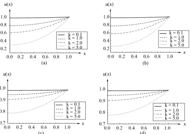
On the basis of the chosen values of auxiliary parame- ter h in the flat regions of h-curves (Figure 1)the varia- tions of u x

 

versus x _{were examined (}Figure 2) to clarify the dependency of these variations on different non-dimensional parameters defined in Equation (2.8).

Figure 2 clearly demonstrates that the effect of variation of non-dimensional parameter K on the profiles of u x

 

is so important which causes large differences between values of u x

 

for different values of K. Values of

 

u x at different locations are presented in Table 1 and

Table 2 for better clarifying the effects of K as well as other non-dimensional parameters



 ,



.

Table 1. Values of non-dimensional variable u x

 

1.0

β

at dif-

ferent locations for α1.0, ,β0.1,α0.1  K

and for different values of non-dimensional parameter .

x α = 1.0, β = 0.1 α = 0.1, β = 1.0

K = 0.1K = 1.0K = 2.0K = 5.0 K = 0.1 K = 1.0 K = 2.0K = 5.0

0 0.9764 0.7831 0.6095 0.3012 0.9762 0.7675 0.5697 0.2517

0.2 0.9773 0.7916 0.6264 0.3245 0.9771 0.7767 0.5862 0.2517

0.4 0.9802 0.8172 0.6695 0.3971 0.9800 0.8044 0.6362 0.3515

0.6 0.9849 0.8601 0.7458 0.5261 0.9848 0.8507 0.7209 0.4885

0.8 0.9915 0.9209 0.8551 0.7225 0.9914 0.9159 0.8417 0.7002

1.0 1.0000 1.0000 1.0000 1.0000 1.0000 1.0000 1.0000 1.0000

Table 2. Values of non-dimensional variable u x

 

at diferent locations for α10.0, β0.1,

and for different values of non-dimensional parameter . , 1

α β

K

10.0 .0

x α = 10.0, β = 0.1 α =10.0, β = 1.0

K = 0.1K = 1.0K = 2.0K = 5.0 K = 0.1 K = 1.0 K = 2.0K = 5.0

0 0.9955 0.9551 0.9105 0.7795 0.9958 0.9583 0.9167 0.7927

0.2 0.9957 0.9569 0.9141 0.7882 0.9960 0.9600 0.9200 0.8010

0.4 0.9962 0.9623 0.9248 0.8146 0.9965 0.9650 0.9300 0.8258

0.6 0.9971 0.9712 0.9427 0.8586 0.9973 0.9733 0.9467 0.8672

0.8 0.9984 0.9838 0.9678 0.9204 0.9985 0.9850 0.9700 0.9253

5. Conclusion

Verification of the Solution

In order to verify the accuracy of the obtained solution, results are compared with available simulation and exact solutions available in the literature [28] for the special case of  0, 0 (Table 3). It is shown that the values of the results of HAM and exact solution in the considered special case are identical to each other at the considered numerical precision. It should be noted that exact solutions are available only for this special case. The excellent agreements between HAM and exact solu- tions in Table 3 suggest that HAM can yield highly ac- curate solutions not only for the special cases but also for the general cases for which exact solution does not exist. Hence, the results presented in this paper can be utilized as promising data for investigating the behavior of the general enzyme reaction.

Analytical solution of the amperometric biosensor at mixed enzyme kinetics and diffusion limitation is pre- sented utilizing HAM. Dimensionless equation of the problem is obtained using the mathematical modeling presented in the paper which is based on non-Micha- elis-Menten kinetics of the enzymatic reaction. Solution procedure of the non-dimensional equation of enzyme reaction is described and mth-order deformation equation is obtained on the basis of the non-dimensional enzyme reaction equation presented in this article. Several

[image:5.595.143.454.296.515.2]

h-curves are presented to show the convergence region of the solution. Results of the solution are presented for different quantities of the dimensionless parameters used to non-dimensionalized the enzyme reaction equation. It is clarified that the most effective parameter in the reac-

Figure 2. Variations of u x

 

versus auxiliary parameter x for (a) α1.0, β0.1 ; (b) ; (c)

; and (d) .

,

0.1 1.0

α β

,

10.0 0.1

α β α10.0, β1.0

Table 3. Comparison of the results of the HAM with simulation and actual results of the problem at different locations and for different values of non-dimensional parameter K



α0, β0



.

K = 0.1 K = 1.0 K = 5.0

x Simulation HAM Exact Simulation HAM Actual Simulation HAM Actual

0 0.9500 0.9520 0.9520 0.6500 0.6481 0.6481 0.2100 0.2113 0.2113

0.25 0.9529 0.9550 0.9550 0.6666 0.6684 0.6684 0.2502 0.2452 0.2452

0.50 0.9613 0.9639 0.9639 0.7293 0.7303 0.7303 0.3585 0.3578 0.3578

0.75 0.9767 0.9789 0.9789 0.8366 0.8390 0.8390 0.5893 0.5851 0.5851

1.0 0.9976 1.0000 1.0000 0.9940 1.0000 1.0000 0.9970 1.0000 1.0000

[image:5.595.57.540.597.735.2]

tion and local dependency of the dependent variable of the problem u x

 

is K. Conclusively, some available results in the literature are used to prove the high accu- racy of the presented solution.

REFERENCES

[1] F. Scheller and F. Schubert, “Biosensors,” Elsevier, Am- sterdam, 1988.

[2] U. Wollenberger, F. Lisdat and F. W. Scheller, “Enzy- matic Substrate Recycling Electrodes,” Frontiers in

Bio-sensorics II, Vol. 81, 1997, pp. 45-70.

[3] M. Pohanka, P. Skladal and M. Kroca, “Biosensors for Biological Warfare Agent Detection,” Defense Science Journal, Vol. 57, No. 3, 2007, pp. 185-193.

[4] M. Pohanka, D. Jun and K. Kuca, “Mycotoxin Assay Using Biosensor Technology: A Review,” Drug and Che-

mical Toxicology, Vol. 30, No. 3, 2007, pp. 253-261. http://dx.doi.org/10.1080/01480540701375232

[5] S. Haron and A. K. Ray, “Optical Biodetection of Cad- mium and Lead Ions in Water,” Medical Engineering and

Physics, Vol. 28, No. 10, 2006, pp. 978-981. http://dx.doi.org/10.1016/j.medengphy.2006.04.004

[6] A. J. Baeumner, C. Jones, C. Y. Wong and A. Price, “A Generic Sandwich-Type Biosensor with Nanomolar De- tection Limits,” Analytical and Bioanalytical Chemistry, Vol. 378, No. 6, 2004, pp. 1587-1593.

http://dx.doi.org/10.1007/s00216-003-2466-0

[7] K. R. Rogers, “Biosensors for Environmental Applica- tions,” Biosensors and Bioelectronics, Vol. 10, No. 6-7, 1995, pp. 533-541.

http://dx.doi.org/10.1016/0956-5663(95)96929-S

[8] A. P. F. Turner, I. Karube and G. S. Wilson, “Biosensors: Fundamentals and Applications,” Oxford University Press, Oxford, 1987.

[9] U. Wollenberger, F. Lisdat and F. W. Scheller, “Frontiers in Biosensorics 2. Practical Applications,” Birkhauser Verlag, Basel, 1997.

[10] A. Chaubey and B. D. Malhotra, “Mediated Biosensors,”

Biosensors and Bioelectronics, Vol. 17, No. 6-7, 2002, pp. 441-456.

http://dx.doi.org/10.1016/S0956-5663(01)00313-X

[11] G. G. Guilbault and G. Nagy, “An Improved Urea Elec- trode,” Analytical Chemistry, Vol. 45, No. 2, 1973, pp. 417-419. http://dx.doi.org/10.1021/ac60324a053

[12] L. D. Mell and J. T. Maloy, “A Model for the Am- perometric Enzyme Electrode Obtained through Digital Simulation and Applied to the Glucose Oxidase System,”

Analytical Chemistry, Vol. 47, No. 2, 1975, pp. 299-307. http://dx.doi.org/10.1021/ac60352a006

[13] J. D. Hoffman, “Numerical Methods for Engineers and Scientists,” McGraw-Hill, New York, 1992.

[14] T. Schulmeister, “Mathematical Modeling of the Dy- namic Behavior of Ampero-Metric Enzyme Electrodes,”

Selective Electrode Reviews, Vol. 12, 1990, pp. 203-260. [15] R. Aris, “The Mathematical Theory of Diffusion and Re-

action in Permeable Catalysts: The Theory of the Steady State,” Clarendon Press, Oxford, 1975.

[16] L. K. Bieniasz and D. Britz, “Recent Developments in Digital Simulation of Electroan-Alytical Experiments,”

Polish Journal of Chemistry, Vol. 78, 2004, pp. 1195- 1219.

[17] S. J. Liao, “Beyond Perturbation: Introduction to the Homotopy Analysis Method,” Chapman and Hall/CRC Press, Boca Raton, 2003.

http://dx.doi.org/10.1201/9780203491164

[18] A. H. Nayfeh, “Problems in Perturbation,” 2nd Edition, Wiley, New York, 1993.

[19] S. J. Liao, “The Proposed Homotopy Analysis Technique for the Solution of Nonlinear Problems,” Ph.D. Thesis, Shanghai Jiao Tong University, Shanghai, 1992.

[20] P. Manimozhi, A. Subbiah and L. Rajendran, “Solution of Steady-State Substrate Concentration in the Action of Biosensor Response at Mixed Enzyme Kinetics,” Sensors

and Actuators B, Vol. 147, No. 1, 2010, pp. 290-297. http://dx.doi.org/10.1016/j.snb.2010.03.008

[21] S. Abbasbandy, T. Hayat, “Solution of the MHD Falkner- Skan Flow by Homotopy Analysis Method,” Communi-

cations in Nonlinear Science and Numerical, Vol. 14, No. 9-10, 2009, pp. 3591-3598.

http://dx.doi.org/10.1016/j.cnsns.2009.01.030

[22] Y. M. Chen and J. K. Liu, “A Study of Homotopy Analy- sis Method for Limit Cycle of Van Der Pol Equation,”

Communications in Nonlinear Science and Numerical, Vol. 14, No. 5, 2009, pp. 1816-1821.

http://dx.doi.org/10.1016/j.cnsns.2008.07.010

[23] G. Craciun, J. W. Helton and R. J. Williams, “Homotopy Methods for Counting Reaction Network Equilibria,”

Mathematical Biosciences, Vol. 216, No. 2, 2008, pp. 140-149. http://dx.doi.org/10.1016/j.mbs.2008.09.001 [24] M. S. H. Chowdhury, T. H. Hassan and S. Mawa, “A

New Application of Homotopy Perturbation Method to the Reaction-diffusion Brusselator Model,” Procedia—

Social and Behavioral Sciences, Vol. 8, 2010, pp. 648- 653. http://dx.doi.org/10.1016/j.sbspro.2010.12.090 [25] D. M. Dunlavy and C. Prospectus, “A Homotopy Method

for Predicting the Lowest Energy Conformations of Pro-teins,” 18 April 2003.

[26] R. Baronas, F. Ivanauskas, J. Kulys and M. Sapagovas, “Modeling of Amperometri Biosensors with Rough Sur- face of the Enzyme Membrane,” Journal of Mathematical

Chemistry, Vol. 34, No. 3-4, 2003, pp. 227-242. http://dx.doi.org/10.1023/B:JOMC.0000004072.97338.12 [27] C. V. Pao, “Mathematical Analysis of Enzyme-Substrate

Reaction Diffusion Insomebiochemical Systems,” Non-

linear Analysis: Theory, Methods & Applications, Vol. 4, No. 2, 1979, pp. 369-392.

http://dx.doi.org/10.1016/0362-546X(80)90061-9

[28] P. Manimozhi, A. Subbiah and L. Rajendran, “Solution of Steady-State Substrate Concentration in the Action of Biosensor Response at Mixed Enzyme Kinetics,” Sensors