Application of Parametric Based Framework for Regionalisation of Flow Duration Curves

http://dx.doi.org/10.4236/gep.2016.45009

How to cite this paper: Otache, M.Y., Tyabo, M.A., Animashaun, I.M. and Ezekiel, L.P. (2016) Application of Parametric- Based Framework for Regionalisation of Flow Duration Curves. Journal of Geoscience and Environment Protection, 4, 89-99. http://dx.doi.org/10.4236/gep.2016.45009

Application of Parametric-Based

Framework for Regionalisation of

Flow Duration Curves

Martins Yusuf Otache

, Muhammad Abdullahi Tyabo

, Iyanda Murtala Animashaun

,

Lydia Pam Ezekiel

1_{Department of Agricultural & Bioresources Engineering, Federal University of Technology, Minna, Nigeria} 2_{Department of Technical Education, Niger State College of Education, Minna, Nigeria}

Received 26 January 2016; accepted 14 May 2016; published 17 May 2016

Copyright © 2016 by authors and Scientific Research Publishing Inc.

This work is licensed under the Creative Commons Attribution International License (CC BY). http://creativecommons.org/licenses/by/4.0/

Abstract

It is common knowledge that the end user of stream flow data may necessarily not have any prior knowledge of the quality control measures applied in their generation, therefore, conclusions drawn most often times may not be effective as desired. Thus, this study is an attempt at providing an independent quality construct to boost the confidence in the use of stream flow data by devel-oping regional flow duration curves for selected ungauged stations of the upper Niger River Basin, Nigeria. Toward this end, stream flow data for seven gauging stations cover some sub basins in the Basin were obtained; precisely, monthly stream flow data covering a range of eleven to fifty- three years period. The flow duration curves from the gauging stations were fitted with three probabil-ity distribution models; i.e., logarithmic, power and exponential regression models. For the re-gionalisation, parameterisation was carried out in terms of the drainage area alone to allow for simplicity of models. Results obtained showed that the exponential regression model, in terms of Coefficient of Determination (R2_{) had the best fit. Though the regionalised model was simple,}

measurable agreement was obtained during the calibration and validation phases. However, con-sidering the length of data used and probable variability in the stream flow regime, it is not possi-ble to objectively generalise on the quality of the results. Against this backdrop, it suffices to take into cognisance the need to use an ensemble of catchment characteristics in the development of the flow duration curves and the overall regional models; this is important considering the impli-cations of anthropogenic activities and hydro-climatic variations.

Keywords

Regionalisation, Parametric, Models, Anthropogenic, Hydro-Climatic Variations

1. Introduction

In Nigeria, the government has embarked on exploitation of alternative sources of energy based on domestic re-newable resources, e.g., solar and hydropower. The geographic and climatic conditions of some regions in Nige-ria endow them with a high potential for hydropower generation. The development of large hydropower schemes in Nigeria faces difficulties due to environmental and resettlement problems just like the case with many developing countries. Since most selected sites for small hydropower projects are normally located on small streams where flow records are rarely available, computation methods must be developed to estimate the streamflow and the power potential of the site.

The flow duration curve (FDC) is a common method to estimate the streamflow for small hydropower devel-opment. It is used to assess the anticipated availability of flow over time and consequently the power and energy on site. A typical example of this was that of [1] where a power duration curve was derived from the combina-tion of FDC and power discharge rating curve. To achieve this, other times series such as monthly, weekly, or daily flow data can be used to construct the relationship (e.g. [2]). However, [3] opined that monthly streamflow data satisfy the basic data requirement for water resource projects. Considering this therefore, regionalisation of FDC can be done to achieve qualitative results, especially for places where there is dearth of comprehensive data base. In the studies by [4] FDC methods were divided into two groups: (i) mathematical equations or statis-tical distributions to fit FDC constructed from gauged data, whereas on the other hand, (ii) FDCs can be devel-oped by establishing regression equation between the discharge of some specific exceedance percentages (e.g., 10%, 20%, 30%…, and 90%) with the catchment characteristics or annual average flow. Similarly, [5] classified regionalisation procedures into three categories: (i) statistical, (ii) parametric, and (iii) graphical approaches. The first category view FDC as the complement of the cumulative frequency distribution while the second and the third are respectively procedures which do not make any connection between FDC and the probability theory. Considering this, according to [6], regionalisation technique is preferable in small-scale water projects because of cost and time implications. Generally, it suffices to note however that regional flow duration curves can be constructed by using the available data of the regionalisation techniques, which include stream flow data re-corded at other existing gauging stations in the same region.

Against the backdrop of the foregoing discussion, the objective of the study therefore, is to develop a simple model based on probability distributions to estimate the monthly FDC at ungauged sites in the Upper Niger River basin of Nigeria, which has a high potential to contribute to the development of small hydropower pro-jects.

2. Materials and Methods

2.1. Hydrology of the Basin and Data Assembly

The Upper Niger River Basin, Nigeria consist of sub-basins (e.g., Gurara, Gbako, and Kaduna, among others) which lie in the intermediate zone between semi-arid climate in the north and sub-humid climate in the south; the climate is influenced by the seasonal movement of the Inter tropical Convergence Zone, which results in wet and dry seasons. Rain starts in April (early rains) or May and lasts till October, with the peak rainfall occurring in September. The dry season lasts between November and March with the mean annual rainfall of some loca-tions in the Basin as follows: 1300 mm (Minna), 1500 mm (Abuja), 1600 mm (Kafanchan), 1250 mm (Kaduna) and 1400 mm (Jos). The mean monthly maximum and minimum temperatures in the basins are 37.3˚C and 19.7˚C, respectively, with the hottest months being February, March and April.

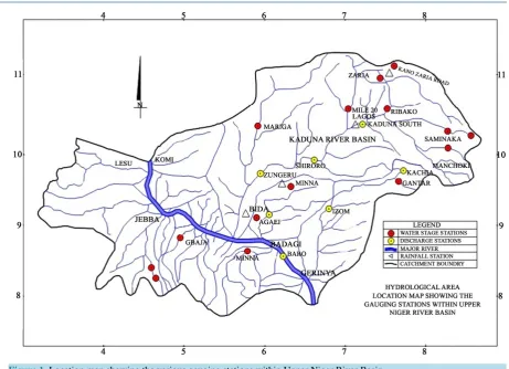
For this study, a total of 7 gauged sites (Kaduna, Shiroro, Kachia, Izom, Baro, Zungeru and Agaie) in the three selected rivers within the river basin controlling an area ranging from 900km2 to 6200 km2 were used. In this case, records of average monthly gauged flows for the respective rivers were obtained from Niger State and Kaduna State Water Boards as well as Power Holding Company of Nigeria (PHCN); these records were for gauging stations at Kachia and Izom (Gurara sub-basin), Kaduna, Shiroro and Zungeru (Kaduna sub-basin), and Agaie (Gbako sub-basin).Figure 1 shows the gauging stations whose records were employed for this study.

2.2. Study Protocol

The study is primarily patterned after some studies such as [7], [8], and [1], as well as [9]

Figure 1. Location map showing the various gauging stations within Upper Niger River Basin.

In the development of the FDC, catchment area was taken as the major characteristics in all the models; this choice was informed by the lack of available information on other catchment characteristics of interest. The FDCs were constructed by re-assembling the flow time series values in the decreasing order of magnitude as-signing flow values to class intervals and counting the number of occurrences (time steps) within each class in-tervals. Accumulated class frequencies were then calculated and expressed as a percentage of the total number of time steps in the record. The lower limit of every discharge class interval was plotted against the percentage points and then the discharges of exceedance percentage QP% (p = 1, 5, 10, …, 99) for each catchment were

cal-culated using specific FDC. Based on the submissions of [5], parametric method was employed in the regionali-sation protocol. In this approach, analytical functions were fitted to empirical flow duration curves in order to regionalise them. To do this, three basic probability distributions were considered; i.e., logarithmic, power and exponential.

Mathematical models of the flow duration curves were developed based on the logarithmic, power, and ex-ponential transformation framework. Resulting from this, the following equations were employed corresponding to the respective framework; that is, Equations (1)-(6)

( )

1 2ln

Q=a +a D (1)

2 1

b

Q=b D (2)

2

1e

c D

Q=c (3)

( )

1 2ln

Q

d d D

Q= + (4)

2 1

e Q

e D

2

1e

Df Q

f

Q= (6)

where, a–f are the coefficients, Q is the discharge; D is the Duration and Q is mean discharge.

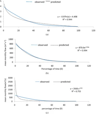
Figure 2 shows examples of the fitted plots for (i) logarithmic, (ii) exponential, and (iii) power models

By using regression analysis, the models as represented by Equations (1)-(3) and (4)-(6) were fitted to each set of paired values of Q versus D and Q Q versus D, respectively. The models with the Coefficient of Deter-mination (R2) closest to 1 were considered best fit with values of R2of Equations (1)-3), being statistically equal to that of Equations (4)-(6), respectively. Table 1 shows R2for the models for each station.

(a)

(b)

(c)

Figure 2. Examples of measured flow duration curves and the fitted lines from logarithmic, power and exponential models for Kaduna station.

Table 1.Regression coefficient or Coefficient of determination (R2) for the three models.

S/No. Location Logarithmic Equations (1)-(3) Power Equations (2) and (5) Exponential Equations (3) and (6)

1. Kaduna 0.94 0.75 0.99

2. Shiroro 0.96 0.76 0.96

3. Kachia 0.96 0.74 0.99

4. Izom 0.96 0.71 0.98

5. Baro 0.97 0.70 0.98

2) Regional Flow Duration Models

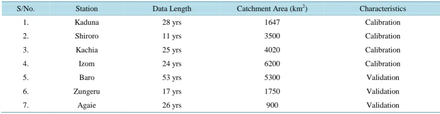
Three sub-basins of the Upper Niger River basin were selected for the study. These sub-basins, for the pur-poses of this study were (1) Kaduna, (2) Gbako, (3) and Gurara sub-basins. Details of stations (name, area and the period of the records) are as given in Table 2. The records for the seven stations were divided into two for the development of the FDC and regionalisation procedures. This split sampling approach required that some segments of the data were used for calibration and validation; to achieve this, five stations and the remaining two were used for calibration and validation, respectively.

Since the logarithmic and exponential models gave the highest values of average R2, model development was created from the data inTable 2 by establishing the relationship between drainage area and coefficients from the logarithmic and exponential models. The spatial variation coefficients were correlated with the drainage area.

Table 3shows the respective values of the coefficients a1, a2 and d1, d2 from the logarithmic models in

Equa-tions (1) and (4) and that of coefficients c1, c2 and f1, f2 from the exponential models in Equations (3) and (6),

respectively for each of the study locations. The plots for the determination of the regionalised parameters are as shown in Figures 3-6; these parameters so determined were then employed in the regionalisation framework.

Figure 3. Relationship between coefficients a1, a2 and drainage area at sub-basin level.

Figure 4. Relationship between coefficients c1, c2 and drainage area.

Table 2.Data segmentation for model development and simulation.

S/No. Station Data Length Catchment Area (km2_{) Characteristics}

1. Kaduna 28 yrs 1647 Calibration

2. Shiroro 11 yrs 3500 Calibration

3. Kachia 25 yrs 4020 Calibration

4. Izom 24 yrs 6200 Calibration

5. Baro 53 yrs 5300 Validation

6. Zungeru 17 yrs 1750 Validation

7. Agaie 26 yrs 900 Validation

y = 0.134x + 583.7 R² = 0.779

y = -3E-06x - 0.038 R² = 0.928

-200 0 200 400 600 800 1000 1200 1400 1600

0 1000 2000 3000 4000 5000 6000 7000

co

ef

fic

ien

t c

1

an

d c

2

Figure 5. Relationship between coefficients of d1, d2 and drainage area at sub-basin level.

Figure 6. Relationship between coefficients of f1, f2 and drainage area.

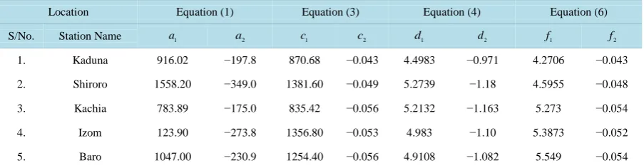
Table 3. Determined coefficient values for logarithmic and exponential models.

Location Equation (1) Equation (3) Equation (4) Equation (6)

S/No. Station Name a1 a2 c1 c2 d1 d2 f1 f2

1. Kaduna 916.02 −197.8 870.68 −0.043 4.4983 −0.971 4.2706 −0.043

2. Shiroro 1558.20 −349.0 1381.60 −0.049 5.2739 −1.18 4.5955 −0.048

3. Kachia 783.89 −175.0 835.42 −0.056 5.2132 −1.163 5.273 −0.054

4. Izom 123.90 −273.8 1356.80 −0.053 4.983 −1.10 5.3873 −0.052

5. Baro 1047.00 −230.9 1254.40 −0.056 4.9108 −1.082 5.549 −0.054

In doing so, the drainage area (A) and the coefficients were plotted to identify the relationships; The relation-ships were simply established by methods of least squares (i.e., Figure 1). The straight-line equations of the coefficients are as in Equations (7)-(14).

1 1 2

a = +j j A (7)

2 3 4

a = j + j A (8)

1 1 2

d = +k k A (9)

2 3 4

d =k +k A (10)

1 1 2

c = +l l A (11)

2 3 4

c = +l l A (12)

1 1 2

2 3 4

f =m +m A (14) The straight-line coefficients (j1 to j4, k1 to k4, l1 to l4 and m1 to m4) were further determined using regression

analysis. Table 4 shows the computed values for these coefficients.

The calculated basin values were inserted into Equations (7) and (8) for the dimensioned logarithmic and ex-ponential models and (12) to (13) for the dimensionless Logarithmic and exex-ponential models in order to com-pute the discharges (Q) corresponding to percent of time (D) at intervals increasing 1% each time up to 100%; for each station, these were computed and compared between the results from the Logarithmic and exponential models to find the best fitted model. Based on the re-parameterisation, Equations (15)-(18) were obtained; i.e., for the respective logarithmic and exponential schema.

(

) (

)

Q= j + j A + j + j A D (15)

(

)

(

(

)

( )

)

Q= I +I A I +I A D (16)

(

) (

) ( )

k k A k k D

Q= + + + (17)

(

)

(

(

)( )

)

Q

m m A m m A D

Q= + + (18)

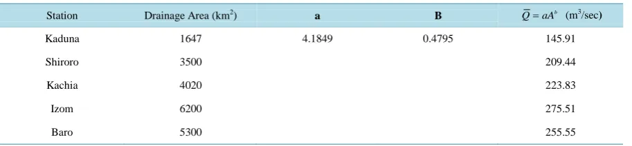
The estimation of each sub-basin’s representative average flow (Q) in Equations (20) and (21) was performed by analysing the relationship between mean annual flow and drainage area, as in Equation (19)

b

Q=aA (19)

where A is drainage area in km2; “a”as well as “b” are constants, their values are as presented in Table 5. Based on the re-parameterisation procedure, the regionalised models were obtained according as in Equations (20)- (21).

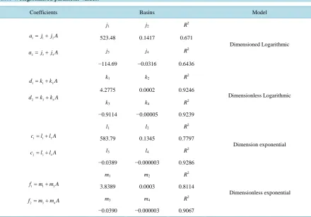
Table 4.Regionalised parameter values.

Coefficients Basins Model

1 1 2

a = +j j A

2 3 4

a =j +j A

j1 j2 R2

Dimensioned Logarithmic

523.48 0.1417 0.671

j3 j4 R2

−114.69 −0.0316 0.6436

1 1 2

d = +k k A

2 3 4

d =k +k A

k1 k2 R2

Dimensionless Logarithmic

4.2775 0.0002 0.9246

k3 k4 R2

−0.9114 −0.00005 0.9239

1 1 2

c = +l l A

2 3 4

c = +l l A

l1 l2 R2

Dimension exponential

583.79 0.1345 0.7797

l3 l4 R2

−0.0389 −0.000003 0.9286

1 1 2

f =m +m A

2 3 4

f =m +m A

m1 m2 R2

Dimensionless exponential

3.8389 0.0003 0.8114

m3 m4 R2

Table 5.Coefficients a, b and Q for each station.

Station Drainage Area (km2_{) a B} b

Q=aA (m3_/sec)

Kaduna 1647 4.1849 0.4795 145.91

Shiroro 3500 209.44

Kachia 4020 223.83

Izom 6200 275.51

Baro 5300 255.55

(

) (

) ( )

Q= I +I A + I +I A D ×aA (20)

(

)

(

(

)( )

)

b

Q= m +m A m + m A D ×aA (21)

where l1 to l4, m1 to m4, and a, b, are constants, respectively

3) Model Calibration and validation for flow prediction

To ascertain the adequacy or otherwise of the regional models, model calibration and validation were carried out. The accuracy of regional models was examined by using the measured discharges. In order to do this, measured and simulated results were compared in terms of root mean square relative error (ER)

(

)

100

1 100

100 2

1 m

c D

D R

Dm D

Q Q

E

Q

=

=

−

=

∑

∑

where D is the percent of time between 1% to 100%, QDcis the computed discharge at any percent of time; QDm

is the measured discharge at any percent of time. Using the coefficients J1 to J4, K1 to K4, l1 to l4 and m1 to m4,

the constants a, b and the drainage area of each station, the predicted discharges at 1% to 100% with interval 1% for each step or percentage of time (D) were determined from Equations (15)-(18).

3. Results and Discussion

3.1. Flow Variability and Issues of Consistency

Table 6shows the variability in the flow patterns for the stations considered; in this case, variability is on the

basis of low flow pattern. The low flow index though indicates that there may be some level of spatial correla-tion between the stacorrela-tions but whether this sparingly seeming correlacorrela-tion could provide for robust long-term pre-diction of flow in the ungauged stations becomes a matter of interest. This is imperative considering consistency related issues of the secondary data used for model calibration and validation since the prediction capability of the model is wholly depended on model conceptual assumptions and proper parameter estimation; in this context, the data length readily becomes a culprit. Because of the short length of data employed here, effective long-term generalisations may not really be practicable due to inherent vagaries. As noticed inTable 6, the high values of the low variation could be attributable to short falls in rainfall pattern coupled with problems of seasonality vis-à-vis climate change dynamics. In the overall, this could translate to long-term change in flow pattern; for this, the viable explanation for the foreseeable change pattern could be attributable to deleterious effects of an-thropogenic activities and variations in the hydroclimatology of the Basin writ large.

3.2. Performance of Regular and Regionalised FDCs

(a)

(b)

Figure 7. Simulated flow patterns for (a) Zungeru and (b) Agaie Station during the validation phase.

Table 6. Reliability and Streamflow variability.

S/No. Station

Low flow index

20

50

Q Q

50

90

Q Q

1. Kaduna 4.56 4.50

2. Shiroro 6.39 3.60

3. Kachia 6.60 7.14

4. Izom 4.80 10.00

5. Baro 4.20 14.29

6. Zungeru 1.41 1.73

7. Agaie 5.33 4.00

Table 7.Mean square relative errors (ER) in the calibration phase for logarithmic and exponential models.

ER of Model Validation

Station

FDC Model Dimensionless Model

Logarithmic, Equation (7) Exponential, Equation (8) Logarithmic, Equation (12) Exponential Equation (13)

Kaduna 25.43 8.81 31.45 27.74

Shiroro 36.75 17.95 35.15 31.58

Kachia 20.88 49.49 49.20 69.19

Izom 56.34 16.88 26.70 27.63

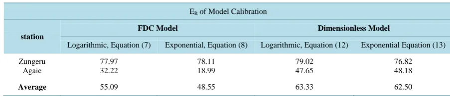
Baro 24.69 27.45 32.64 35.52

Table 8. Comparison of Root Mean Square Relative errors (ER) during verification for the logarithmic and exponential

mod-els.

ER of Model Calibration

station

FDC Model Dimensionless Model

Logarithmic, Equation (7) Exponential, Equation (8) Logarithmic, Equation (12) Exponential Equation (13)

Zungeru Agaie

77.97 32.22

78.11 18.99

79.02 47.65

76.82 48.18

Average 55.09 48.55 63.33 62.50

Table 9.Model forecast performance of extreme flow value for calibration stations.

S/No Station

Logarithmic Exponential

Rmax (%) Rmin (%) Rmax (%) Rmin (%)

1. Kaduna 95.81 65.8 95.57 52.65

2. Shiroro 70.31 56.7 76.41 79.30

3. Kachia 76.98 13.53 72.26 81.00

4. Izom 63.73 86.6 60.84 95.60

5. Baro 67.08 79.67 64.61 11.85

Average 74.0 60.0 73.0 64.00

Table 10. Model forecast performance in the validation phase.

S/No Station

Logarithm Exponential

Rmax (%) Rmin (%) Rmax (%) Rmin (%)

1. Zungeru 23.7 5.02 24.12 7.96

2. Agaie 73.98 6.95 76.83 11.47

Average 48.84 5.99 9.72 50.48

phases in terms of correlation metrics. It can be seen that the exponential model using FDC parameter gives reasonably well estimations of the FDC for the stations considered. However, in view of the short length of data used for the study, the model that gives the smallest root mean square relative error (ER) value can be used to

predict flow at the ungauged site within the Sub-basins. The contrasts between these values (ERand R2) should

not be related since ERis used to measure the prediction error of the proposed models whereas the values of R2

indicate how strong linear correlation existed between the model coefficients (i.e., a1, a2, e1, e2, f1, f2, j1, j2) and

the drainage area (A).

Despite the extent of correlation or relative error margins, it is pertinent to point that using just a representa-tive catchment characteristic may not be sufficient to reflect the hydrologic variation of a particular catchment as evidenced in Figure 7(a) where the model under predicted the entire flow regime even though it replicated the flow pattern. The high variability in the flow dynamics probably requires that the obvious need for the employ-ment of catchemploy-ment characteristics like slope and geology along with the drainage area parameter. This becomes essential especially considering how much overland flow vis-à-vis its time of concentration and the correspond-ing flow accumulation in streams/rivers and accretions are largely tied to catchment characteristics. In addition, using literally a threshold of 50% significant level of Rmax and Rmin[10] for high and low flows, respectively, the

4. Conclusion

Based on the findings of the study it is imperative to note that the regionalisation of flow duration curves is an effective approach for stream flow generation and extension, especially in the face of data scarcity. In addition, it is clearly evident that the use of catchment characteristics as input parameters, to a large extent for model de-velopment whether conceptual or statistical model in essential. However, results obtained by employing only the drainage area in the overall regionalised model indicate that it is not representative enough thus considering the length of data used and the attendant problem of flow variability, it suffices to note that an ensemble of catch-ment characteristics may be imperative. It is also important to take into consideration the ability of the models to reproduce the flow signatures; in this case, the prediction of extreme values is critical. Both the logarithmic and exponential function models employed in the FDCs portrayed different characteristics in the calibration and va-lidation stages. The exponentially regionalised models overwhelmingly performed better than the logarithmic as shown in the validation phase. Considering the results obtained in the overall, objective generalisations may not be possible though, the parameters obtained for the models in the regionalisation procedure were largely opti-mised. Hence, effective conclusion on the suitability of using the drainage area as a representative parameter in a copious attempt to understand the overall behaviour of a hydrologic response unit should be done with cautious optimism; especially taking cognisance of the implications of geologic characteristics of drainage basins in af-fecting low flows.

References

[1] Vogel, R.M. and Fennessey, N.M. (1994) Flow Duration Curves: New Interpretation and Confidence Intervals. Journal of Water Resources Planning and Management, 120, 485-504.

http://dx.doi.org/10.1061/(ASCE)0733-9496(1994)120:4(485)

[2] Smakhtin, V.Y. (2001) Low-Flow Hydrology: A Review. Journal of Hydrology, 240, 147-186.

http://dx.doi.org/10.1016/S0022-1694(00)00340-1

[3] Chiang, S.M., Tsay, T.K. and Nix, S.J. (2002) Hydrologic Regionalization of Watershed. II: Applications. Journal of Water Resources Planning and Management, 128, 12-20.

[4] Yu, P.S., Yang, T.C. and Wang, Y.C. (2002) Uncertainty Analysis of Regional Flow Duration Curves. Journal of Wa-ter Resources Planning and Management, 128, 424-430.

http://dx.doi.org/10.1061/(ASCE)0733-9496(2002)128:6(424)

[5] Castallarin, A., Galeati, G., Brandimarte, C., Montanari, A. and Brath, A. (2004) Regional Flow-Duration Curves Re-liability for Ungauged Basins. Advances in Water Resources, 27, 953-965.

http://dx.doi.org/10.1016/j.advwatres.2004.08.005

[6] Smakhtin, V.Y. and Watkins, D.A. (1997) Low-Flow Estimation in South Africa. Water Research Commission Report No. 494/1/97, Pretoria.

[7] Quimpo, R.G., Alejandrino, A.A. and McNally, T.A. (1983) Regionalised Flow Duration Curves for Philippines.

Journal of Water Resources Planning and Management, 109, 320-330.

http://dx.doi.org/10.1061/(ASCE)0733-9496(1983)109:4(320)

[8] Mimikou, M. and Kaemaki, S. (1985) Regionalisation of Flow Duration Characteristics. Journal of Hydrology, 82, 77- 91. http://dx.doi.org/10.1016/0022-1694(85)90048-4

[9] Rojanamon, P., Teweep, C. and Winyu, R. (2007) Regional Flow Duration Model for the Salawin River Basin of Thailand. ScienceAsia, 33,411-419.