Mathematical Modeling of Hydrogels Swelling Based on the Finite Element Method

Mathematical Modeling of Hydrogels Swelling Based on

the Finite Element Method

Armando Blanco1,2_{, Gema González}1_{, Euro Casanova}2_{, María E. Pirela}1,3_{, Alexander Briceño}3

1_{Centro de Ingeniería de Materiales y Nanotecnología, Instituto Venezolano de Investigaciones Científicas, Caracas, Venezuela} 2_{Departamento de Mecánica, Universidad Simón Bolívar, Caracas, Venezuela}

3_{Centro de Química, Instituto Venezolano de Investigaciones Científicas, Caracas, Venezuela}

Email: [email protected], [email protected], [email protected], [email protected], [email protected]

Received May 25, 2013; revised June 25, 2013; accepted July 5, 2013

Copyright © 2013 Armando Blanco etal. This is an open access article distributed under the Creative Commons Attribution License, which permits unrestricted use, distribution, and reproduction in any medium, provided the original work is properly cited.

ABSTRACT

In recent years, hydrogels have been introduced as new materials suitable for applications in areas such as biomedical engineering, agriculture, etc. The rate and degree of hydrogel swelling are important parameters that control the diffu- sion of drugs or solvents inside a polymer network. Therefore, the description of the dynamic swelling process of the hydrogels is very important in applications that require precise control of the absorption of solvents inside the hydrogel structure. To date, most of the numerical models developed for describing the swelling process are based in the finite difference methods. Even though numerical models supported in finite differences can be easily implemented, their use is limited to samples with very simple shapes. In this paper, a new model based on the finite element method is pro- posed. The diffusion equation is solved in a time-deformable grid. An original procedure is proposed to numerically solve the non-linear algebraic equation system that permits computing a new grid for each time-step. Hydrogel samples of different shapes were prepared in order to conduct experimental tests to validate the numerical proposed model. Nu- merical results show that the new model is able to describe the mass and shape changes in the hydrogel samples in time. An application of the numerical model to determine the relation between diffusion coefficients and density in Poly-acrylamide samples allows verifying the versatility of the model.

Keywords: Hydrogel Swelling; Diffusion Coefficients; Finite Elements

1. Introduction

Hydrogels are cross-linked polymeric networks that have the capability to hold water within their porous structure. This property allows using them in applications that re- quire either to absorb or to expel liquids from or towards the environment in which the hydrogel is immersed. Hy- drogel applications cover areas such as biomedical engi- neering, pharmaceutical industry, agriculture, etc. [1]. Some applications involve capturing or delivering liquids or mixtures in a dynamically controlled way, at predeter- mined rates for predefined periods of time. During the water uptake or delivery process, hydrogels could ex- perience volume changes of several orders of magnitude. According to Singh et al. [2], hydrogels can absorb amounts water nearly 10 - 20 times their molecular weight. Consequently, when a dry solid hydrogel sample is immersed in water, it suffers a continuous volume trans- formation until the ultimate, and completely swollen state is reached [1].

Depending on the application considered, dynamical description of the swelling process could be important. In some applications, only equilibrium hydrogel states need to be considered and the dynamic transient swelling proc- ess of the hydrogel does not need to be described [3-5].

However, some applications require prior knowledge of the transient behavior of the process of uptake or de-livery of drugs or solvents. For example, the description of the dynamic swelling process of the hydrogels is very important in applications that require precise control of the absorption of solvents inside the hydrogel structure.

Qualitative descriptions of the polymer relaxation pro- cess are reported by several authors [6,7]. Figure1 shows a diagram of the water sorption process into a hydrogel slab sample.

Figure 1. Qualitative description of polymer relaxation dur-ing water sorption into a slab geometry (adapted from [6]). White areas represent glassy polymer regions. Solvent ab-sorption corresponding to state (a) to (d) are detailed in the text.

rium concentration value). Therefore, water penetrates the dry polymer sample travelling from the hydrogel sur- face to its interior starting the hydrogel swelling process (Figure 1(a)). Thus, simultaneously, the surface of the hydrogel sample (swelling front) moves away from its core, while a mobile interface that separates dry and hy- drated polymer is displaced inside of the dry sample ( Fig-ure 1(b)). During this process, depending on the specific geometrical characteristic of the hydrogel sample, water concentration can reach its equilibrium value in the swell- ing front, or the dry-hydrated polymer interface disap- pears because water is present in all places of the hy- drogel sample (Figure 1(c)). Finally, water local concen- tration reaches its equilibrium value all around the hy- drogel sample (Figure 1(d)).

To describe the process of hydrogel volume change driven by water diffusion, different mathematical models have been developed. One approach is the so-called power-law equation where a simple empirical equation, developed by Peppas and Korsmeyer [8], assumes a time-dependent power law function which is used to de- termine the mechanism of diffusion in polymeric net- works

n t

M kt

M_  (1)

where Mt and M∞ are the cumulative amounts of water at time t and infinite time (equilibrium), respectively, k is a structural/geometric constant for a particular system and n is designated as “release exponent” representing the release mechanism [9].

Variations to the power-law function approach have been made in order to improve its capabilities to take into account some weaknesses. In particular, to take into ac- count both the solvent diffusion and the polymer relaxa- tion, Equation (1) was modified by Peppas and Sahlin [10]:

2

1 2

n t

M

k t k t M_  

n ₍₂₎

where k1, k2, and n are constants. Terms on the right side

represent the diffusion and polymer relaxation contribu- tion to the release profile, respectively.

Despite their simplicity, two drawbacks of the power- law function approach limit its use. First, it is necessary to determine the k’s and n coefficients, for each geomet- rical shape and size of the hydrogel sample. Second, no details of internal diffusion process such as position of the dry-hydrated polymer interface can be provided.

Another family of models have considered the combi- nation of the kinematics of the deformation, the presser- vation of solvent molecules, the local equilibrium condi- tions and the kinetics of the molecule migration, in order to simultaneously calculate the temporal evolution of the chemical potential of the solvent and the deformation of the hydrogel [11]. This approach can be implemented using a variational formulation, which leads to a set of coupled governing equations that describe mechanical and chemical equilibrium conditions, along with adequate boundary conditions [12,13]. The finite element method is frequently used to discretize the resulting system of differential partial Equations.

Even if such implementations enable numerical simu- lations of hydrogel swelling under various constraints, the later approach requires knowing or estimating a large number of physical parameters, such as, for example, values of the volume per solvent molecules, the envi- ronmental temperature, two dimensionless material pa- rameters to represent the Flory-Rehner free-energy den- sity function, besides of the coefficient of diffusion of the solvent in the hydrogel [11].

Between the two approaches described, a third class of models is found. In this approach, mathematical models based on Fick’s laws of diffusion [10] overcome limita- tions of the power-law Equation model and they do not require a very large number of parameters. In these mod- els, change in solvent concentration inside the hydrogel matrix are computed from [14]



C

_

D C t

 _{   }

 (3)

where C is the mass fraction of solvent in the hydrogel matrix, and D is the diffusivity. If the hydrogel deforma- tion due to osmotic stress is taken into account, Equation (3) can be modified to consider an elastic stress diffusion coefficient and the internal stress state of the polymer [9]. Nevertheless, for simple systems, authors as Rossi and Mazich [15,16] and Mazich et al. [17] have established that Fick’s law of diffusion is completely adequate to describe the swelling process.

ing process using Equation (3) needs to consider two different elements: the mathematical expression of the diffusivity coefficient and the volume change of the hy- drogel matrix during the swelling process. First, to de- scribe the diffusion process in the hydrogel matrix, the diffusivity coefficient cannot be considered constant. Good results [18,19] have been obtained by expressing the dif- fusion coefficients with a Fujita-type exponential de- pendence [20].

In addition, due to the intrinsic nature of the diffusion and penetration of the solvent in the matrix, the boundary between the hydrogel and the environment in which is immersed, the swelling front, moves during the swelling process (Figure 1). Consequently, the solution domain of the diffusion Equation (3) changes in time and a moving boundary condition needs to be included.

As a consequence of these last considerations, there are no analytical solutions to the mathematical model (3) with mobile boundary conditions, and these equations must be solved using a numerical method.

To date, most of the numerical models developed are based on the finite difference methods. Even though nu- merical models based on in finite differences can be eas- ily implemented, their use is limited to samples whose shape is very simple. Consequently, most applications are developed considering axial and radial diffusion within cylindrical tablets [18].

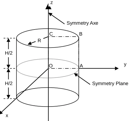
Figure2 shows the typical representation of the cylin- drical tablets and the symmetry plane and the symmetry axis, indicating the rectangular domain that represents the overall cylindrical tablet. The plane z = 0 cuts just in the top half of the tablet. The z-axis is a symmetry axis. Thus, a reduced computational domain, the rectangle OABC, can be used to model the solvent inflow into the

H/2

H/2

R

Symmetry Plane z

Symmetry Axe

y

x

O A B

C

Figure 2. Rectangular domain OABC representing overall cylindrical tablet for finite difference model.

cylindrical tablet. In the domain OABC, a rectangular grid can be generated. Therefore, the diffusion equation is easily discretized using a finite differences scheme.

During the swelling process, volume variations of the hydrogel sample are represented in a dynamically de- formable grid that is computed each time step. Mathe- matical models based on this approach have been suc- cessfully used in a vast range of applications [18,19]. Siepmann etal. [18] proposed a mathematical model for modeling the water transport into and drug release from hydroxypropyl methylcellulose (HPMC) cylindrical tab- lets. This model [18] considers that the tablet can swell in both axial and radial directions. The swelling is assumed to be ideal; the total volume of the tablet at any instant is given by the sum of the volumes of different components: polymer, water, and drugs. Thus, as the water penetrates the tablet, the total volume changes. In this manner, the tablet radius Rt and the half-height Ht change with time.

A rectangular grid is defined in the region = 0, 0 r Rt and 0 zHt. Once the new volume is computed in

each time interval, the new values of Rt and the Zt are

calculated. Due to that, [18] assumed that water imbibing in the axial direction leads to a volume increase in the axial direction, whereas water imbibing in the radial di- rection leads to a volume increase in the radial direction; the increase in volume in each direction is proportional to the surface area in this direction. In this approach, the shape of the tablet remains cylindrical during all the swelling process.

However, as it has been shown by Achilleos etal. [21], swelling is not a continual process [1]. Achilleos etal. [21] have developed a technique for the real-time visu-alization of dynamic deformation profiles during gel swelling processes. Achilleos et al. [21] visualizations allow appreciating that the evolution of the dry tablet shape does not necessarily preserve the initial cylindrical shape during all stages of the swelling process. When a hydrogel in its initial state is in contact with solvent molecules, the latter penetrate into the polymeric net- work. Obviously, the region close to the intersection be- tween the plane surface (z = Zt) and the cylindrical sur-

face (r = Rt) is exposed to a solvent flow on both surfaces.

Consequently, a more substantial increase in volume is expected in this region compared to the rest of the sur- face of the tablet.

On the other hand, the use of finite difference schemes in hydrogel samples different from cylindrical tablets can be restrictive because of the difficulties to generate a computational grid where diffusion equations can be eas- ily discretized. When non-rectangular grids are consid- ered, the interpolation process at the boundaries requires special considerations.

Finite element methods allow the use of adaptive grids non-restricted to rectangular elements. Therefore, non a priori restrictions to the sample shape during the swelling process need to be imposed. Additionally, initial sample shapes not limited to cylindrical tablets can be modeled. Even though the flexibility of the finite element method allows modeling arbitrary tridimensional sample shapes, for practical purposes, it is convenient, from a computa- tional point of view, to restrict sample shapes to bodies with a symmetry axis. Fortunately, this is the preferred shape in most practical applications. Figure3 shows typi- cal shapes that can be easily modeled with this approach.

In this study, the swelling dynamics of initially dry hydrogel samples is numerically modeled using the finite element method. Due to the numerical approach chosen, the sample shapes to be considered can correspond to those of any solid of revolution. The mathematical model is based on Fick’s second law of diffusion. The diffusion coefficient is expressed by a Fujita-type exponential de- pendence. The resulting equations are solved by using a deformable grid. Grid displacements are computed at the end of each time-step considering local variations in wa- ter concentration as a result of the diffusion process. The new positions of the grid nodes are computed by solving a set of non-linear equations that is solved for each time- step. This iterative process is done until the hydrogel sample reaches the final equilibrium state. Model valida- tion was performed by the comparison between numeri- cal results and laboratory tests, considering the swelling of hydrogel samples of different shapes (cylindrical tab- lets, conical and capsule samples).

This paper is organized in the following way. First, the mathematical model is presented. Equations for modeling the water diffusion process and sample shape evolution

(a) (b) (c) (d) (e)

Figure 3. Typical sample shapes and computational domain (in white) (a) cylindrical; (b) pastille; (c) capsule; (d) com-posed cone-cylinder and (e) general axisymmetry.

are developed. Then, a description of the numerical model, in particular, the specific implementation of the finite element model used to solve the diffusion equation and the finite difference scheme used to solve the grid equa- tions, is carried out. Later, the experimental section de- scribes the materials and methods used to prepare differ- ent hydrogel samples. Once the swelling laboratory tests for all hydrogel samples were finished, comparisons with numerical predictions were performed. Finally, following the analysis of results, model assumptions are evaluated and suggestions for further numerical and experimental work are provided.

2. Mathematical Model

In this study, the dynamics of the hydrogel swelling proc- ess is modeled. The following assumptions have been considered: 1) Dissolution processes are neglected, i.e., all solid material remains attached to the original sample; 2) Swelling can be modeled as a pure diffusion process; 3) Water concentration at the surface of the tablet is at its equilibrium value.

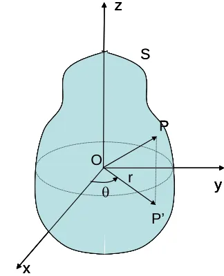
As a consequence of assumption 2) and following [18, 19], the mathematical model for modeling the water trans- port into the hydrogel samples is based on Fick’s second law of diffusion. A general sample and the cylindrical coordinate system are represented in Figure 4, just be- fore the swelling process starts.

Each point P in the hydrogel sample is represented by the coordinates r,  and z. The radial coordinate r, repre- sents the distance between the projected point of P, P’, in the plane xy and the origin O of the coordinate system; the axial coordinate, z, is the coordinate along the sym- metry axis and  is the angle between the segment OP’ and the x axis.

z

x

y r



P

P’ O

S z

x

y r



P

P’ O

z

x

y r



P

P’ z

x

y r



z

x

y r



P

P’ O

S

As there is no concentration gradient of any compo- nent with respect to , in cylindrical coordinates, Fick’s second law (3) is expressed as:

C C D C

D D

t r r r r z z

 _    _  _   

  

        

C

  (4)

where C and D are the concentration and the diffusion coefficient of water, respectively, r is the radial coordi- nate, z is the axial coordinate and t represents time.

To describe the diffusion process in the hydrogel ma- trix, the diffusivity coefficient is modeled following [18]. Thus, the diffusion coefficients is expressed with a Fu- jita-type [20] exponential dependence

exp 1 eq eq C D D C       _   _{ }

  (5)

where Deq and Ceq are the diffusion coefficient and sol-

vent concentration in the equilibrium swollen state of the system, respectively, and  is a dimensionless constant characterizing the concentration dependence of D.

The hydrogel sample is allowed to swell, independ- ently, in both axial and radial directions. The swelling is assumed to be ideal. Hence, the total volume of the sam- ple at any instant is given by the sum of the volumes of polymer and water. However, unlike the approach of [18], the hydrogel shape is not necessarily a cylindrical tablet. In particular, any form that corresponds to a solid of revolution can be modeled, as it is shown in Figure4.

At t = 0, the sample is dry and thus the water concen- tration at any position inside the sample is equal to zero while that at the sample surface, S, the water concentra- tion is Ceq. Thus, the initial conditions in each point P of

the hydrogel sample are expressed as: 0; 0 inside the sample 0; eq at the sample surface

t C P

t C C P

  

   (6)

During the swelling process, at the surface of the tablet, the concentration of water is assumed to be at its equilib- rium value, Ceq. This boundary condition is written as

follow:

0; _eq at the sample surface

t CC P (7)

During the swelling process, as a consequence of wa- ter inflow inside the hydrogel sample, the volume of the sample will change. Therefore, solution of the diffusion equation requires considering that the physical domain is changing along the swelling process. In addition, the sam- ple shape at each time is not known in advance and it is part of the solution.

3. Numerical Model

In this work, no assumption regarding the sample shape evolution was considered. In addition, because sample

shapes are not limited to cylindrical tablets, the selected numerical method should be able to manage irregular meshes. For these reasons, the finite element was chosen to discretize the mathematical model.

3.1. Finite Element Formulation

In order to obtain the finite element formulation of the problem, a weighted residual method, using the Galerkin formulation [22], was employed. The residual is defined from Equation (4) as:

 

R c D D

t r r r r z z

        

  _{ }  _ C_

          (8)

This residual is minimized by imposing:

 

Vol

R C v

 



where  is an arbitrary weight function that vanishes wherever a Dirichlet condition is specified, and dv = 2πrdA since the problem is axisymmetric.

Introducing (8) in (9) and manipulating the integrals, the weak formulation of the problem is obtained:

d d

d 0

A A

C C

r A D r A

t r r z z

C C r s r z       _   _                 _  _     







Using a Galerkin approach, the concentration and the weight function are interpolated from the nodal values by mean of the same matrix of interpolating functions:

 et e    Ψ C NC N (11)

With these interpolations, Equation (10) is transformed to:

     

T ₀

e e e e e e

t t t

e

   

 



where and are element matrices and vec- tors:

,

e e

M K f_{ }e_t

T _d e e A r A 

_

M N N (13)

T _d e e A D r 

_

K B B (14)

  T d

e e t C C r s r z       _  _    



f N (15)

where B represents the matrix of the derivatives of the interpolation function.

tion:

 t   t   



MC KC f_t



1

(16)

In this work, the finite element model was constructed using axisymmetric linear triangular elements of three nodes and one degree of freedom by node, corresponding to the concentration at that point.

3.2. Grid Generation

A grid made of triangular elements was generated in several steps for t = 0. Initially, the boundary profile of the symmetry plane of the hydrogel sample is repre- sented in the r-z plane (Step 0). Then, a first set of nr

segments was generated by building a number of straight lines between the origin of the coordinate system and the external boundary of the sample (Step 1). Thus, a second set of nz lines is generated. Each line of this second set

intersects those of the first set (Step 2). At this stage, the grid includes triangular and quadrilateral elements. Fi- nally, quadrilateral elements are divided to form triangu- lar elements (Step 4). Figure5 shows the different steps for the generation of the initial grid.

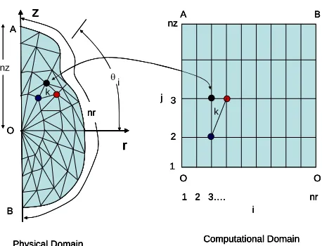
Figure6 shows the grid and the associated computa- tional domain.

A set of indices i and j, 1 inr and 1 jnz, repre-

sents each node (i, j) in the physical domain. Each node (i, j) has its representation in the computational domain. The origin in the physical domain is a “degenerated node”. It means that all nodes with j = 1 represent the origin O.

The total number of nodes is nrnz, whereas the total

number of elements is 2





Once the hydrogel sample starts the swelling process, the physical domain, and consequently, the computa- tional domain changes and a new mesh must be gener- ated each time-step. Then, it is necessary to establish nr

nz equations that allow computing the new position of

each node. The ensemble of equations is derived from: 1) Restricting the grid nodes to move along the nr original

lines (first set of lines); 2) symmetry condition along the z-axis and 3) volume of each element must contain the initial polymer mass and the water imbibed in.

z r Step 0 z r Step 0 z r Step 1 z r Step 1 z r Step 2 z r Step 2 z r Step 3 z r Step 3

Figure 5. Generation process for the initial grid.

z r z r O A B O O A B nr nz

1 2 3…. nr 1

2 3 nz

v

Physical Domain Computational Domain

i j k k _i z r z r O A B O O A B nr nz

1 2 3…. nr 1

2 3 nz

v

Physical Domain Computational Domain

i j k k z r z r O A B O O A B nr nz

1 2 3…. nr 1

2 3 nz

v

Physical Domain Computational Domain

i j

k

k

_i

Figure 6. k-element in the physical and computational do-main.

Condition 1) requires that, if i is the angle between

the i-line and the r-axis, then

1,

,

0 1 tan 1 ; 1 0 1

j

ij ij i

nr j

r j nr

z r i nr j n

r j nr

    r         (17)

The symmetry condition 2) imposes that grid lines are orthogonal to the z-axis. Thus,

0 0 r z r _  _

 (18)

The resulting algebraic equation set from expression (18) can be expressed by using a forward or backward second order expression in finite differences. For exam- ple, for i=1, using forward finite differences







2 2

3 2 2 3

1

2 3 2 3

2

j j j j

j

j j j j

z r z r

z j

r r r r



nz

  

  (19)

Finally, condition 3) needs to consider spatial local variation of water in each elementary grid element in time. In consequence, equations that express the relation between local water concentration and the volume of each element must be established.

The strategy to generate the new grid considers that the local mass of each mesh elementary volume at time t, mk, is given by

 

k k k

m mp mw t (20) where mpk and mwk are the polymer mass and water mass

at element k. The mass mpk is constant and it corresponds

to the original mass of dry polymer at t = 0 at element k. In terms of the local water concentration, the mass in the k-element can be expressed as

 



 



   

k p k w k k

where p and w are the polymer and water volumetric

density, respectively, Vk(t) and Ck(t) are the total volume

and the water concentration in the k-element.

A expression such as Equation (21) can be written at t = t + t















 



k

p k w k k

m t t

C t t C t t V t t

 

 

 

_       _   (22)

Because the polymer mass is constant in the k-element, the first term on the right side of Equations (21) and (22) are equal and















 



 

        (23)

Taking advantage of the geometrical properties of the hydrogel sample, the elementary volume for a solid of revolution is calculated from:

 

   

k k k

V t  r t A t (24) where rk(t) and Ak(t) are the centroid position and the

area of the triangle associated to the k-element at the in- stant t.

With (24) in (23) after some simplifications it gives



 



_

 

_{    }

1

k

k k k k

k

C t

A t t r t t A t r t

C t t



    

   (25)

The non-linear Equations (17), (19) and (25) are a complete set of algebraic equations that permits generat- ing a new mesh each time-step.

However, when all non-linear nr nz algebraic equa-

tions are solved simultaneously, some convergence prob- lems were found. In order to avoid these problems, a numerical solution solving layer by layer was imple- mented. In this approach, the origin coordinates (corre- sponding to j = 1) are constant. The implemented proce- dure starts by finding the position of the grid nodes cor- responding to j = 2 for t = t + t. Hence, only nr non-

linear algebraic equations must be solved. Once these nodes coordinates are found, the next level, j = 3, is solved. This procedure continues until the node coordi- nates corresponding to the level j = nz are found. In this

way, a set of nr non-linear algebraic equations are solved nz times instead of a single nznr system. This procedure

converged in all simulated cases.

An additional simplification, with high impact on com- putational time, can be introduced when the physical domain has a symmetry plane, as in the case of a cylin- drical tablet. In such cases, a symmetry condition as Equa- tion (18) can be implemented. Then, if the symmetry plane corresponds to z = 0, the symmetry condition will be

0

0

z

r z _

 

 (26)

4. Materials and Methods

To validate the numerical model, a number of laboratory tests were conducted considering different sample shapes such as cylindrical tablets, capsules, pastilles and com- posed cone-cylinder (Figure 3). The hydrogel samples were prepared using the following materials and meth- ods.

4.1. Materials

The following compounds were obtained from Sigma Aldrich: Acrylamide (AAm, +99% purity), N’N’metile- nebisacrylamide (NMBAAm, +99% purity) and Ammo- nium Persulfate (PSA, +98% purity).

4.2. Methods

Polyacrylamide hydrogel was synthesized by chemical initiation, using AAm (1 g) as monomer, and N’N’Me- thylenebisacrylamide (11 mg) as crosslinking agent; these were mixed in 0.7 ml of distilled water for 5 min-utes; then PSA was added as initiator of the reaction. The synthesis was carried out in a thermal bath, at a tempera- ture of 30˚C ± 1˚C, under constant stirring of 200 rpm. The resultant monolith was cut in discs of different lengths. The measurements of absorption were obtained introducing the dry hydrogel discs (previously weighed, mo) in distilled water at 37˚C. The swollen hydrogels, for

predetermined times (up to equilibrium swelling), were removed and gently dried with a filter paper to remove excess water and finally weighed (mt) in a scale (Adven-

ture-OAUS with an accuracy of ±0.0001 g). The swelling percentage (%S) of the hydrogels was determined from the following relation:

0

0

100

t

m m S

m



 (27)

During the swelling process, special care was taken to assure that the hydrogel sample was fully immersed in the distilled water avoiding contact with the walls of the recipient.

5. Numerical Results

Applications of the numerical model require advanced knowledge of three unknown parameters: the diffusion coefficient Deq, the dimensionless constant , and the

solvent concentration in the equilibrium swollen state of the system, Ceq.

The constant  is characteristic of the diffusing mole-cules and, for water, a value of 2.5 was calculated by Siepmann etal. [18]. The diffusion coefficient of water Deq within the fully swollen hydrogel must be determined

Ceq, depends on the particular capability of the xerogel to

absorb water and is determined for measuring the total amount of water in fully swollen hydrogel samples.

Since the main objective of this work is to develop a numerical method that considers the actual shape evolu- tion of the hydrogel sample during the solvent absorption process using few parameters, the diffusion coefficient of water Deq was computed by numerical regression in order

to fit the experimental data. Consequently, influence of variations in Deq due to changes in experimental condi-

tions (size of recipient, position of the hydrogel particular sample in the original bulk, etc.) was not considered.

To validate the capabilities of the numerical model, three different kinds of samples were considered: 1) tab- lets; 2) capsules and 3) truncated cones.

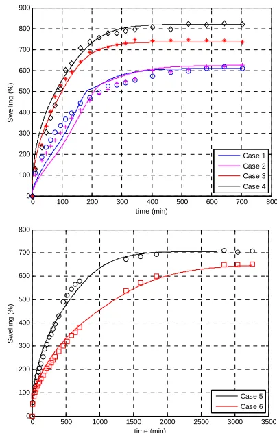
Six different cylindrical tablets were considered. The particular characteristic of each sample are reported in

Table 1.

Figure 7 shows the transient water uptake for each cy- lindrical tablet.

The match between experimental data and numerical model predictions is remarkable. In all analyzed cases, the proposed model was able to reproduce the dynamic water uptake.

A typical sample shape evolution and water penetra- tion is shown in Figure 8. Initially, water uptake is more pronounced in the intersection of the top and bottom of the sample and the cylindrical wall. Consequently, this region swells more than the other surfaces of the sample.

This trend is in good agreement with experimentally observed behaviour, as shown in Figure9.

Qualitatively, it is clear from Figure9 that numerical predictions of shape evolution in time correspond to ex- perimental behaviour.

Other sample with shape corresponding to a truncated cone was modelled. Figure10 shows the initial shape of the truncated cone. This kind of sample shape cannot be modelled using the classical finite difference models.

Figure 11 shows the water uptake process for the trun- cated cone. The finite element model was able to repro- duce accurately the swelling process.

Table 1. Geometrical and physical properties of cylindrical tablet samples.

Sample Radius (mm) Thickness (mm) Mass (gr) Density (gr/cm3₎

1 2.1377 2.7955 0.0324 0.8073

2 2.8831 2.4467 0.0558 0.8733

3 4.1899 2.1419 0.0832 0.7043

4 4.7729 7.2110 0.2709 0.5249

5 4.8842 8.9300 0.4997 0.7466

6 4.7958 8.7904 0.5649 0.8893

Finally, the finite element model was applied to ana- lyze the relation between diffusivity coefficients and sam- ple average density. Figure 12 shows the variations be-

0 100 200 300 400 500 600 700 800

0 100 200 300 400 500 600 700 800 900

time (min)

S

w

el

ling (

%

)

Case 1 Case 2 Case 3 Case 4

0 500 1000 1500 2000 2500 3000 3500

0 100 200 300 400 500 600 700 800

time (min)

S

w

el

li

ng

(%

)

Case 5 Case 6

Figure 7. Fit of the model to water uptake. Experimental Data(markers)-Numerical model (lines). Sample details in Table 1.

(a) (b)

(c) (d)

Figure 9. Typical shape evolution in a circular tablet (a) t = 5 min; (b) t = 15 min; (c) t = 35 min and (d) t = 72 h.

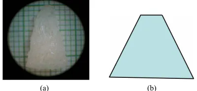
(a) (b)

Figure 10. Truncated cone: (a) Physical sample; (b) Physi-cal domain.

0 100 200 300 400 500 600 700

0 40 80 120 160 200 600

400

200

0

time (min) S (%)

0 100 200 300 400 500 600 700

0 40 80 120 160 200 600

400

200

0

time (min) S (%)

Figure 11. Fit of the model to water uptake in non-cylin- drical sample shapes: Truncated cone.

Figure 12. Relation between density and diffusion coeffi-cients.

tween both properties.

From the inspection of Figure 12, it is clear that the diffusion coefficient diminish with sample density. The reasons for this behavior will be the subject of attention of future work.

6. Conclusions

This work presents a numerical model, based on the fi- nite element method that describes the swelling process in hydrogel samples. The diffusion equation was solved in a time-deformable grid. The diffusion coefficients were expressed by a Fujita-type exponential dependence. An original procedure that considered local variations in wa- ter concentration to displace the nodes of the grid was implemented.

The model performance was tested by comparing nu- merical swelling predictions with laboratory experimen- tal measures obtained from Polyacrylamide hydrogel sam- ples of different shapes, such as cylindrical tablets and truncated capsules and cones.

Numerical results show that the new model is able to describe the mass and shape changes in the hydrogel sample in time using very few parameters. Even though the initial and final shapes of the hydrogel samples are the same, the shape of the hydrogel sample dramatically changes during the swelling process.

Qualitative comparisons with experimental tests show that the new numerical model is able to predict the dy-namic shape of the hydrogel sample. Versatility of the model was verified through the determination of the rela- tion between diffusion coefficients and densities for an ensemble of Polyacrylamide samples.

The proposed model does not take into account the elastic effects due to the change in polymer structure. This aspect will be included in a future work.

REFERENCES

[1] F. Ganji, S. Vasheghani-Farahani E. and Vasheghani-Fa- rahani, “Theoretical Description of Hydrogel Swelling: A Review,” Iranian Polymer Journal, Vol. 19, No. 5, 2010, pp. 375-398.

[2] A. Singh, P. K. Sharma, V. K. Garg and G. Garg, “Hy- drogels: A Review,” International Journal of Pharma- ceutical Sciences Review and Research, Vol. 4, No. 2, 2010, pp. 97-105.

[3] T. L. Porter, R. Stewart, J. Reed and K. Morton, “Models of Hydrogel Swelling with Applications to Hydration Sensing,” Sensors, Vol. 7, No. 9, 2007, pp. 1980-1991. doi:10.3390/s7091980

[4] P. J. Flory and J. Rehner, “Statistical Mechanics of Cross- Linked Polymer Networks I,” Journal of Chemical Phys-ics, Vol. 11, No. 11, 1943, pp. 512-520.

doi:10.1063/1.1723791

Linked Polymer Networks II,” Journal of Chemical Phy- sics, Vol. 11, No. 11, 1943, pp. 521-526.

doi:10.1063/1.1723792

[6] C. S. Brazel and N. A. Peppas, “Dimensionless Analysis of Swelling of Hydrophilic Glassy Polymers with Subse- quent Drug Release from Relaxing Structures,” Biomate-rials, Vol. 20, No. 8, 1999, pp. 721-732.

doi:10.1016/S0142-9612(98)00215-4

[7] P. A. Sandoval, Y. Baena, M. Aragón, J. Rosas and L. Ponce, “Overall Mechanisms That Rule the Active Phar- maceutical Ingredient’s Delivery Process from Hydro- philic Matrices Elaborated with Ether Cellulose,” Revista Colombiana de Ciencias Químico-Farmacéuticas, Vol. 37, No. 2, 2008, pp. 105-121.

[8] N. A. Peppas and R. W. Korsmeyer, “Dynamically Swell- ing Hydrogels in Controlled Release Applications,” In: N. A. Peppas, Ed., Hydrogels in Medicine and Pharmacy, CRC Press, Boca Raton, 1987.

[9] D. De Kee, Q. Liu and J. Hinestroza, “Viscoelastic (Non- Fickian) Diffusion,” The Canadian Journal of Chemical Engineering, Vol. 83, No. 6, 2005, pp. 913-929.

doi:10.1002/cjce.5450830601

[10] N. A. Peppas and J. J. Sahlin, “A Simple Equation for the Description of Solute Release. III. Coupling of Diffusion and Relaxation,” International Journal of Pharmaceutics, Vol. 57, No. 2, 1989, pp. 169-172.

doi:10.1016/0378-5173(89)90306-2

[11] J. Zhang, X. Zhao, Z. Suo and H. Jiang, “A Finite Ele-ment Method for Transient Analysis of Concurrent Large Deformation and Mass Transport in Gels,” Journal of Applied Physics, Vol. 105, 2009, Article ID: 092532. [12] M. Kang and R. Huang, “A Variational Approach and

Finite Element Implementation for Swelling of Polymeric Hydrogels under Geometric Constraints,” Journal of Ap- plied Mechanics, Vol. 77, 2010, Article ID: 061004, 12 Pages.

[13] W. Hong, X. Zhao, J. Zhou and Z. Suo, “A Theory of Coupled Diffusion and Large Deformation in Polymeric Gels,” Journal of the Mechanics and Physics of Solids,

Vol. 56, No. 5, 2008, pp. 1779-1793 doi:10.1016/j.jmps.2007.11.010

[14] J. Crank, “The Mathematic of Diffusion,” 2nd Edition, Clarendon Press, Oxford, 1979.

[15] G. Rossi and K. A. Mazich, “Kinetics of Swelling for a Cross-Linked Elastomer or a Gel in the Presence of a Good Solvent,” Physical Review A, Vol. 44, No. 8, 1991, pp. R4793-R4796. doi:10.1103/PhysRevA.44.R4793 [16] G. Rossi and K. A. Mazich, “Macroscopic Description of

the Kinetics of Swelling for a Cross-Linked Elastomer or a Gel,” Physical Review E, Vol. 48, No. 2, 1993, pp. 1182-1191. doi:10.1103/PhysRevE.48.1182

[17] K. A. Mazich, G. Rossi and C. A. Smith, “Kinetics of So- lvent Diffusion and Swelling in a Model Elastomeric System,” Macromolecules, Vol. 25, No. 25, 1992, pp. 6929-6933. doi:10.1021/ma00051a032

[18] J. Siepmann, K. Podual, M. Sriwongjanya, N. A. Peppas and R. Bodmeier, “A New Model describing the Swelling and Drug Release Kinetics from Hydroxypropyl Methyl- cellulose Tablets,” Journal of Pharmaceutical Sciences, Vol. 88, No. 1, 1999, pp. 65-72.

doi:10.1021/js9802291

[19] J. Siepmann, H. Kranz, R. Bodmeier and N. A. Peppas, “HPMC Matrices for Controlled Drug Delivery: A New Model Combining Diffusion, Swelling and Dissolution Mechanisms and Predicting the Release Kinetics,” Phar- maceutical Research, Vol. 16, No. 11, 1999, pp. 1748- 1756. doi:10.1023/A:1018914301328

[20] H. Fujita, “Diffusion in Polymer-Diluent Systems,” For- tschritte Der Hochpolymeren-Forschung, Advances in Polymer Science, Vol. 3, No. 1, 1961, pp. 1-47.

[21] E. C. Achilleos, R. K. Prudhomme, K. N. Christodoulou, K. R. Gee and I. G. Kevrekidis, “Dynamic Deformation Visualization in Swelling of Polymer Gels,” Chemical Engineering Science, Vol. 55, No. 17, 2000, pp. 3335- 3340. doi:10.1016/S0009-2509(00)00002-6