a s p h e r e wi t h n o nli n e a r
Bo u s si n e s q a p p r o xi m a ti o n
Vas u , B, Go rl a , R S R, B e g , OA, M u r t hy, PV SN, P r a s a d , VR a n d K a dir,
A
h t t p :// dx. d oi.o r g / 1 0 . 2 5 1 4 / 1 .T 5 5 1 6
T i t l e U n s t e a d y flo w of a n a n ofl ui d ov e r a s p h e r e wi t h n o n li n e a r Bo u s si n e s q a p p r o xi m a ti o n
A u t h o r s Vas u , B, Go rl a, R S R, B e g , OA, M u r t hy, PV SN, P r a s a d , VR a n d Ka dir, A
Typ e Ar ticl e
U RL T hi s v e r si o n is a v ail a bl e a t :
h t t p :// u sir. s alfo r d . a c . u k /i d/ e p ri n t/ 4 7 8 6 1 /
P u b l i s h e d D a t e 2 0 1 8
U S IR is a d i gi t al c oll e c ti o n of t h e r e s e a r c h o u t p u t of t h e U n iv e r si ty of S alfo r d . W h e r e c o p y ri g h t p e r m i t s , f ull t e x t m a t e r i al h el d i n t h e r e p o si t o r y is m a d e f r e ely a v ail a bl e o nli n e a n d c a n b e r e a d , d o w nl o a d e d a n d c o pi e d fo r n o
n-c o m m e r n-ci al p r iv a t e s t u d y o r r e s e a r n-c h p u r p o s e s . Pl e a s e n-c h e n-c k t h e m a n u s n-c ri p t fo r a n y f u r t h e r c o p y ri g h t r e s t r i c ti o n s .
AIAA JOURNAL OF THERMOPHYSICS AND HEAT TRANSFER
AIAA PUBLISHING, VIRGINIA, USA.ISSN: 0887-8722; EISSN: 1533-6808; Impact Factor: 1.315 Accepted July 15th 2018
UNSTEADY FLOW OF A NANOFLUID OVER A SPHERE
WITH NON-LINEAR BOUSSINESQ APPROXIMATION
B. Vasu1, Rama S. R. Gorla2*, O. Anwar Bég3, P. V. S. N. Murthy4 , V. R. Prasad5 and A. Kadir 3
1Department of Mathematics, Motilal Nehru National Institute of Technology, Allahabad - 211004, India. 2Department of Mechanical Engineering, Cleveland State University, Ohio, USA.
3Department of Mechanical and Aeronautical Engineering, Salford University, Salford, M54WT, UK. 4Department of Mathematics, Indian Institute of Technology Kharagpur, Kharagpur, India.
5Department of Mathematics, Madanapalle Institute of Technology and Science, Madanapalle-517325, India. Abstract:A theoretical study is presented of transient mixed convection boundary layer flow of a nanofluid in the forward stagnation region of a heated sphere which is rotating with time dependent angular velocity. The effect of the non-linear Boussinesq approximation is taken into account. The nanofluid is treated as a two-component mixture i.e. nano-particles distributed homogenously in a base fluid (water or gas). The effects of the Brownian motion and thermophoresis are included for the nanofluid and constant wall temperature is imposed at the sphere surface. The first and second laws of thermodynamics are employed in order to study thermophysics as well as heat and mass transfer phenomena. By introducing appropriate similarity variables the governing equations are transformed into a system of dimensionless, nonlinear, coupled, ordinary differential equations which are solved numerically by applying the second-order accurate implicit finite difference Keller box method. The reliability and efficiency of the obtained numerical results are validated via comparison with the previously published results for special cases. The effects of various parameters on primary and secondary velocities, temperature, nanofluid volume fraction (concentration), primary and secondary shear stress functions, Nusselt number function (wall heat transfer rate) and Sherwood number function (wall nano-particle mass transfer rate) are visualized. Furthermore the influence of non-linear temperature parameter, Brinkman parameter (ratio of Brinkman number to dimensionless temperature ratio), local Reynolds number and unsteadiness parameter on entropy generation number is computed. A strong elevation in entropy generation number is computed with both increasing Brinkman parameter and unsteadiness parameter. Primary and secondary surface shear stresses, Nusselt number and Sherwood number also increase with unsteadiness and rotation parameters. Primary shear stress is boosted with increasing mixed convection parameter and Brownian motion effect whereas secondary shear stress is depressed. Temperatures are suppressed with increasing nonlinear temperature parameter whereas nano-particle concentrations are elevated. Increasing thermophoresis parameter enhances both temperatures and nano-particle concentration values. The simulations find applications in rotating chemical engineering mixing systems and nano-coating transport phenomena.
Keywords: Non-linear mixed convection; stagnation flow; nanofluids; Brownian motion; Keller-box method; entropy generation; Brinkman number; unsteadiness; rotation.
NOMENCLATURE
A unsteadiness parameter C concentration
Cfx friction factor
DB Brownian diffusion coefficient [m-2 s-1]
DT thermophoretic diffusion coefficient [m-2 s-1]
f dimensionless stream function
k effective thermal conductivity [W m-1 K-1] Nb Brownian motion parameter
Br Brinkman number,
2 e
u k T
Nt thermophoresis parameter Nu Nusselt number
Pr Prandtl number Grx local Grashof number
Rex local Reynolds number
Sc Schmidt number T temperature [K]
TW wall temperature of the vertical plate [K]
𝑇∞ ambient temperature [K]
x, y coordinates along the plate generator and normal to the generator respectively u, v velocity components along the x- and y- directions respectively
t time
t dimensionless time
Ng dimensionless entropy generation number
Greek Symbols:
αm thermal diffusivity of porous medium [m-2 s-1]
1
non-linear temperature (related to nonlinear Boussinesq approximation)
𝜂 dimensionless transverse coordinate θ dimensionless temperature
μ viscosity of fluid [kg m-1 s-1] λ dimensionless rotation parameter λ1 mixed convection parameter
ρf fluid density [kg m-3]
ρp nano-particle mass density [kg m-3]
(ρc)f heat capacity of the fluid [J m-3 K-1]
(ρc)m effective heat capacity of porous medium [J m-3 K-1]
(ρc)p effective heat capacity of nano-particle material [J m-3 K-1]
dimensionless nano-particle volume fraction ψ stream function
1. INTRODUCTION
Convective heat transfer is significant in numerous industrial heating or cooling devices. Heat convection can be modified by altering flow geometry, boundary conditions or by enhancing fluid thermophysical properties. A popular methodology for achieving this which has emerged in recent years is via doping of the working fluids in thermal engineering systems with very small solid particles. Fabricating particles at the nanoscale and selective suspension in base fluids creates solid–liquid mixtures known as nanofluids. Nanofluids therefore constitute a new kind of heat transfer fluid containing small quantities of nano-sized particles (usually less than 100 nm) which are uniformly and stably suspended in a liquid. The dispersion of a small amount of solid nanoparticles in conventional fluids changes their thermal conductivity remarkably. The term “nanofluid” was introduced by Choi [1] who initiated the synthesis of colloidal suspensions of nanoparticles in the base fluids. These fluids represent an innovative way to increase thermal conductivity and, therefore, heat transfer performance of industrial systems. Unlike heat transfer in conventional fluids, the exceptionally high thermal conductivity of nanofluids manifests in enhanced heat transfer rates, a unique feature of nanofluids. Nanofluid behaviors have been observed consistently by different many researchers and various metallic nanoparticles have been explored including copper, titanium oxide and silver owing to the high thermal conductivity of these metals. Various base fluids include ethylene glycol, water, oils, air etc. An early theoretical model for nanofluid transport phenomena was proposed by Buongiorno [2]. Zau Wu et al. [3] experimentally investigated the pressure drop and heat transfer characteristics of alumina/water nanofluids in helical heat exchangers. Ulzie Rea et al. [4] studied experimentally the laminar convective heat transfer and viscous pressure loss for alumina–water and zirconia–water nanofluids in a flow loop with a vertical heated tube, noting that the heat transfer coefficient enhancement is strongly related to the different mixture properties of the nanofluids. Several authors have attempted to develop convective transport for nanofluids as homogeneous flow models. Das et al. [5] presented a popular model which incorporates volume fraction via modified nanofluid thermophysical properties in the momentum and energy equations, but does not include a species conservation equation as featured in the Buongiorno model (this model emphasizes Brownian motion and thermophoresis effects). Kuznetsov and Nield [6] described recent experimental and theoretical studies on convective heat transfer in nanofluids and further identified some challenges and opportunities for future research. Gorla and Hossain [7] simulated mixed convective boundary layer flow over a vertical cylinder embedded in a porous medium saturated with nanofluid. Kameswaran et al. [8] studied numerically the convective heat transfer in non-Darcy nanofluid flow over a vertical wavy surface incorporating the influence of non-linear Boussinesq approximation, thermal stratification and convective boundary conditions. Srinivasacharya and Surender [9] evaluated the effect of double stratification on mixed convection flow of a nanofluid along a vertical plate embedded in non-Darcy porous medium. Bég et al. [10] investigated with MAPLE numerical quadrature the hydrodynamic, thermal and mass slip effects in transient asymmetric bioconvective nanofluid flow in a porous microchannel with deformable walls. The influence of viscous dissipation and chemical reaction on convective transport in a boundary layer stagnation point nanofluid flow from a stretching/shrinking sheet has been considered by Murthy et al. [11]. Recently, Gorla and Vasu [12] studied unsteady convective heat transfer to a stretching surface in a non-Newtonian nanofluid.
turbines, thermal plasma processing and paint spray mechanisms. Takhar and Nath [13] have reported a self-similar solution for transient stagnation-point boundary layer flow from a rotating sphere with magnetic field effects. Anilkumar and Roy [14] investigated unsteady mixed convection boundary layer flow in the stagnation point region of a rotating sphere where the free stream velocity and angular velocity of the rotating sphere vary continuously with time. Bég et al.
[15] studied the nonlinear magnetized thermal convection from a rotating cone in anisotropic porous media using a finite difference method. Chamkha and Ahmed [16] have presented numerical finite difference solutions for unsteady magnetohydrodynamic mixed convection heat and mass transfer from a rotating sphere. Bég et al. [17] used an optimized homotopy analysis method (HAM) to study stagnation-point nanofluid flow from a spinning sphere, verifying the sensitivity of boundary layer characteristics to rotational and unsteady effects. Thumma et al. [18] presented variational finite element solutions for unsteady dissipative hydromagnetic convective heat and mass transfer in nanofluid flow from a rotating perforated plate in porous media.
The study of nonlinear heat convection has substantial relevance in both engineering and geo/astro-physical flows. In the conventional Boussinesq approximation, density differences are sufficiently small to be neglected, except where they appear in terms multiplied by gravity and the convention is to use a single linear thermal buoyancy term in the momentum equation. This restricts the application of models to lower temperature differences. In the non-Boussinesq approximation a temperature-concentration-dependent density relation is employed and this also allows non-linear temperature variation. Non-Boussinesq flows have been studied in several different areas of thermal sciences. Kamel and Paolucci [19] simulated using the FIDAP finite element code, the thermofluid transport in a furnace for fabricating carbon aircraft brakes, noting that a more robust simulation is possible for a wider variation of properties with temperature with a non-Boussinesq model. Van der Borght [20] studied nonlinear convection numerically in a compressible medium of polytropic structure using a band matrix algorithm and considering two characteristic density stratifications. Partha [21] reported on the effects of nonlinear convection with nonlinear temperature and concentration in a porous medium using the non-Boussinesq temperature-concentration-dependent density relation. Sameen et al. [22] studied non-Boussinesq convection in low temperature gaseous helium at intermediate Rayleigh numbers, observing that the Nusselt number is reduced as the system departs from the Boussinesq approximation. Hung and Cheng [23] investigated computationally the free convection of non-Boussinesq fluid in a rectangular enclosure, showing that better accuracy is achieved for high temperature differences compared with the conventional Boussinesq approximation.
.
suppressed with thermal radiation whereas it is elevated with viscous dissipation (fluid friction). Chen and Liu [28] studied the entropy generation in magneto-hydrodynamic mixed convection flow of nanofluid within a vertical asymmetrically-heated parallel-plate channel subjected to viscous dissipation effect. Adesanya et al. [29] considered entropy generation in third grade Reiner-Rivlin viscoelastic fluid convection. Gorla et al. [30] used a power-law model to study entropy generation in thermal convection boundary layer flow from a two-dimensional wedge to a non-Newtonian saturated porous medium, observing that Bejan number is enhanced with both viscosity index (non-Newtonian parameter) and the buoyancy parameter.
The aim of the present work is to study the entropy analysis on mixed convective boundary layer flow of nanofluid at the stagnation point region of a rotating sphere. Non-linear convection is examined with a second-order approximation of temperature (non-Boussinesq approximation). The sphere surface is assumed to be isothermal (constant wall temperature). In the following sections, the problem is formulated, analyzed, solved numerically with a finite difference code with validation also included. An entropy generation analysis is also performed. Both gaseous and water base fluids are considered. Buongornio’s model [2] is utilized for nanoscale effects. The influence of the emerging thermo-physical parameters on fluid, heat and mass transfer characteristics are determined and illustrated graphically. The computations are relevant to nano-coating spin processing in the chemical engineering industry.
2. MATHEMATICAL MODEL
Consider an unsteady mixed convection boundary layer flow in the forward stagnation point region of heated sphere which is rotating with time-dependent angular velocity ( )t =B t/ and free stream velocity is defined as u x te( , )=Ax t/ in the viscous fluid. The x- axis is measured along the
surface of the sphere and y- axis normal to it. It is assumed that viscous dissipation terms are negligible. Fig.1 shows the physical model and associated coordinate system. The fluid properties are considered constant except density changes which produce buoyancy forces. It is also assumed that the temperature and concentration/nanoparticle volume fraction at the surface has constant valuesTw, Cw respectively while the ambient temperature and concentration beyond the boundary
layer has constant valuesT,C. According to Partha [21] density variation is extended to a second
order approximation with the linear Boussinesq approximation for better analysis of non-linear convection of heat transport. i.e. = f − f 0
(
T−T)
− f 1(
T−T)
2. Buongiorno [2]studied the effect of nano-particle dispersion on the energy transfer of nanofluids and developed atwo-component laminar four-equation non-homogeneous equilibrium model for mass, momentum, and heat transport in nanofluids. The model considered many mechanisms including thermophoresis, diffusiophoresis, Magnus effect and fluid drainage; however only Brownian diffusion and thermophoresis were found to be the dominant effects in this model. The model further assumes that energy transfer by nanoparticle dispersion i s negligible and Dufour effects make no contribution. Buongiorno’s model equations take the form [2]:
Conservation of mass:
(
nfV)
0Conservation of momentum:
(
)
2nfVV P nf V
= − + (2)
Conservation of energy:
(
)
(
CP nfVT)
nf T Cp np, Jnp T = − (3)
Conservation of nanoparticles: 1
np np
V J
= − (4)
In Eqs. (3) and (4) Jnpstands for nanoparticles flux and can be written as combination of the effects of Brownian motion and thermophoresis as:
, ,
np np B np T
J =J +J (5)
, np B
J is nanoparticle flux in Brownian motion calculated based on Einstein-Stokes’ model [2]:
,
3 B
np B np B B
f np
k T
J D D
d
= − = (6)
And the second term on the right side of Eq. (5) stands for particle flux due to thermophoresis which can be calculated using the McNab-Meisen [2] approximation for the thermophoretic velocity of particles dispersed in a liquid:
, 0.26
2
np
f f
np T T T
f np f
J D TD
T
= − =
+ (7)
The thermophoretic velocity (-DTΔT) given in Eq. (7) is directly proportional to the fluid viscosity.
However, a vast majority of theoretical and experimental results as well as molecular dynamics simulations imply that thermophoretic velocity in colloidal suspensions is inversely proportional to the fluid viscosity. Thus, further studies are needed to confirm the exact influence of thermophoresis on heat transfer in nanofluids. Under the above assumptions along with the boundary layer approximation, the governing equations for unsteady laminar mixed convection nanofluid flow over a rotating sphere can be extended to the non-Boussinesq case following [17]:
( )
( )
0
ru rv
x y
+ =
(8)
(
)
(
)
(
)
(
)
2 2
2
2
0 1
(1 )
e e
e
f p f
u u
u u u w dr u
u v u v
t x y r dx t x y
C g T T T T g C C
+ + − = + +
+ − − + − − − −
(9)
2 2
w w w uw dr w
u v v
t x y r dx y
+ + + =
(10)
2 2
2
T
m B
D
T T T T C T T
u v D
t x y y y y T y
+ + = +
+
2 2
2 2
T B
D
C C C C T
u v D
t x y y T y
+ + =
+
(12)
The initial conditions are
(
)
( ) (
)
( ) (
)
( )
(
)
( ) (
)
0, , , , 0, , , , 0, , , ,
0, , , , 0, , ( , ).
i i i
i i
u x y u x y v x y v x y w x y w x y
T x y T x y C x y C x y
= = =
= = (13)
The boundary conditions are given by,
(
) ( ) (
)
(
)
(
)
(
)
(
)
( ) (
)
(
)
(
)
0 : , , 0 , , , 0 0, , , 0 ( ) ,
, , 0 , , 0 , 0
0 : , , , , , , 0, , ,
,
, , ,
w w
e
t u t x u x v t x w t x t r
T t x T C t x C at y
t u t x y u x t w t x y T t x y T C t x y C as y
= = =
= = =
= = = = →
(14)
Where, = f − f 0
(
T −T)
− f 1(
T −T)
2,( )
m mf
k c
= ,
( )
( )
fc
c
= (15)
Fig. 1. Physical model and coordinate system.
Here m is the thermal diffusivity of the nanofluid, is the ratio between the effective heat
capacity of nanoparticle material and heat capacity of the fluid, x, y and z are coordinates measured from the forward stagnation point along the surface, normal to the surface and in the rotating direction respectively, g is the acceleration due to gravity, is the thermal expansion coefficient,
( )
r x is the radial distance from a surface element to the axis of symmetry (r x( ), x in the vicinity of stagnation point region) and u, v and w are velocity components along the x, y and z coordinates.
t is time, i is initial condition, is the thermal diffusivity, is kinematic viscosity, is thermal conductivity, DB is the Brownian diffusion coefficient, DT is the thermophoretic diffusion
coefficient. T , C are temperature and concentration respectively in the boundary layer and the subscripts e, i, w and ∞ denote the condition at the edge of the boundary layer, initial condition, condition at the wall and free stream condition, respectively. Proceeding with the analysis we introduce the following dimensionless variables:
r(x)
x
z y
Stagnation point
Nanofluid
2 ,
y vt
= u Ax f
( )
,t
= v 2vAf
( )
,t
= − w Bx S
( )
,t =
( )
, w T T T T − =−
( )
w ,C C C C − =
− e ,
Ax u t = 2 , B A = ( ) , B t t
= rx. (16)
Substituting Equation (16) into Equations (8) to (12), we obtain the coupled, nonlinear, dimensionless ordinary differential equations for primary and secondary momentum, energy and species conservation for the regime:
( )
2 2 21 1
1 1
(1 ) (1 ) ( ) 0
2 2 2 2 2
A A
f+Aff+ − f +s − − f− f + + −Nr =
(17)
10
2 2
S+A fS− f S + S+S=
(18)
( )
21 1
0 4
Af Nb Nt
Pr+ + + + = (19)
0. 4 Nt Sc Af Nb + + + =
(20)
The transformed dimensionless boundary conditions are:
0 : f 0, f 0,S 1, 1, 1.
= = = = = = (21)
: f 1,S 0, 0, 0.
→ → → → → (22)
Where
(
)
(
)
32 1
,
f m
x
C g T T x
Gr v − − =
(
)
(
)
(
1)
(
)
,p f w
f m Nr T T − − = − −
(
)
, B w m DNb
−
= (23)
(
)
,
T m
m
D T T
Nt T − = , m Sc D = , m Pr
= e ,
x
u x Re
v
= 1 x2.
x
Gr Re
= 1
1
0 (
2 Tw T )
− =
Here represents the similarity variable (transformed y-coordinate), f is dimensionless stream function, S is secondary velocity function, A is the unsteadiness (acceleration) parameter, 1 is the
mixed convection parameter, is the dimensionless rotation parameter, 1 is non-linear temperature parameter (generated by the non-Boussinesq approximation). Also Pr, Sc, Grx, Rex,
Nr, Nb and Nt denote Prandtl number, Schmidt number, local Grashof number, local Reynolds number, nanofluid buoyancy ratio parameter, Brownian motion, and thermophoresis parameters respectively. The skin friction coefficient in the x and z directions can be defined as:
0 3/ 2 1/ 2 1/ 2 2 2 2 (0) y fx x e u y
C Re A f
u = − −
0 3/ 2 1/ 2 1/ 2 1/ 2 2 2 2 (0) y fz x e w y
C Re A
u S = − −
= = − (secondary) (25)
Local Nusselt number and local Sherwood number can be written as:
0 1/ 2 1/ 2 1/ 2
2 (0) y x w T x y
Nu Re A
T T
= − − = = − − (26)
0 1/ 2 1/ 2 1/ 2
2 (0) y x w C x y
Sh Re A
C C
= − − = = −
− (27)
3. ENTROPY GENERATION ANALYSIS
In the nanofluids flows, the improvement of the heat transfer properties causes a reduction in entropy generation. However, a convection process involving a liquid film flow of nanofluids is inherently irreversible. The non-equilibrium conditions due to the exchange of energy and momentum, within the nanofluid and at solid boundaries, causes continuous entropy generation (Chen and Liu [28], Gorla et al. [30]). One part of this entropy production results from heat transfer in the direction of finite temperature gradients, while another part arises due to the fluid friction, nanoparticle concentration and complex interaction between the base fluid and the nanoparticles.
According to Woods [31], the local volumetric rate of entropy generation is given by:
2 2 2
2 2 2
2
2 2
2 gen
k T T u w w u w
S
x y T x y r y x
T
RD C C RD T C T C
C x y T x x y y
= + + + + + + + + + + (28)
By using the boundary-layer approximation, the above equation reduces to:
2 2 2 2
2 2
gen
k T w u RD C RD T C
S
T y T r T y C y T y y
= + + + +
(29)
The characteristic rate of entropy generationS0takes the form:
( )
20 2 2
2k T
S
Ar T
= (30)
Therefore, the entropy generation number is
The entropy generation number in terms of the variables for the present flow problem takes the form: ) ( ) ( * Re )] ( [ * Re )] ( [ * )] ( [ * Re )] ( ' [ Re / / 2 / 2 2 2 2 // 2 + + + + = x x x x S Br A f Br Ng (32)
Where Re e x
u x
= is local Reynolds number,
2 e u Br k T =
is Brinkman number (ratio between heat
generated by viscous dissipation and heat conveyed by molecular conduction. i.e., the ratio of viscous heat generation to external heating),
= T T
* is temperature ratio, C
C
= is
concentration ratio, 2 RDC
k
= is a constant incorporating thermal conductivity, R, D are
arbitrary constants.
4. NUMERICAL SOLUTION WITH IMPLICIT DIFFERENCE CODE
The equations (17) - (20) governing the present problem under the boundary conditions (21) and (22) were solved numerically by the Keller-Box method and is documented in Cebeci and Bradshaw [32]. It has been used in many complex nonlinear thermal convection problems for both Newtonian and non-Newtonian fluids (e.g. Prasad et al. [33]) and involves four phases which are:
a) Reduction of the Nth order partial differential equation system to N 1st order equations
b) Finite Difference Discretization
c) Quasilinearization of Non-Linear Keller Algebraic Equations
d) Block-tri-diagonal Elimination of Linear Keller Algebraic Equations
5. GRID SENSITIVITY ANALYSIS
In order to study the mesh accuracy, a grid-independence study has been conducted by testing different grid distributions and presented the grid independent results in Table 1. Table 1 shows the comparison of primary and secondary skin friction (surface shear stress) coefficients ( f(0),
(0) S
− ), Nusselt (−(0)) and nanofluid Sherwood (−(0)) values for the different grid distributions. A uniform grid distribution has been used to discretize the computational domain. It is noticed that increasing the grid numbers in the computation domain does not change significantly the skin friction, Nusselt and Sherwood coefficients values, confirming that mesh-independence is achieved and convergent solutions attained. Therefore, the selected grid consists of 751 nodes for the present calculations. It is shown that ( f(0),−S(0)), (−(0)) and (−(0)) values are independent of the number of grid points. The following thermophysical parameter values are prescribed: A=1, =0.5,Nr=Nb=Nt=0.5,Pr=0.71, Sc=0.6,1=1,1=0.5,Rex=1, Br/ =1, =/ 1
[image:12.612.125.499.65.285.2]and2=0.1.
Table 1: Grid Independence Analysis
max
Grid Points f(0) −S(0) −(0) −(0)
5 101 1.074618652 0.604708987 0.427764316 0.409799036 7 351 1.074486101 0.604658723 0.427787255 0.409404659 10 501 1.074483771 0.604661812 0.427786999 0.409404425 13 651 1.074486077 0.604658704 0.427787264 0.409404559
15 751 1.074486085 0.604658721 0.427787266 0.409404561
20 1001 1.074483519 0.604659040 0.427787075 0.409404358 25 1251 1.074486065 0.604658714 0.427787263 0.409404559 30 1501 1.074476643 0.604631742 0.427789035 0.409403617
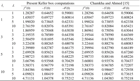
In order to assess the accuracy of numerical calculations, the present results compared for the special cases of Chamkha and Ahmed [15] whenPr=0.7, Nr=Nt=Nb=Sc=0, =1 1,
2 M 1 0.
= = = = = which depicts the Table 2 (nanofluid effects are negated in our model as are
[image:13.612.78.539.192.460.2]non-Boussinseq effect and magnetic field is neglected in the model of [15]). It is found that the present results are excellent agreement. Therefore confidence in the present Keller box code is justifiably high as testified to by validation of the present results.
Table 2. Comparison of local surface shear stresses and heat transfer coefficients.
1
Present Keller box computations Chamkha and Ahmed [15]
(0)
f −S(0) −(0) f(0) −S(0) −(0)
1
1 1.28287 0.64652 0.59001 1.28296 0.64658 0.59006 3 1.65037 0.69727 0.60814 1.65047 0.69723 0.60824 5 1.99020 0.73845 0.62331 1.99024 0.73855 0.62338 10 2.76159 0.82076 0.65391 2.76167 0.82084 0.65421
3
1 1.86959 0.75048 0.63038 1.86961 0.75056 0.63044 3 2.19535 0.78589 0.64358 2.19544 0.78590 0.64369 5 2.50459 0.81695 0.65546 2.50464 0.81700 0.65556 10 3.22438 0.88265 0.68078 3.22444 0.88276 0.68083
5
1 2.39989 0.82787 0.66175 2.39994 0.82790 0.66189 3 2.69928 0.85621 0.67256 2.69935 0.85626 0.67260 5 2.98723 0.88134 0.68225 2.98733 0.88146 0.68226 10 3.66796 0.93568 0.70429 3.66801 0.93576 0.70437
10
1 3.58371 0.96779 0.72198 3.58373 0.96785 0.72207 3 3.84386 0.98657 0.72929 3.84399 0.98667 0.72938 5 4.09821 1.00419 0.73610 4.09826 1.00427 0.73615 10 4.71131 1.04378 0.75212 4.71136 1.04383 0.75218
7. RESULTS AND DISCUSSION
A detailed parametric study has been performed for the influence of unsteadiness parameter
( )
A ,rotation parameter( )
,non-linear temperature parameter( )
1 ,Brownian motion parameter( )
Nb ,buoyancy ratio parameter( )
Nr ,thermophoretic parameter( )
Nt ,Prandtl number( )
Pr ,andSchmidt number
( )
Sc ,on dimensionless primary velocity( )
f ,secondary velocity( )
S ,temperature( )
,nanoparticle volume fraction( )
,primary and secondary skin friction functions, Nusseltnumber function and Sherwood number function. Table 3 depicts the Nusselt and Sherwood numbers for variousNbandNtwhen A=1,=0.5,Nr=0.5, Pr=0.71, Sc=0.6,1=1,1=0.5,Rex =1,
Br/*=1,/*=1and2 =0.1. It is noticed that increase in the thermophoresis leads to decrease in
parameter and progressively increasing Brownian motion parameter, there is a sustained depression in heat transfer rate whereas the mass transfer rate is elevated.
Table 3. Nusselt and Sherwood numbers for variousNbandNt.
Nb Nt −
( )
0 −( )
00.1
0.1 0.52958 0.30693 0.2 0.5165 0.11161 0.3 0.50374 -0.063 0.4 0.49131 -0.2178 0.5 0.47919 -0.3538 0.2
0.1
0.5116 0.42315 0.3 0.49402 0.46176 0.4 0.47685 0.48096 0.5 0.4601 0.4924
Table 4. Nusselt and Sherwood numbers for variousPrandSc. Pr Sc −
( )
0 −( )
01
1 0.41328 0.57186 2 0.38627 0.84516 5 0.35957 1.30073 10 0.34541 1.75771 2
2
0.34043 0.91972 5 0.16838 1.09872 10 0.04306 1.20955
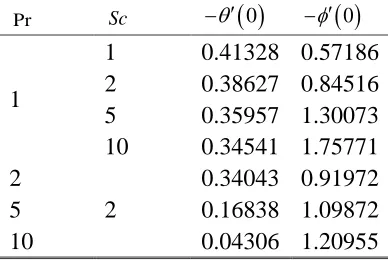
In Table 4, the Nusselt and Sherwood numbers for various Prandtl and Schmidt numbers are computed with A=1,=0.5, Nt=Nb=Nr=0.5, 1 =1, 1 =0.5, Rex =1, Br/*=1,/*=1 and
2 0.1.
= It is observed that as Schmidt number
( )
Sc rises nanoparticle volume fraction mass transfer [image:14.612.209.403.407.537.2]transferred to the sphere surface since greater temperatures result in the boundary layer. The nano-particle volume fraction is conversely reduced in the boundary layer and this is due to the greater transfer of nano-particles to the sphere surface (wall).
Table 5. Surface shear stresses, heat transfer rate and nanoparticle volume fraction rate.
1 Pr f
( )
0 −S( )
0 −( )
0 −( )
00.5 0.5
0.71 0.84921 0.55824 0.41537 0.40205 1 0.84906 0.55818 0.43643 0.39676 7 0.84864 0.558 0.24104 0.64109 10 0.84863 0.55799 0.15127 0.73171 0.5
0
0.71
0.84885 0.55816 0.41535 0.40205 1 0.84956 0.55831 0.41539 0.40207 2 0.85027 0.55846 0.41543 0.40209 1
0.5 0.71
0.95826 0.57765 0.42043 0.40496 2 1.16447 0.61185 0.4295 0.41014 5 1.719425 0.691501 0.451296 0.422484
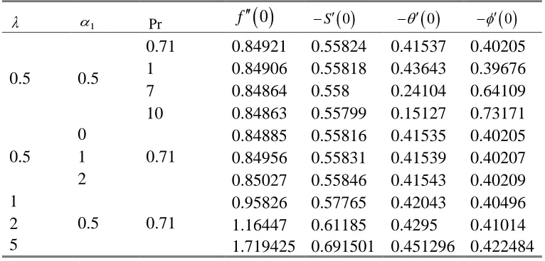
Table 5 presents the variation in primary and secondary surface shear stresses, heat transfer rate and nanoparticle volume fraction rate for different,1andPrwhenA=1, Nt=Nb=Nr=0.5, Sc=0.6,
1 0.5,
= Rex=1, Br/ =1, =/ 1and2 =0.1. The result indicates that as,1andPrincrease surface shear stresses
(
f(0),−S(0))
heat transfer rate(
− ( )
0)
and nano-particle mass transfer rate are all influenced. Primary shear stress is continuously enhanced with increasing rotation parameter () whereas secondary shear stress is initially decreased and then only weakly increased with subsequent increase in . With increasing non-linear parameter all variables are enhanced. We note that the Boussineq case is retrieved for 1 = 0 and this under-predicts the heat transferrate compared with the non-Boussineq case (1 > 0). With increasing Prandtl number, primary and
secondary shear stress and also heat transfer rate are all reduced, whereas nano-particle mass transfer rate is initially reduced and thereafter significantly enhanced. To provide additional insight about the effects of,1andPrinto the under studied problem, the graphical results will be discussed hereafter.
Comprehensive solutions have been obtained and their respective profiles are presented graphically for primary and secondary velocity components
(
f S,)
,temperature( )
andnanoparticle volume fraction
( )
in Figs. 2 – 10. Moreover, Figs. 11 – 12 depict the influence of selected parameters on entropy generation number, local Nusselt number and local Sherwood numbers. In the present computations, the following default parameters are prescribed (unless otherwise stated): A=1,=0.5, Nt=Nb=Nr=0.5,Pr=0.71, Sc=0.6,1=1,1=0.5,Rex=1, Br/ =1,/ 1
= and2 =0.1.
Figs. 3(a)-3(b) reveals the influence of unsteadiness parameter on the fluid velocity profiles
(
f S,)
,temperature( )
and nanoparticle volume fraction( )
profiles. It is observed that from Fig. 3(a) increase in unsteadiness (acceleration) parameterAresults in an increase in the primarymomentum is re-distributed via rotation of the sphere which is accelerating in the primary direction for A>0. Hence, the fluid inside the boundary layer is accelerated in the x-direction and decelerated in the rotational (secondary) direction. From Fig. 3(b) it is observed that both temperature
( )
and nanoparticle volume fraction( )
profiles are depressed with increasing values ofA, implying that both thermal and concentration boundary layers are depressed with increasing unsteadiness. The boundary layer will therefore be cooled and more heat and nano-particles transferred to the sphere surface (wall) with increasing unsteadiness effect.Figs. 4(a)-4(b) shows the influence of rotating parameter
( )
on primary and secondary velocity components(
f S,)
(i.e. x- direction and z- direction velocities), temperature( )
andnanoparticle volume fraction
( )
. Increasing λ, the rotation becomes more intense and the secondary momentum contributes more to the primary momentum via the swirl effect. This accelerates the primary flow and retards the secondary flow. Conversely greater rotation depresses magnitudes of temperature and nanoparticle concentration manifesting in a reduction in thermal and nano-particle concentration boundary layer thicknesses. In all cases asymptotically smooth profiles are computed in the free stream indicating that a sufficiently large infinity boundary condition is prescribed in the Keller box numerical code.Figs. 5(a)-5(b) demonstrates the influence of mixed convection parameter
( )
1 in buoyancy-assisted flow on the primary velocity
( )
f and secondary velocity( )
S , temperature( )
andnanoparticle volume fraction
( )
. The primary velocity is accelerated significantly whereas the secondary velocity is retarded for increasing mixed convection parameter1. A primary velocityovershoot is observed with very high mixed convection parameter
( )
1 which may be attributableto the strong buoyancy force for low Prandtl number fluid. The assisting buoyancy force acts like a favorable pressure gradient and accelerates the primary flow considerably. The temperature profiles are depressed for increasing mixed convection parameter1indicating that an accentuation
in thermal buoyancy force has an inhibitive effect on temperature. Conversely increasing mixed convection parameter boosts concentration of nano-particles in the boundary layer. Stronger thermal buoyancy cools and thins the thermal boundary layer whereas it thickens the nano-particle concentration boundary layer.
Fig. 6(a)-6(b) demonstrates the influence of non-linear temperature (or non-Boussinesq) parameter1on primary and secondary velocity profiles
(
f S,)
, temperature and nanoparticlevolume fraction distributions. It is observed that increasing 1 the primary velocity is markedly
accelerated and nano-particle concentration is elevated. However secondary velocity is decelerated and temperature is reduced with greater non-Boussinesq parameter. The Boussinesq case (1 = 0)
therefore over-predicts the secondary velocity whereas it under-predicts the primary velocity. Also the Boussinesq case tends to under-predict nano-particle concentration whereas it over-predicts the temperature. Significant deviation from the Boussinesq case is computed with increasing values of the nonlinear temperature parameter is progressively stronger non-Boussinesq case (1 > 0). These findings concur with other studies including Kameswaran et al. [8] and Partha [21]
indicating that the non-Boussinesq model exerts a non-trivial effect on thermofluid transport phenomena.
Figs. 7(a)-7(b) depict the effect of the Schmidt number
( )
Sc on primary and secondaryvelocity components
(
f S,)
, temperature and nanoparticle volume fraction profiles. Withreduced weakly. Schmidt number is the ratio of momentum diffusivity to mass (nano-particle) diffusivity. For Sc < 1 mass diffusivity exceeds momentum diffusivity and vice versa for Sc >1. Temperature magnitudes are weakly decreased whereas nanoparticle volume fraction magnitudes are greatly increased with greater values of Schmidt number. Concentration boundary layer thickness for nano-particle species is significantly elevated with greater Schmidt number whereas the thermal boundary layer thickness is slightly decreased.
Figs. 8(a)-8(c) demonstrate the effect of the Brownian motion parameter (Nb) primary and secondary velocity components i.e. fandS, temperature
( )
and nanoparticle volume fraction( )
for Prandtl numbers 0.71 (air based) and 7 (water based) nanofluids. Increasing Nbinduces a strong rise in primary velocity and temperature profiles whereas it results in a strong decrease in secondary velocity and nanoparticle volume fraction (concentration) for both air and water based nanofluids. Larger Nb values correspond to smaller nano-particles [2] and this encourages acceleration of the primary flow. However it results also in a reduction in diffusion of nano-particles and a decrease in concentration boundary layer thickness. In Figs. 8a-c it is also observed that Prandtl number increment (Pr = 0.71 for gas based nanofluids and Pr = 7 for water based nanofluids) reduces primary velocity and temperature whereas it enhances secondary velocity and very substantially enhances particle concentration. With larger Prandtl number the nano-particle concentration boundary layer thickness is increased whereas the thermal boundary layer thickness is depleted. Similar observations have been computed by Srinivasacharya and Surender [9] and also Zheng et al. [34].Figs. 9(a)-9(b) illustrate the effects of buoyancy ratio (Nr) and Prandtl number (Pr) on
primary and secondary velocity profiles
(
f S,)
, temperature( )
and nanoparticle volume fraction( )
. With increasing buoyancy ratio, primary velocity is strongly depressed whereas the secondary velocity is increased. However positive values are sustained for secondary velocity throughout the boundary layer indicating that back flow (flow reversal) never arises. Higher Nr values also generally result in an increase in temperature( )
and decrease in nanoparticle volume fraction( )
profiles. When Prandtl number increases the primary velocity( )
f decreases whereas the secondary velocity increases. Furthermore there is a strong elevation in temperatures with higher Prandtl number whereas there is a plummet in nano-particle concentration magnitudes.Figs. 10(a)-10(c) demonstrates the effect of thermophoresis parameter
( )
Nt and Prandtl number( )
Pr on primary and secondary velocity(
f S,)
temperature and concentration distributions. Increasing the thermophoresis effect decreases the primary velocity whereas it elevates secondary velocity. An increase in Prandtl number a significant reduction in primary velocity occurs whereas a weak decrease in secondary velocity arises. IncreasingNt tends to increase both temperature and nano-particle concentration magnitudes. Increasing Prandtl number decreases temperature profiles whereas it substantially boosts nano-particle concentration profiles. Greater thermophoresis implies stronger migration of nano-particles under a temperature gradient away from the sphere surface. This increases nano-particle concentration in the boundary layer and therefore also concentration boundary layer thickness.Fig. 11(a) shows that the effect of non-linear temperature parameter (1), for both cases of
gas-based nanofluid (Pr=0.71) and water-based nanofluid (Pr=7), on entropy generation number
( )
Ng . It is observed that NG increases with increases of non-linear temperature parameter i.e.greater Prandtl number (lower thermal conductivity of nanofluid). Fig. 11(b) indicates that magnitudes of entropy generation number increase with an increase in the viscous dissipation parameter (Br/*). For Br/* =0 viscous heating effects are neglected. With greater
(
Br/)
i.e. increasing Brinkman number the slower the conduction of heat produced by viscous dissipation and hence the larger the temperature rise. This also increases nanofluid friction and results in a boost in entropy generation. In all cases entropy generation is found to be maximized at the sphere surface (wall). The influence of the local Reynolds number on entropy generation number( )
Ng ispresented in Fig 11(c). An increase in local Reynolds number corresponds to greater inertial force contribution which boosts the momentum in the boundary layer and increases Ng values. It will also be accompanied by higher heat transfer rates at the surface of the rotating sphere. Fig. 11(d)
depicts the influence of unsteadiness
( )
A on entropy generation number. It is observed that Ngincreases with unsteadiness i.e. acceleration parameter and again this is associated with the greater contribution of inertial force to the regime. Generally higher values of entropy generation are computed with increasing Prandtl number.
Figs. 12(a-c), present the variation in surface heat transfer rate i.e. Nusselt number
(
− ( )
0)
and surface mass transfer rate i.e. Sherwood number
(
−( )
0)
plotted against thermophoresis parameter (Nt) for different values of Brownian motion parameter (Nb) and nonlinear temperature parameter (1). Evidently inspection of Fig 12 (a) reveals that a strong elevation in surface heattransfer rate accompanies an increase in Brownian motion parameter whereas a weaker elevation in nano-particle volume fraction mass transfer rate is computed. Generally larger Nb values i.e. smaller nano-particle size encourages both heat and mass transfer to the sphere surface, confirming the results described earlier in Table 3. With increasing linear temperature parameter (i.e. non-Boussinesq case, 1 =0.5), both heat transfer and mass transfer rates are enhanced compared with
the Boussinesq case (1 =0). With increasing thermophoresis parameter (Nt) there is a general
decline in both heat transfer rate and mass transfer rate, although the reduction in the former is more significant. Figs. 12(b-c) depict the effects of the acceleration parameter (A) and rotation parameter () on the local reduced Nusselt and Sherwood numbers and primary and secondary surface shear stress coefficients. Both Nusselt number and Sherwood number are found to be enhanced with rotation (swirl) and unsteadiness (acceleration) parameter, although significantly higher magnitudes are computed for Nusselt number. Primary and secondary shear stress (skin friction) coefficients are also increased as the acceleration parameter and rotation parameters increase, indicating that stronger thermal buoyancy and unsteadiness effects accelerate both primary and secondary flow, although much larger magnitudes are as expected associated with the primary flow.
8. CONCLUSIONS
Furthermore a gird-independence study has been conducted. The main deductions from the present computations can be summarized as follows:
➢ Increasing unsteadiness (acceleration) parameter elevates the primary velocity component, primary shear stress coefficient, local reduced Nusselt and Sherwood numbers whereas it decreases secondary velocity component, temperature and nano-particle concentration.
➢ With greater non-linear temperature parameter (i.e. non-Boussinesq case), both heat transfer and mass transfer rates are increased compared with the Boussinesq case.
➢ With increasing thermophoresis parameter there is a decrease in heat transfer rate (Nusselt number) and mass transfer rate (Sherwood number).
➢ An increase in non-linear temperature parameter (non-Boussinesq effect), Brinkman number (viscous dissipation parameter) and local Reynolds number increases entropy generation number whereas increasing Prandtl number reduces it.
➢ Irreversibility is reduced to a great extent by using nanofluids i.e. with the presence of nano-particles.
➢ Primary and secondary shear stress (skin friction) coefficients, Nusselt number and Sherwood number are increased with rotation parameter.
➢ Temperature is reduced whereas nanoparticle concentration is increased strongly with an increase in Schmidt number.
➢ With increasing buoyancy ratio, primary velocity and nano-particle concentration are reduced whereas secondary velocity and temperature are increased.
➢ Increasing Brownian motion parameter elevates both primary velocity and temperature profiles whereas it reduces secondary velocity and nanoparticle volume fraction (concentration) for both air and water based nanofluids.
➢ With increasing mixed convection parameter, primary velocity is accelerated and nano-particle concentration is enhanced whereas secondary velocity is decelerated and temperatures are reduced.
The present study may be further extended to consider non-Newtonian e.g. viscoelastic fluid characteristics and non-Fourier heat conduction effects [35]. These are also of relevance in chemical engineering.
Conflicts of Interest: The authors declare no conflict of interest.
ACKNOWLEDGEMENTS
Fig. 3(a) Effect of dimensionless unsteadiness parameter (A) on primary (f /) and
secondary (S) velocities.
Fig. 3(b) Effect of unsteadiness parameter (A) on temperature () and nanoparticle volume fraction i.e. concentration ().
0 0.25 0.5 0.75 1 1.25
0 3 6
9 12 15A= 0.8, 1, 1.3, 1.7, 2, 2.5.
f'
S
0
0.25
0.5
0.75
1 0
0.25 0.5 0.75 1
0 1 2 3 4 5
Fig. 4(a) Effect of dimensionless rotation parameter () on primary (f /) and secondary
(S) velocities.
.
Fig. 4(b) Effect of dimensionless rotation parameter () on temperature () and nanoparticle volume fraction i.e. concentration ().
0 0.4 0.8 1.2
0 1 2 3
s
= 0.1, 0.5, 5, 10, 20.
f'
S f'
0
0.2
0.4
0.6
0.8
1 0
0.2 0.4 0.6 0.8 1
0 1 2 3 4 5
Fig. 5(a) Effect of mixed convection parameter (1) on primary (f /) and secondary (S)
velocities.
Fig. 5(b) Effect of mixed convection parameter (1) on temperature () and nanoparticle volume fraction i.e. concentration ().
.
0 0.25 0.5 0.75 1
0 1 2 3
f
s
1= 0, 0.1, 0.5, 1, 2, 5. .
f'
S
0
0.25
0.5
0.75
1 0
0.25 0.5 0.75 1
0 1 2 3 4 5
1= 0, 0.1, 0.5, 1, 2, 5. .
-Fig. 6(a) Effect of non-linear temperature parameter (1) on primary (f /) and secondary
(S) velocities.
Fig. 6(b) Effect of non-linear temperature parameter (1) on temperature () and nanoparticle volume fraction i.e. concentration ().
.
0 0.25 0.5 0.75 1
0 2 4
f
'
s
1= 0, 0.1, 0.5, 1, 2, 5, 10. .
f'
S
0
0.25
0.5
0.75
1 0
0.25 0.5 0.75 1
0 1 2 3 4 5
1= 0, 0.1, 0.5, 1, 2, 5, 10. .
Fig. 7(a) Effect of Schmidt number (Sc) on primary (f /) and secondary (S) velocities.
.
Fig. 7(b) Effect of Schmidt number (Sc) on temperature () and nanoparticle volume fraction i.e. concentration ().
.
0 0.25 0.5 0.75 1
0 2 4
f
,
s
Sc= 0.2, 0.6, 0.9, 2, 2.5. .
f'
S
0
0.25
0.5
0.75
1 0
0.25 0.5 0.75 1
0 1 2 3 4 5 6 7
Sc= 0.2, 0.6, 0.9, 2, 2.5.
Fig. 8(a) Effect of Brownian motion parameter (Nb) and Prandtl number (Pr) on primary (f /) and secondary (S) velocities.
Fig. 8(b) Effect of Brownian motion parameter (Nb) on temperature () for various Pr.
0 0.25 0.5 0.75 1
0 1 2 3
Nb= 0.1, 0.2, 0.3, 0.5, 0.7, 1.
f'
S Pr =0.71
Pr = 7.0 f'
S
0 0.25 0.5 0.75 1
0 1 2 3 4
Pr =0.71
Nb= 0.1, 0.2, 0.3, 0.5, 0.7, 1.
Fig. 8(c) Effect of Brownian motion parameter (Nb) on nanoparticle volume fraction i.e. concentration () for various Prandtl numbers (Pr).
Fig. 9(a) Effect of buoyancy ratio parameter (Nr) and Prandtl number (Pr) on the primary (f /) and secondary (S) velocities.
0 0.5 1 1.5 2 2.5
0 2 4
Pr =0.71 Pr = 7
Nb= 0.1, 0.2, 0.3, 0.5, 0.7, 1.
0 0.25 0.5 0.75 1
0 1 2 3 4
f
s
Pr= 0.71
Pr= 7
Nr = 0, 0.2, 0.3, 0.5, 0.7, 1.
f'
Fig. 9(b) Effect of buoyancy ratio parameter (Nr) and Prandtl number (Pr) on temperature () and nanoparticle volume fraction i.e. concentration ().
Fig. 10(a) Effect of thermophoresis parameter (Nt) and Prandtl number (Pr) on the primary (f /) and secondary (S) velocities.
.
0
0.25
0.5
0.75
1 0
0.25 0.5 0.75 1
0 1 2 3 4 5
Pr =0.71
Nr = 0, 0.2, 0.3, 0.5, 0.7, 1..
Pr= 7
0 0.25 0.5 0.75 1
0 1 2 3 4
f
s
Pr= 0.71
Nt= 0, 0.2, 0.3, 0.5, 0.7, 1.
Pr= 7
f'
Fig. 10(b) Effect of thermophoresis parameter (Nt) and Prandtl number (Pr) on temperature ().
Fig. 10(c) Effect of thermophoresis parameter (Nt) on nano-particle volume fraction i.e. concentration () for various Prandtl numbers (Pr).
0 0.25 0.5 0.75 1
0 1 2 3 4 5
Pr=0.71
Nt= 0, 0.2, 0.3, 0.5, 0.7, 1.
Pr= 7
0 0.25 0.5 0.75 1
0 2
4
Pr=0.71
Pr= 7
Fig.11(a) Effect of non-linear temperature parameter ( 1) on entropy generation
number (Ng) for various Prandtl numbers (Pr).
Fig.11(b) Influence of Br/* on entropy generation number (Ng).
0 1 2 3 4 5
0 1.5 3
Ng
1= 0, 0.2, 0.5, 1, 1.5, 2.
Pr= 7
Pr= 0.71
0 3 6 9 12 15 18 21
0 1 2 3
Ng
Fig.11(c) Influence of local Reynolds number (Rex) on entropy generation number (Ng).
Fig.11(d) Influence of unsteadiness parameter (A) on entropy generation number (Ng). for various Prandtl numbers (Pr).
.
0 2.5 5 7.5 10
0 1 2 3
Ng
Rex= 0, 0.1, 0.5, 1, 2, 5.
0 3 6 9
0 1 2
Ng
A= 0.8, 1, 1.5, 2
Pr= 7
Fig.12(a) Effects of non-linear temperature (1), Brownian motion (Nb) and thermophoresis parameter (Nt) on reduced Nusselt number (-()) and reduced Sherwood number (-() ).
Fig.12(b) Effects of mixed convection parameter () and unsteadiness parameter (A) on reduced Nusselt number (-()) and reduced Sherwood number (-() ).
0.4 0.65 0.9 1.15
0.2 0.45 0.7 0.95
-
()
−
()
Nt
-()
-()
Nb= 0.1
Nb= 0.3
Nb= 0.5
z
1 =
1= .5
0.2 0.3 0.4 0.5 0.6 0.7
0.6 0.8 1 1.2 1.4 1.6 1.8 2
-
(0)
,
-
(0)
A
= 1, 3, 5, 10.
-(0)
Fig.12(c) Effects of mixed convection parameter () and unsteadiness parameter (A) on primary (f //(0)) and secondary (-S/(0)) skin friction coefficients.
REFERENCES
[1] Choi, SUS, Enhancing thermal conductivity of fluids with nanoparticles in developments and Applications of Non-Newtonian Flows, D. A Springer and H. P. Wang, Eds., ASME, 1995; 66: 99-105.
[2] Buongiorno, J., Convective transport in nanofluids, ASME J. Heat Transfer, 2006;128: 3: 240-250.
[3] Zan Wu, Lei Wang, and Bengt Sundén, Pressure drop and convective heat transfer of water and nanofluids in a double-pipe helical heat exchanger, Applied Thermal Engineering, 2013; 60: 266-274.
[4] Ulzie Rea, Tom McKrell, Lin-Wen Hu and J. Buongiorno, Laminar convective heat transfer and viscous pressure loss of alumina–water and zirconia–water nanofluids, Int. J. Heat and Mass Transfer, 2009; 52:2042-2048.
[5] Das, SK, Choi, SU, Yu W and Pradeep T, Nanofluids: Science and Technology. John Wiley, New Jersey, 2007.
[6] Kuznetsov, AV and Nield, DA, Natural convective boundary-layer flow of a nanofluid past a vertical plate, International Journal of Thermal Sciences, 2010; 49(2): 243-247.
-0.6 0.4 1.4 2.4 3.4
0.6 0.8 1 1.2 1.4 1.6 1.8 2
f'
'(
0
),
-S'
(0
)
A
= 1, 3, 5, 10.
[7] Gorla, RSR and Hossain A, Mixed convective boundary layer flow over a vertical cylinder embedded in a porous medium saturated with a nanofluid, International Journal of Numerical Methods for Heat and Fluid Flow, 2013;23(8):1393-1405.
[8] Kameswaran, PK, Vasu B., Murthy PVSN and Gorla RSR, Mixed convection from a wavy surface embedded in a thermally stratified nanofluid saturated porous medium with non-linear Boussinesq approximation, International Communications in Heat and Mass Transfer, 2016;77:78-86.
[9] Srinivasacharya D, and Surender O, Mixed convection boundary layer flow of a nanofluid past a vertical plate in a doubly stratified porous medium, Journal of Computational and Theoretical Nanoscience, 2014;11(8):1853-1862.
[10] Bég, O. Anwar, Md. Faisal Md Basir, M. J. Uddinand A. I. Md. Ismail, Numerical study of slip effects on unsteady asymmetric bioconvective nanofluid flow in a porous microchannel with an expanding/contracting upper wall using buongiorno’s model, J. Mech. Med. Biol. 0, 1750059 (2016) [28 pages]. DOI: http://dx.doi.org/10.1142/ S0219519417500592
[11] Murthy PVSN, Ram Reddy C, Chamkha AJ, and Rashad AM, Significance of viscous dissipation and chemical reaction on convective transport in a boundary layer stagnation point flow past a stretching/shrinking sheet in a nanofluid Journal of Nanofluids, 2015;4: 214-222. [12] Gorla RSR, and Vasu B, Unsteady convective heat transfer to a stretching surface in a non-Newtonian nanofluid, Journal of Nanofluids 2016; 5(4): 581-594.
[13] Takhar HS, and Nath G, Self-similar solution of the unsteady flow in the stagnation point region of a rotating sphere with a magnetic field, Heat and Mass Transfer, 2000; 36(2):. 89-96. [14] Anilkumar D. and Roy S, Self-similar solution of the unsteady mixed convection flow in the stagnation point region of a rotating sphere, Heat and Mass Transfer, 2004;40(6):487-493. [15] Anwar Bég, O., Prasad, V.R., Vasu, B., R.S.R. Gorla, Computational modeling of magnetohydrodynamic convection from a rotating cone in orthotropic Darcian porous media, J. Braz. Soc. Mech. Sci. Eng. (2017). doi:10.1007/s40430-017-0708-x
[16] Chamkha AJ and Ahmed SE, Unsteady MHD heat and mass transfer by mixed convection flow in the forward stagnation region of a rotating sphere at different wall conditions, Chemical Engineering Communications, 2012;199(1): 122-141.
[17] Bég O. Anwar, Mabood F and Nazrul Islam M, Homotopy simulation of nonlinear unsteady rotating nanofluid flow from a spinning body, Int. J. Engineering Mathematics, 2015: Article ID 272079, 15 pages. http://dx.doi.org/10.1155/2015/272079