BIROn - Birkbeck Institutional Research Online
Sturm, P.F. and Maybank, Stephen J. (1999) On plane-based camera
calibration:
a
general
algorithm,
singularities,
applications.
In:
UNSPECIFIED (ed.) Proceedings, 1999 IEEE Computer Society Conference
on Computer Vision and Pattern Recognition.
Hoboken, U.S.:
IEEE
Computer Society, pp. 432-437. ISBN 0769501494.
Downloaded from:
Usage Guidelines:
Please refer to usage guidelines at
or alternatively
On Plane-Based Camera Calibration:
A General Algorithm, Singularities, Applications
Peter F. Sturm and Stephen J. Maybank
Computational Vision Group, Department of Computer Science
The University of Reading
Whiteknights, PO Box 225
Reading, RG6 6AY, United Kingdom
{
P.F.Sturm, S.J.Maybank
}
@reading.ac.uk
ACCEPTED FORCVPR’99. VERSION OFNOVEMBER18, 2015.Abstract
We present a general algorithm for plane-based calibration that can deal with arbitrary numbers of views and calibration planes. The algorithm can simultaneously calibrate different views from a camera with variable intrinsic parameters and it is easy to incorporate known values of intrinsic parameters. For some minimal cases, we describe all singularities, naming the parameters that can not be estimated. Experimental results of our method are shown that exhibit the singularities while reveal-ing good performance in non-sreveal-ingular conditions. Several applications of plane-based 3D geometry inference are discussed as well.
1
Introduction
The motivations for considering planes for calibrating cameras are mainly twofold. First, concerning calibration in its own right, planar calibration patterns are cheap and easy to produce, a laser printer output for example is absolutely sufficient for applications where highest accuracy is not demanded. Second, planar surface patches are probably the most important twodimensional “features”: they abound, at least in man-made environments, and if their metric structure is known, they carry already enough information to determine a camera’s pose up to only two solutions in general [3]. Planes are increasingly used for interactive modeling or measuring purposes [1, 9, 10].
The possibility of calibrating cameras from views of planar objects is well known [6, 11, 13]. Existing work however, restricts in most cases to the consideration of a single or only two planes (an exception is [7], but no details on the algorithm are provided) and cameras with constant calibration. In addition, the study of singular cases is usually neglected (besides in [11] for the simplest case, calibration of the aspect ratio from one view of a plane), despite their presence in common configurations. It is even possible for cameras to self-calibrate from views of planar scenes with unknown metric structure [12], however several views are needed (Triggs recommends up to 9 or 10 views of the same plane for reliable results) and the “risk” of singularities should be greater compared to calibration from planes with known metric structure.
In this paper, we propose a general algorithm for calibrating a camera with possibly variable intrinsic parameters and posi-tion, that copes well with an arbitrary number of calibration planes (with known metric structure) and camera views. Calibration is essentially done in two steps. First, the 2D-to-2D projections of planar calibration objects onto the image plane(s) are com-puted. Each of these projections contributes to a system of homogeneous linear equations in the intrinsic parameters, which are hence easily determined. Calibration can thus be achieved using only linear operations (solving linear equations), but can of course be enhanced by subsequent non linear optimization.
The paper is organised as follows: in§2, we describe the camera model used and the representation of projections of planar objects. In§3, we introduce the principle of plane-based calibration. A general algorithm is proposed in§4. Singularities are revealed in§5. Experimental results are presented in§6, and some applications described in§7.
2
Background
Camera Model. We use perspective projection to model cameras. A projection may be represented by a3×4projection matrixPthat maps points of 3-space to points in 2-space: q ∼ PQ. Here, ∼means equality up to a non zero scale factor, which accounts for the use of homogeneous coordinates. The projection matrix incorporates nicely the so-called extrinsic and intrinsic camera parameters; it may be decomposed as:
P∼KR( I3 | −t) , (1)
whereI3 is the3×3 identity matrix, Ra3 ×3 orthogonal matrix representing the camera’s orientation, ta 3-vector
K=
τ f s u0
0 f v0
0 0 1
.
In general, we distinguish 5 intrinsic parameters for the perspective projection model: the (effective) focal lengthf, the aspect ratioτ, the principal point(u0, v0)and the skew factorsaccounting for non rectangular pixels. The skew factor is
usually very close to0, so we ignore it in the following.
Calibration and Absolute Conic. Our aim here is to calibrate a camera, i.e. to determine its intrinsic parameters or its calibration matrixK(subsequent pose estimation is relatively straightforward). Instead of directly determiningK, we will try to compute the symmetric matrixKKTor its inverse, from which the calibration matrix can be computed uniquely using Cholesky
decomposition. As will be seen, this approach leads to simple and, in particular, linear calibration equations.
Furthermore, the analysis of singularities of the calibration problem is greatly simplified: the matrixω ∼ (KKT)−1 =
K−TK−1represents the image of the Absolute Conic whose link to calibration and metric scene reconstruction is exposed for example in [2]. This geometrical view helps us with the derivation of singular configurations (cf.§5).
Planes, Homographies and Calibration. In this paper, we consider the use of one or several planar objects for calibration. When we talk aboutcalibration planes, we mean the supports of planar calibration objects. The restriction of perspective projection to points (or lines) on a specific plane takes on the simple form of a3×3homography. This homography depends on the relative positioning of camera and plane and the camera’s intrinsic parameters. Without loss of generality, we may suppose that the calibration plane coincides with the planeZ = 0of some global reference frame. This way, the homography can be derived from the full projection matrixPby dropping the third column in equation (1), that has no effect here:
H∼KR
1 0 0 1 −t 0 0
. (2)
The homography can be estimated from four or more point or line correspondences between the plane and the camera’s image plane. It can only be sensibly decomposed as shown in equation (2), if the metric structure of the plane is known (up to scale is sufficient), i.e. if the coordinates of points and lines used for computingHare known in a metric frame. For our purposes, we mainly use corner points of rectangles with known edge lengths, to compute the homographies.
Equation (2) suggests that the 8 coefficients ofH(9 minus 1 for the arbitrary scale) might be used to estimate the 6 pose parametersRandt, while still delivering 2 constraints on the calibrationK. These constraints allow us to calibrate the camera, either partially or fully, depending on the number of calibration planes, the number of images, the number of intrinsic parameters to be computed and on singularities.
3
Principle of Plane-Based Calibration
Calibration will be performed via the determination of the image of the Absolute Conic (IAC),ω ∼K−TK−1, using plane
homographies. As mentioned previously, we consider pixels to be rectangular, and thus the IAC has the following form (after appropriate scaling):
ω∼
1 0 −u0
0 τ2 −τ2v
0
−u0 −τ2v0 τ2f2+u20+τ2v20
. (3)
The calibration constraints arising from homographies can be expressed and implemented in several ways. For example, it follows from equation (2) that:
HTωH∼HTK−TK−1H∼
1 0 −t1
0 1 −t2
−t1 −t2 tTt
.
The camera positiontbeing unknown and the equation holding up to scale only, we can extract exactly two different equations inωthat prove to be homogeneous linear:
hT1ωh1−hT2ωh2 = 0 (4)
wherehiis theith column ofH.
These are our basic calibration equations. If several calibration planes are available, we just include the new equations into a linear equation system. It does not matter if the planes are seen in the same view or in several views or if the same plane is seen in several views, provided the calibration is constant (this restriction is relaxed in the next section). The equation system is of the formAx=0, with the vector of unknownsx= (ω11, ω22, ω13, ω23, ω33)
T
.
Before solving the linear equation system, attention has to be paid to numerical conditioning (see§4.3). After having determinedω, the intrinsic parameters are extracted via:
τ2 = ω22 ω11
(6)
u0 = −
ω13
ω11
(7)
v0 = −
ω23
ω22
(8)
f2 = ω11ω22ω33−ω22ω
2
13−ω11ω223
ω11ω222
(9)
4
A General Calibration Algorithm
We describe now how the basic principle of plane-based calibration exposed in the previous section can be extended in two important ways. First, we show that prior knowledge of intrinsic parameters can be easily included in the linear estimation scheme. Second, and more importantly, we show how the scheme can be applied for calibrating cameras with variable intrinsic parameters.
4.1
Prior Knowledge of Intrinsic Parameters
Letaibe theith column of the design matrixAof the linear equation system described in the previous section. We may
rewrite the equation system as:
ω11a1+ω22a2+ω13a3+ω23a4+ω33a5=0 .
Prior knowledge of, e.g. the aspect ratioτ, allows us via equation (6) to eliminate one of the unknowns, sayω22, leading to the
reduced linear equation system:
ω11(a1+τ2a2) +ω13a3+ω23a4+ω33a5=0 .
Prior knowledge ofu0orv0can be dealt with similarly. The situation is different for the focal lengthf, due to the complexity
of equation (9): prior knowledge of the focal length allows to eliminate unknowns only if the other parameters are known, too. However, this is not much of a problem – it is rarely the case that the focal length is known beforehand while the other intrinsic parameters are unknown.
4.2
Variable Intrinsic Parameters
We make two assumptions about possible variations of intrinsic parameters, that are not very restrictive but eliminate some useless special cases to deal with. First, we consider the aspect ratio to be constant for a given camera. Second, the principal point may vary, but only in conjunction with the focal length. Hence, we consider two modes of variation in intrinsic parameters: onlyfvaries orf, u0andv0vary together (it is straightforward to develop the case of only one coordinate of the principle point
being variable).
If we take into account the calibration equations arising from a view for which it is assumed that the intrinsic parameters have changed with respect to the preceding view (e.g. due to zooming), we just have to introduce additional unknowns inxand columns inA. If only the focal length is assumed to have changed, a new unknownω33is needed. If in addition the principal
point is supposed to have changed, we add also unknowns forω13andω23(cf. equation (3)). The corresponding coefficients
of the calibration equations have to be placed in additional columns ofA.
Note that the consideration of variable intrinsic parameters does not mean that we have to assume different values forall
views, i.e. there may be sets of views sharing the same intrinsics, sharing only the aspect ratio and principal point, or sharing the aspect ratio alone. The integration of variable intrinsic parameters and such that are known beforehand for some views, as described above, is trivial as well.
4.3
Complete Algorithm
The input to the calibration algorithm consists of:
• Feature correspondences (usually points or lines) between planar objects and views. The plane features have to be given in a metric frame.
• Known values of intrinsic parameters. They may be provided for individual views and any of the parametersτ, u0orv0
independently.
• Flags indicating for individual intrinsic parameters if they stay constant or vary across different views.
The complete algorithm consists of the following steps:
1. Compute plane homographies from the given features.
2. Construct the equation matrixA(cf.§§4.1 and 4.2).
3. Ensure good numerical conditioning ofA(see below).
4. Solve the equation system by any standard numerical method and extract the values of intrinsic parameters from the solution as shown in equations (6) to (9).
Conditioning. We may improve the conditioning of Aby the standard technique of rescaling rows and columns [4]. In practice, we omit row-wise rescaling for reasons explained below. Columns are rescaled by post-multiplyingAby a diagonal matrixT: A0 =AT. The matrixTis chosen such as to make the norms of the columns ofA0of approximately equal order of
magnitude. From the solutionx0of the modified equation systemA0x0 =0we obtain the solutionxof the original problem as:x=T−1x0. This column-wise rescaling is crucial to obtain reliable results.
As for rescaling rows, this proves to be delicate in our case, since occasionally there are rows with all coefficients very close to zero. Scaling these rows such as to have equal norm as others will hugely magnify noise and lead to unreliable results. A possible solution would be to edit coefficients that are very close to zero.
Comments. The described calibration algorithm requires mainly the solution of a single linear equation system. The solution
xis usually determined as the vector minimizing the algebraic error|Ax|. Naturally, the solution may be optimized subse-quently using non linear least squares techniques. This optimization should be done simultaneously for the calibration and the pose parameters, that may be initialized in a straightforward manner from the linear calibration results. For higher accuracy, optical distortions should be taken into account. Distortion coefficients might be computed right from the start using the plane homographies, or as part of the final optimization.
Minimal Cases. In general, each view of a calibration object provides two calibration equations. In the absence of singulari-ties, the number of intrinsic parameters that can be estimated uniquely, equals the total number of equations. So, for example, with a single view of a single plane, we might calibrate the aspect ratio and focal length, provided the principal point is given. Two views of a single plane, or one view of two planes is sufficient to fully calibrate the camera. Another interesting minimal case is about three views of a single plane, where the views are taken by a zooming camera: with a total of 6 equations we might determine the 3 focal lengths, the aspect ratio and the principal point.
5
Singularities
The successful application of any algorithm requires awareness of singularities. This enables avoiding situations where the result is expected to be unreliable or restricting the problem at hand to a solvable one. In the following we describe the singularities of calibration from one or two planes.
Due to lack of space, we are only able to give a sketch of the derivations. A first remark is that only the relative orientation of planes and camera is of importance for singularities, i.e. the position and the actual intrinsic parameters do not influence the existence of singularities. A second observation is that planes that are parallel to each other provide exactly the same information as a single plane with the same orientation (except that more feature correspondences may provide a higher robustness in practice). So, as for the case of two calibration planes, we omit dealing with parallel planes and instead refer to the one-plane scenario.
satisfies the calibration equations (4) and (5), contains the projections of the circular points of the calibration planes. Naturally, this is also valid forω0. If we exclude the planes of being parallel to each other (cf. the above discussion), the two lines making upω0 are nothing else than the vanishing lines of the calibration planes. There is one point left to consider: since we are
considering rectangular pixels, the IAC is required to be of the form (3), i.e. its coefficientω12has to be zero. Geometrically,
this is equivalent to the conic being symmetric with respect to a vertical and a horizontal line (this is referred to as “reflection constraint” in table 2). Based on these considerations, it is a rather mechanical task to derive all possible singularities.
All singularities for one-plane and two-plane calibration and for different levels of prior knowledge are described in tables 1 and 2. In addition, we reveal which of the intrinsic parameters can/can’t be estimated uniquely. The tables contain columns for
τ fandf which stand for the calibrated focal length, once measured in horizontal, once in vertical pixel dimensions. In some cases it is possible to compute, e.g.τ f, without the possibility of determiningτorf individually.
A general observation is that a plane that is parallel to the image plane, allows to estimate the aspect ratio, but no other parameters. A general rule is that the more regular the geometric configuration is, the more singularities may occur.
Prior Pos. of calibration plane τ τ f f u0 v0 u0, v0 Parallel to image plane + - - + +
Perpend. to image plane
parallel touaxis - + - + + parallel tovaxis - - + + +
else - - - + +
Else
parallel touaxis - - - + + parallel tovaxis - - - + +
else + + + + +
τ Parallel touaxis + - - + -Parallel tovaxis + - - - +
Else + - - -
[image:6.612.183.424.243.408.2]-τ, u0, v0 Parallel to image plane + - - + +
Table 1: Singularities of calibration from one plane. Note that parallelism to the image plane’suorvaxis means parallelism in 3-space here.
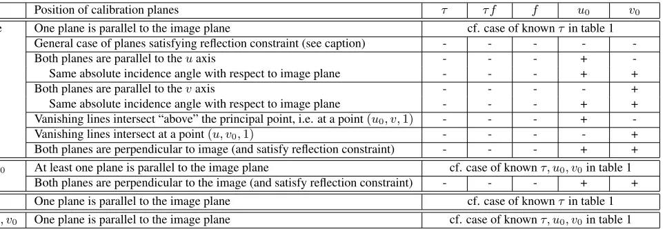
Prior Position of calibration planes τ τ f f u0 v0
None One plane is parallel to the image plane cf. case of knownτin table 1 General case of planes satisfying reflection constraint (see caption) - - - -
-Both planes are parallel to theuaxis - - - +
-Same absolute incidence angle with respect to image plane - - - + +
Both planes are parallel to thevaxis - - - - +
Same absolute incidence angle with respect to image plane - - - + + Vanishing lines intersect “above” the principal point, i.e. at a point(u0, v,1) - - - +
-Vanishing lines intersect at a point(u, v0,1) - - - - +
Both planes are perpendicular to image (and satisfy reflection constraint) - - - + +
u0, v0 At least one plane is parallel to the image plane cf. case of knownτ, u0, v0in table 1
Both planes are perpendicular to the image (and satisfy reflection constraint) - - - + +
τ One plane is parallel to the image plane cf. case of knownτin table 1
τ, u0, v0 One plane is parallel to the image plane cf. case of knownτ, u0, v0in table 1
Table 2: Singularities of calibration from two planes. The cases of parallel planes are not displayed, but may be consulted in the appropriate parts of table 1 on one-plane calibration. In all other configurations not represented here, all intrinsic parameters can be estimated. The “reflection constraint” that is mentioned in three cases, means that the vanishing lines of the two planes are reflections of each other by both a vertical and a horizontal line in the image.
6
Experimental Results
[image:6.612.76.558.461.627.2]6.1
Simulated Experiments
For our simulated experiments, we used a diagonal calibration matrix withf = 1000andτ = 1. Calibration is performed using the projections of the 4 corner points of squares of size 40cm. The distance of the calibration squares to the camera is chosen such that the projections roughly fill the512×512image plane. The projections of the corner points are perturbed by centered Gaussian noise of 0 to 2 pixels variance.
[image:7.612.202.410.221.367.2]In the following, we only display graphs showing the behavior of our algorithm with respect to other parameters than noise; note however that in all cases, the behavior with respect to noise is nearly perfectly linear. The data in the graphs shown stem from experiments with a noise level of 1 pixel. The errors shown in the graphs are absolute errors (the errors for the aspect ratio are scaled by 1000). Each point in a graph represents themedianerror of 1000 calibration experiments. The graphs of the mean errors are very similar, though slightly less smooth.
Figure 1: Scenarios for simulated experiments.
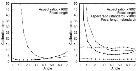
One plane seen in one view. The scenario of the first experiment is depicted in the left part of figure 1. Calibration is performed for different orientations of the square, that range from0◦(parallel to the image plane) to 90◦ (perpendicular to the image plane). The results of calibrating the aspect ratio and the focal length (the principal points is given) are shown in the left-hand part of figure 2. An obvious observation is the presence of singularities: the error of the aspect ratio increases considerably as the calibration square tends to be perpendicular to the image plane (90◦). The determination of the focal length
is impossible for the extreme cases of parallelism and perpendicularity. Note that these observations are all predicted by table 1. In the range of[30◦,70◦], which should cover the majority of practical situations, the relative error for the focal length is below1%, while the aspect ratio is estimated correctly within0.01%.
0 5 10 15 20 25 30 35 40 45 50
0 10 20 30 40 50 60 7
Calibration error
Angle Aspect ratio, x1000
Focal length 0 5 10 15 20 25 30 35 40 45 50
0 10 20 30 40 50 60 7
Calibration error
Angle Aspect ratio, x1000
Focal length Aspect ratio (standard), x1000 Focal length (standard)
[image:7.612.189.424.571.693.2]Two planes seen in one view. In the second scenario (cf. right part of figure 1), calibration is performed with a camera rotating about its optical axis by0◦to90◦. Two calibration planes with an opening angle of90◦ are observed. Plane-based calibration is now done without any prior knowledge of intrinsic parameters. For comparison, we also calibrate the camera with a standard method, using full 3D coordinates of the corner points as input. The results are shown in the right hand part of figure 2.
As expected, the standard calibration approach is virtually insensitive to rotation about the optical axis. As for the plane-based method, the singularities for the estimation of the aspect ratio and the focal length for rotation angles of0◦and90◦are predicted by table 2 (the reflection constraint is satisfied, the planes are parallel to eitheruorv axis and the vanishing lines intersect above or at the same height as the principal point).
As for the intermediate range of orientations, we note that the estimation of the aspect ratio by the plane-based method is 3 to 4 times worse than with the standard approach, although it is still quite accurate. As for the focal length, the plane-based estimate is even slightly better for orientations between30◦and70◦. The error graphs foru0andv0are not shown; for both
methods they are nearly horizontal (which means that there is no singularity), the errors of the plane-based estimation being about30%lower than with the standard approach.
6.2
Calibration Grid
We calibrated a camera from images of a 3D calibration grid with targets arranged in three planes (cf. figure 3). For comparison, calibration was also carried out using a standard method. We report here the results of two different experiments. First, 4 images were taken from different positions, but with fixed calibration. The camera was calibrated from single views in different modes: standard calibration using all points, standard calibration with points from two planes only, plane-based calibration from one, two or three planes with different levels of prior knowledge (cf. table 3). Prior values were taken from the results of standard calibration.
[image:8.612.166.437.425.588.2]Table 3 shows the mean values and standard deviation of the calibration results, computed over the 4 different views used and over all possible combinations of planes. We note that even the one-plane method gives results very close to those of the standard method that uses all available points and their full 3D coordinates. The precision of the plane-based results is lower than for full standard calibration, though comparable to standard calibration using points on two planes. An important observation is that the results are very accurate despite the proximity to singular configurations. This may be attributed to the very high accuracy of the data.
Figure 3: Images of calibration grid and lab scene.
For the second experiment with the calibration grid, we took images at 5 different zoom positions. The camera was calibrated using the5×3 calibration planes simultaneously, where for each view an individual focal length and principal point was estimated. Table 4 shows the results for the focal lengths, compared to the results of standard calibration from the single views at each zoom position. The deviation increases with the focal length, but the errors stay well below the1%mark (if we take the results of standard calibration as ground truth).
6.3
Lab Scene
Method τ f u0 v0
Standard calibration from three planes 1.0284±0.0001 1041.4±0.6 241.6±0.8 325.9±1.8 Standard calibration from two planes 1.0285±0.0002 1042.1±3.3 242.3±3.1 326.2±2.6 One plane,u0, v0known 1.0355±0.0162 1044.5±9.0 241.6±0.7 325.9±1.6
One plane,τ, u0, v0known 1.0284±0.0001 1041.2±3.7 241.6±0.7 325.9±1.6
Two planes, nothing known 1.0303±0.0045 1043.6±4.7 240.7±5.1 325.6±2.4 Two planes,τknown 1.0284±0.0001 1040.7±2.7 240.8±2.2 326.2±1.4 Two planes,u0, v0known 1.0291±0.0019 1040.2±2.5 241.6±0.7 325.9±1.6
Two planes,τ, u0, v0known 1.0284±0.0001 1040.3±2.1 241.6±0.7 325.9±1.6
[image:9.612.105.504.89.202.2]Three planes, nothing known 1.0302±0.0018 1039.9±0.7 239.7±1.6 326.1±0.5
Table 3: Results of calibration using calibration grid.
Method Focal lengths
Standard 714.7 1041.4 1386.8 1767.4 2717.2 Plane-based 709.9 1042.7 1380.2 1782.8 2702.0
Table 4: Calibration results with variable focal length.
distances 1-2, 1-3 and 2-3 were 4mm, 3mm and 0mm respectively, for absolute distances of 275mm, 347mm and 214mm. These results are about as good as we might expect: the edges of the rectangular patch are rounded, thus not reliably extracted in the images. The measured point distances are “extrapolated” from this rectangle, thus amplifying the errors of edge extraction.
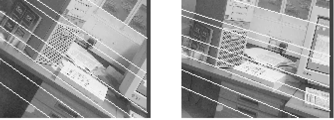
Another result concerns the epipolar geometry of the image pair that was computed from calibration and pose, shown in figure 4. The distance of points to epipolar lines computed from corresponding points in the other image is about 1 pixel, even at the borders of the image.
This simple experiment highlights two important issues. First, besides calibrating the views, we readily obtain their pose in a
[image:9.612.136.472.428.549.2]metric3D frame. Second, we obtain reasonable estimates of matching constraints, potentially for distant views. These aspects are further discussed in the following section.
Figure 4: Computed epipolar geometry for lab scene.
6.4
Distortion Removal
On top of calibrating the intrinsic parameters of the pinhole model, it is in practice often necessary to also calibrate distortion parameters. Figure 5 shows an example, where this was done via a straightforward bundle adjustment type non-linear optimi-sation of all involved parameters (intrinsic parameters, including radial distortion, and the pose of all views), starting from an initialisation with the above described method.
7
Applications
Cheap Calibration Tool. Planar patterns are easy to produce and cheap, while enabling a reasonably reliable calibration.
Reconstruction of Piecewise Planar Objects from Single Views. Using geometrical constraints such as coplanarity, paral-lelism, right angles etc., 3D objects may be reconstructed from a single view (see e.g. [9]). Our calibration method requires knowledge of the metric structure of planes. This requirement may be relaxed by simultaneously determining calibration and plane structure. For example, from a single view of a planar patch that is known to be rectangular, we are able to determine the ratio of the rectangle’s edge lengths as well as the focal length using linear equations. We are currently examining this in combination with coplanarity constraints for the purpose of reconstructing objects from single views. Examples are shown in appendix A.2.
Reconstruction of Indoor Scenes from Many Views. Our calibration method is the central part of ongoing work on a system for interactive multi-view 3D reconstruction of indoor scenes, similar in spirit to the approaches presented in [9, 10]. The main motivation for using plane-based calibration is to make a compromise between requirements on flexibility, user interaction and implementation cost. We achieve flexibility by not requiring off-line calibration: our calibration patterns, planar objects, are omnipresent in indoor scenes. The amount of user interactions is rather little: we usually use rectangles as calibration objects; they have to be delineated in images and their edge lengths measured (this might also be avoided as indicated above). By identifying planar patterns across distant views, we not only can simultaneously calibrate many views but also compute a global initial pose of many views to bootstrap wide baseline matching for example. The pose and calibration of intermediate views can be “interpolated” from neighboring already calibrated views using local structure from motion techniques. This scheme relies on methods that are relatively simple to implement and might provide a useful alternative to completely automatic techniques such as [8] that are more flexible but more difficult to realise.
Augmented Reality. A nice and useful application of plane-based calibration and pose determination is presented in [5]. Rectangular plates are used to mark the position and orientation of non planar objects to be added to a video sequence, which is in some way a generalisation of “overpainting” planar surfaces in videos by homography projection of a desired pattern. Plane-based methods may also be used for blue screening; attaching calibration patterns on the blue screen allows to track camera pose and calibration and thus to provide input for positioning objects in augmented reality.
8
Conclusion and Perspectives
We presented a general and easy to implement plane-based calibration method that is suitable for calibrating variable intrinsic parameters and that copes with any number of calibration planes and views. Experimental results are very satisfactory. For the basic cases of using one or two planes, we gave an exhaustive list of singularities, thus allowing to avoid them deliberately and obtain reliable results. Several applications of plane-based calibration were described.
Ongoing work is mainly focused on the completion of an interactive system for 3D reconstruction of indoor scenes from many images, that is mainly based on our calibration method. An analytical error analysis might be fruitful, i.e. examining the influence of feature extraction errors on calibration accuracy.
References
[1] A. Criminisi, I. Reid, A. Zisserman, “Duality, Rigidity and Planar Parallax,”ECCV, pp. 846-861, June 1998.
[2] O. Faugeras, “Stratification of Three-Dimensional Vision: Projective, Affine and Metric Representations,”Journal of the Optical Society of America A, Vol. 12, pp. 465-484, 1995.
[3] R.J. Holt, A.N. Netravali, “Camera Calibration Problem: Some New Results,”CVIU, Vol. 54, No. 3, pp. 368-383, 1991.
[4] A. Jennings, J.J. McKeown,Matrix Computation,2nd edition, Wiley, 1992.
[5] M. Jethwa, A. Zisserman, A. Fitzgibbon, “Real-time Panoramic Mosaics and Augmented Reality,”BMVC, pp. 852-862, September 1998.
[6] R.K. Lenz, R.Y. Tsai, “Techniques for Calibration of the Scale Factor and Image Center for High Accuracy 3-D Machine Vision Metrology,”PAMI, Vol. 10, No. 5, pp. 713-720, 1988.
[7] F. Pedersini, A. Sarti, S. Tubaro, “Multi-Camera Acquisitions for High-Accuracy 3D Reconstruction,”SMILE Workshop, Freiburg, Germany, pp. 124-138, June 1998.
[9] H.-Y. Shum, R. Szeliski, S. Baker, M. Han, P. Anandan, “Interactive 3D Modeling from Multiple Images Using Scene Regularities,”SMILE Workshop, Freiburg, Germany, pp. 236-252, June 1998.
[10] R. Szeliski, P.H.S. Torr, “Geometrically Constrained Structure from Motion: Points on Planes,” SMILE Workshop, Freiburg, Germany, pp. 171-186, June 1998.
[11] R.Y. Tsai, “A Versatile Camera Calibration Technique for High-Accuracy 3D Machine Vision Metrology Using Off-the-Shelf TV Cameras and Lenses,”IEEEJournal of Robotics and Automation, Vol. 3, No. 4, pp. 323-344, 1987.
[12] B. Triggs, “Autocalibration from planar scenes,”ECCV, pp. 89-105, June 1998.
[13] G.-Q. Wei, S.D. Ma, “A Complete Two-Plane Camera Calibration Method and Experimental Comparisons,”ICCV, pp. 439-446, 1993.
A
Examples
A.1
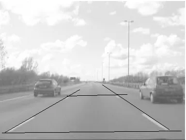
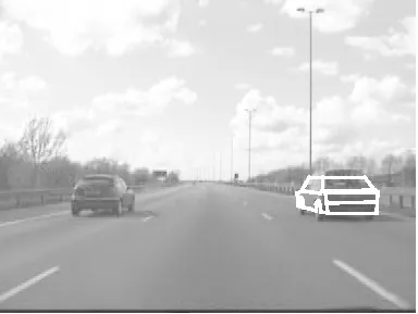
Vehicle Detection
Figure 6: Road markers used for ground plane calibration.
[image:13.612.112.497.420.709.2]A.2
Reconstruction of Piecewise Planar Objects from Single Views
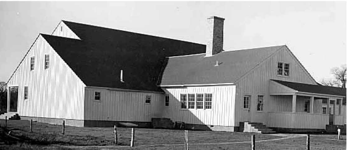
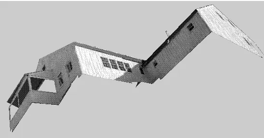
The images in figures 9 and 14 have been used to calibrate the focal length of the cameras and obtain 3D models of the buildings shown. Texture has been mapped from the original images onto the 3D models. Rendered views of the models are shown in figures 10 to 18. Note that for the second building, the original image in figure 14 does not give sufficient texture information for some walls. In this case, for better visualization, we added texture maps from additional close-up views.
[image:15.612.53.611.185.426.2]Input needed for calibration and 3D reconstruction are coplanarity, perpendicularity and parallelism constraints. The com-plete method will soon be described in a separate article.
Figure 10: Sample view of the 3D model.
[image:16.612.52.598.406.692.2]