An Analysis of Dynamic Response of a Rocket Sled

2017 2nd _{International Conference on Artificial Intelligence and Engineering Applications (AIEA 2017)}

ISBN: 978-1-60595-485-1

An Analysis of Dynamic Response of a Rocket Sled

JUN LIU, HUA ZHAO, KAIXUAN GU and WEIHUA WANG

ABSTRACT

The prediction of dynamic response of the rocket sled before the detailed design process would be beneficial as it can help optimize the structure, thereby increasing the reliability, shortening the development cycle, and reducing the risk of developing. However, it is very difficult to accurately simulate the dynamic response of a rocket sled considering the additional elastic deformation and the irregularity of the track surface. A calculation of the difference between the value of track-sled gap and the irregularity of the track surface for estimating elastic deformation can improve the simulation accuracy, but this method does not apply to lower speed, as the impact speed would not cause the same amount of additional deformation calculated. In light of this, an appropriate interpolation method is developed to determine the additional elastic deformation value in lower speed. The results of dynamic response are provided comparing with real test data and it proves that this method is very effective.

KEYWORDS

Dynamic, Rocket sled, Simulation, Elastic deformation.

INTRODUCTION

In the modern high technique condition, many new concepts, new theories, new techniques and new materials are widely applied in all kinds of weapon systems. In order to obtain the dynamic performance of those newly developed weapons, rocket sleds [1-4] are often used to provide a ground test simulating real fly condition. As the name implies, rocket sleds are propelled by one or several engines, flying among special made high precision tracks. Comparing to flight tests and common indoor experiments, the rocket sleds possess the advantage of easy controlled payload ability, running speed, acceleration and environment, and it is convenient for observation and collecting test data repeatedly. As the sled flies along the track, it is in a complex environment including engine thrust, strong impact, aerodynamic drag force etc., resulting in complicated dynamic test environment for the test component. The dynamic performance of the sleds is highly connected with the accuracy of test results and reliability.

The track irregularity and the impact between sled and track are the two most important reasons that cause severe vibration. However, it is very difficult to simulate the operating conditions in the computer using numerical analysis method and the task will be time consuming and computationally expensive, given that the iteration would

_________________________________________

be huge for calculating the contact deformation caused by irregularity. Therefore it is not much of practical value to simulate the whole system in the design progress. In order to secure the safety of the test, traditionally the designers tend to choose a large

Safety factor when designing the structure. But this has led to the cumbersome sled body, resulting in not only the increase of engine number and high cost of the test, but also less stabilization and a limitation of pushing speed boundaries. In light of this fact, instead of running massive iterations to obtain the additional contact force caused by the irregularity of the track, this paper uses a computationally cost-effective approach - elastic deformation revise method to complete the simulation task. This paper applies finite element analysis (ANSYS) [5, 6] together with interpolation method to simulate the flight of a rocket sled. The dynamic simulation research of the sled-track coupling system can effectively estimate the actual dynamic response of the flying rocket sled, providing a reference for designing the rocket sleds, and thereby help optimizing the design and increase reliability.

ASSUMPTIONS

This study is based on assumptions below.

The track irregularity is rigid, namely the elastic deformation caused by irregularity is not considered during analysis.

The track and sled are considered to be elastic material.

The vibration effect on the track caused by irregularity is much more serious than on the sled.

PROCEDURE OF ANALYSIS

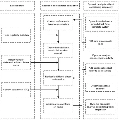
The dynamic response analysis contains four steps. The first is to establish the finite element model (FEM) of the track without the irregularity data and implement the transient analysis. The second step is to extract the dynamic parameters on the contact node, including the track-sled gap, vertical relative speed, forward relative speed and the irregularity value of the node. The third step is to calculate the additional elastic deformation caused by track irregularity using the parameters extracted, and thereby calculate the additional vertical contact force. The last step is to apply the additional contact force on the contact node, together with thrust, gravity and aerodynamic drag, and then conduct the transient analysis again. Thus, the dynamic response of the rocket sled is yielded considering the track surface irregularity. The progress of finite simulation analysis is illustrated in Figure 1.

2.1 The Extraction of Transient Parameter of a Node

Typical locations of contact nodes can be seen in Figure 2. The additional contact force caused by track irregularity can be obtained by extracted dynamic parameter and calculation, as shown in Figure 3.

2.2 Calculation of the Additional Contact Deformation

Considering the computational time and resource, it is not wise to go through,

Figure 1. Finite Analysis procedure of the rocket sled.

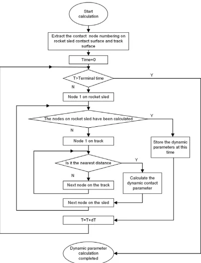
Figure 3. The flow chart of dynamic parameters extraction.

Iteration process to obtain the additional contact deformation. An evaluation of deformation is conducted through analysis below.

Vx Slipper

Theoretical gap Base level on the track surface Track irregularity

Theoretical additional elastic deformation

Figure 4. Theoretical additional elastic deformations.

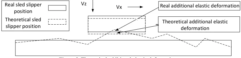
Vz Theoretical additional elastic  deformation Vx Real sled slipper  position Theoretical sled  slipper position Real additional elastic deformation

Figure 5. Theoretical additional elastic deformations.  

However, the impact effect is not considered in this conception. In low speed, because of the very low vertical impact speed, the impact effect between the sled and track is small. Therefore, the theoretical additional deformation is bigger than the real value, as shown in Figure 5.

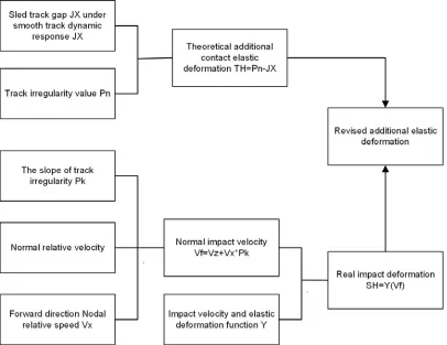
An interpolation method is used to obtain the additional elastic deformation, as shown in Figure 6. Firstly the relation curve of the impact velocity and deformation was established. Then the theoretical additional contact elastic deformation was obtained through comparison of sled-track gap value and track irregularity value. Next, the impact velocity is calculated according to the track irregularity slope, vertical relative speed hand forward speed of the node, and thereby the real impact deformation was yielded according to the impact velocity- deformation curve. Finally, the value of real impact deformation was compared with theoretical deformation. If the real impact deformation is less than the theoretical deformation, it means that the impact speed is not enough to trigger the theoretical deformation, and thus the revised deformation value equals to the real impact deformation. If the real impact deformation is more than the theoretical deformation, it implies that theoretical additional elastic deformation happens and thus the revised deformation value equals to the theoretical additional elastic deformation.

2.3 Calculation of the Additional Contact Force

After the revised additional elastic deformation is calculated, the contact force on each node can be calculated using equation of motion.

Figure 6. Revised additional elastic deformation calculation procedure.  

Only the contact force caused by elastic deformation is under consideration here, therefore the force can be calculated as equation 1.

n

F    k  c  (2)

Where k is the impact contact stiffness, and c is the impact contact damping. k=2.283e5 N/mm

The contact forces are added on every node on the contact surfaces. The values depend on the additional elastic deformation and the additional elastic impact velocity. There are 60 nodes even distributed on the contact surfaces, and the contact stiffness and damping of every node are simplified as 1/60 of that of the whole sled system.

2.4 The interpolation curve of Impact velocity and deformation

Figure 7. Finite element model of the Sled-track system.

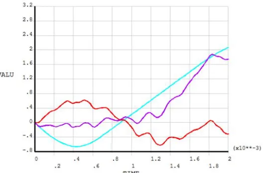
Figure 8. Vertical impact responses of velocity = 50 mm/s.  

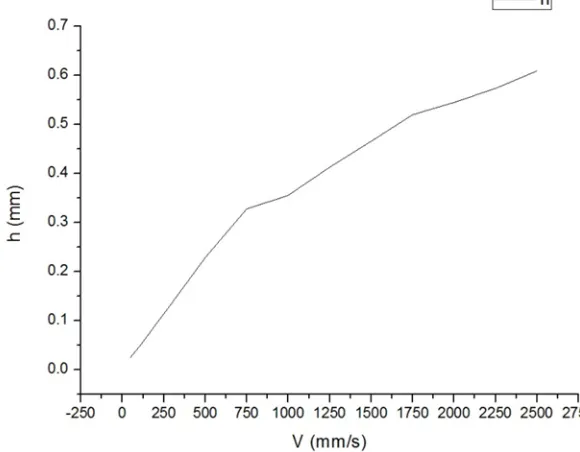
Figure 10. Deformation with regard to velocity.

(a) (b) Figure 11. Geometry model and finite element model.

(a. Geometry model b. Finite element model)

Of averaged displacement of the top and bottom surface was considered to be equivalent as impact stroke.

It can be seen from these figures that the elastic deformation increases as the speed increases. The impact deformation curve, namely the interpolation curve of Impact velocity and deformation, can be plotted according to impact deformation value in different speeds, as shown in Figure 10.

DYNAMIC ANSLYSIS OF ROCKET-SLED SYSTEM USING FINITE ELEMENT MODEL

Geometry and Material Properties

TABLE 1. MATERIAL PROPERTIES.

Steel(Track) Steel(Track) Steel(Track)

Elasticity modulus 2.0E5 2.0E5 2.0E5

Poisson’s ratio 0.3 0.3 0.3

Density(t/mm3_{) 7.85E-9 7.85E-9 7.85E-9}

Loads and Working Conditions

THE THRUST OF THE ROCKET ENGINE

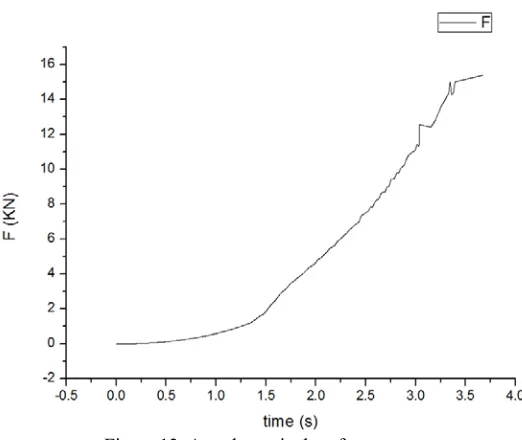
This study analyzes initial 500m of the accelerating section, namely the initial 2s of engine thrust in the time history. However, the mass needs to be corrected considering the burning loss. As the burning rate is a constant, the engine thrust can be corrected such that with a constant mass, the heading acceleration is the same as that of a varying mass with a constant burning rate. The corrected engine thrust curve is shown in Figure 12. The correcting formulas used are shown in the following expression:

( ) ( )

( )

r

DX

F t M M k t a

F t M a

   

 

Where F (t) is the thrust, M is the total mass except the fuel, Mr. is the fuel mass, k is the fuel consumption rate, and FDX (t) is the corrected engine thrust.

THE CALCULATION OF WIND LOAD

The wind load was calculated through CFD simulation in regard to velocities of test data. The total wind load was simplified as distributed to resistance surfaces. Thus the aerodynamic drag force curve can be obtained shown in Figure 13.

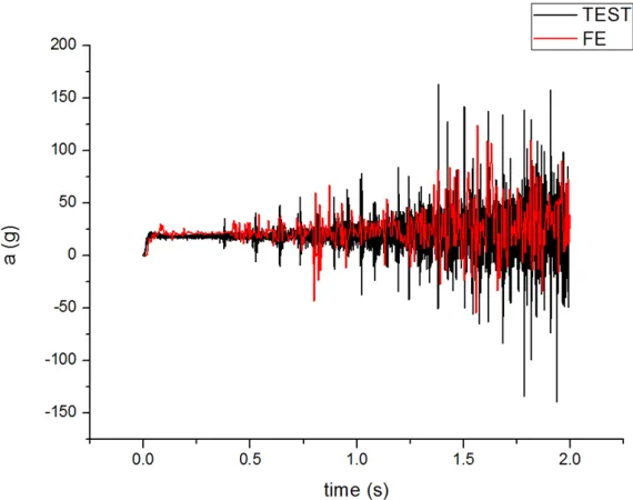
SOME RESULTS OF DYNAMIC RESPONSE COMPARED WITH TEST DATA

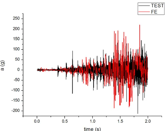
Using the analysis procedure mentioned in section 2, a simulation was completed for 500m acceleration stage of rocket sled operation. The simulation time is 2 seconds. The observation location of the output parameter is between the second and the third slippers. The vertical, lateral, and heading accelerations of the test and simulation are shown in Figure 14, 15, 16 respectively.

DISCUSSION

Figure 12. Time history of corrected engine thrust.

Figure 13. Aerodynamic drag force curve.

When the additional contact force was not added, the sled glides smoothly without Lateral and vertical acceleration. When the sled gradually encounters irregularities, progressive vibration gradually occurs. It can be inferred that the vertical and lateral acceleration are caused by irregularity of the track.

CONCLUSION

Figure 14. Vertical acceleration in contrast with test data.

Figure 16. Course acceleration in contrast with test data.

Dynamic loads, enabling structure optimization and reducing the safe risk. It can be seen from the results that there is no large difference between test data and the virtual simulation. Particularly in low speed, the good agreement of the test and virtual simulation proves that the elastic deformation revise method has a high accuracy.

REFERENCES

1. Cinnamon J.D., Palazotto A.N. 2009 International Journal of Impact Engineering 36 254-62. 2. Tachau R.D.M., Yew C.H., Trucano T.G. 1995 International Journal of Impact Engineering 17

825-36.

3. Szmerekovsky A.G., Palazotto A.N., Baker W.P. 2006 International Journal of Impact Engineering 32 928-46.

4. Laird D.J. , Palazotto A N 2004 International Journal of Impact Engineering 30 205-23. 5. Gerstle Jr. F.P., Follansbee P.S., Pearsall G.W., Shepard M 1973 Wear 24 97-106. 6. Graff K.F., Dettloff B.B. 1969 Wear 14 87-97.