Review on Design and Implementation of Audio Signal Classification System to classify the Media in Speech/Music

(1)

Review on Design and Implementation of

Audio Signal Classification System to classify

the Media in Speech/Music

Prof.P.B.Vikhe

1,

_{Bhutkar Aparna}

2

_{, Khandare Archana}

3

_{, Mahale Vaishali}

4

1

_{Asst.Prof., Computer Engineering, P.R.E.C, Maharashtra, India}

234

_{Student, Computer Engineering, P.R.E.C, Maharashtra, India}

ABSTRACT

Over the last few years exceeding efforts have been made to develop methods for extracting information from audio-visual media, mandate that they may be stored and retrieved in databases automatically. Audio classification serves as the fundamental step towards the quickly growth in audio data volume. Automatic audio classification is very useful in content based audio retrieval and online audio distribution. The accuracy of the classification relies on the efficacy of the features and classification scheme. In this work both, time domain and frequency domain features are extracted from the input signal. Time domain feature is Root Mean Square (RMS). Frequency domain feature is spectral flux. After feature extraction, classification will be. The selection of the important features is explained as well as the classifiers used for classification are compared.

Key Words: (Size 10 & Bold) Key word1, Key word2, Key word3, etc (Minimum 5 to 8 key words)…

1. INTRODUCTION

Classification can feed useful information for grasping and analysis of audio content. It is of critical importance in audio indexing. Feature analysis and extraction are foundation steps for audio classification and identification. All classification systems engage the cognition of a set of features from the input signal. Each of these emblems represents an element of the emblem. In many applications there is a virile interest in segmenting and classifying audio signals. A first accessories characterization could be the digest of an audio signal as one of speech, music. Audio vector in the feature space. The dimension of the feature space is equality to the number of extracted features. These features are given to a Classifier that employs some rules to assign a class to the incoming vector. Fig shows the block diagram, which is self-explanatory. [2]

Fig -1: block diagram

2. FEATURE SELECTION

(2)

© 2016, IRJET ISO 9001:2008 Certified Journal Page 1336 1) Invariance to irrelevancies: Any good feature should exhibit invariance to irrelevancies such as noise, bandwidth or the exuberance scaling of the signal. It is also upon the classification system to consider such contrast as irrelevant to accomplish better classification across a wide range of audio formats.

2) Discriminative Power: The motive of feature selection is to achieve discrimination among distinct classes of audio patterns. Therefore a feature must take round about similar expense within the same class but distinct values across different classes.

3) Uncorrelated to other features: It is very influential that there are no redundancies in the emblem space. Each new feature that is selected must give altogether distinct information about the signal as possible. This useful in better computation capability, improved performance and optimization of value.

Considering all above points we have selected following features:

1.3 Root Mean Square (RMS) [1]

For a short audio signal (frame) consisting of N samples, the amplitude of the signal measured by the Root Mean Square is described by equation. RMS is a measure of the loudness of an audio signal and since changes in loudness are important cues for new sound events it can be used in audio segmentation. In this project the distribution of the RMS features are used to detect boundaries between speech and music signals. The method for detecting boundaries is based on the dissimilarity measure of these amplitude distributions.

A= (1)

1.2 Spectral Flux (SF)[4][6]

Spectrum flux (SF) is defined as the average variation expenses of spectrum between two coherent frames in a given clip. In general, speech signals are tranquil of changing voiced sounds and unvoiced sounds in the syllable proportion, while music signals do not have this kind of architecture. Hence, for speech signal, its spectrum fluxion will be in general greater than that of music. Spectrum flux is a good feature to discriminate among speech and music.

(2)

1.3 Classification.

i).KNN [3]

The k-nearest neighbor algorithm (k-NN) is a never-parametric method for classifying objects based on nearest training examples in the feature space. An object is grouped by a majority vote of its neighbors, with the object being constituted to the class most simple amongst its k nearest neighbors (k is a positive integer, typically small). If k = 1, then the object is simply constitute to the class of its nearest neighbor .The educational examples are vectors in a multidimensional ensign space, each with a class label either s p (speech) or mu (music). The training phase of the algorithm constraint only of storing the ensign vectors and class labels of the training samples. Each tuples represents a point in an n-dimensional pattern space, i.e. here 5-dimensional.

Closeness is called in terms of a distance metric, such as Euclidean distance.[5]The Euclidean distance during two points or tuples X=(x1,x2,…. xn) and Y=(Y1,Y2...Yn) is for each numeric attribute ,we take difference between the corresponding values of that attribute in tuple X and in tuple Y, square this difference and grow it. The square root is taken of the total accumulated distance count. Typically, we normalize the values of each ton before using distance equation. This helps prevent attributes with initially huge ranges from outweighing attributes with initially smaller ranges. Formula for Normalization,

Normalization= (4)

(3)

ii) Bayesian Classifier [3]

Naive Bays classifier is simple possibilities classifier depend on inure Bays theorem with strong (naive) independence predictions.

The naive Bayesian classiﬁer concern as follows:

1. Let T be a educational set of samples, each with their class labels (speech C1 or music C2). Each sample is represented by an n-dimensional vector, X = {x1, x2, . . . , xn}, describing n measured expenses of the n attributes, A1, A2, . . . , An, respectively.

2. Given a sample X, the classiﬁer will assume that X belongs to the class having the highest a posteriori probability, conditioned on X. That is X is assumed to belong to the class C1 if and only if

P(C1|X) > P(C2|X) .Thus we ﬁnd the class that maximizes posteriori probability.

By Bays’ theorem (prameyas)

P(Ci|X) = P(X|Ci) P(Ci)/P(X)

3. As P(X) is the same for all classes, only

P(X|Ci) P(Ci)

require to be maximized. These classes are equally likely, that is, priori probabilities

P (C1) = P(C2) and we would therefore maximization P(X|Ci).

4. Given data sets with so much attributes, it would be computationally expensive to compute P(X|Ci) . In order to curtail computation in evaluating

P(X|Ci) P(Ci) , the naive predictions of class conditional independence is made. This consider that the values of the attributes are qualified independent of one another, as per given the class label of the sample. Mathematically this means that

(5)

If Ak is continuous-valued, then we typically assume that the values have a Gaussian allocation with a mean µ and standard deviation σ deﬁned by

(6)

so that p(xk|Ci) = g(xk, µCi , σCi ).

We require to enumetate µCi and σCi , which are the mean and standard deflect of expenses of ton Ak for training samples of class Ci.

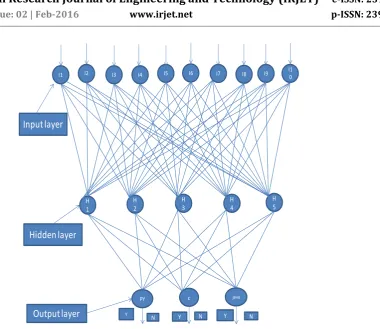
5. In order to assume the class label of X, P(X|Ci) P(Ci) is calculated for each class Ci . The classiﬁer predicts that the class label of X is Ci according to the posteriori probability. iii).ANN by using Back propagation algorithm

(4)

I1 I2 I3 I4 I5 I6 I7 I8 I9 I1₀

H 4 H

3 H

2 H

1

H 5

java c

PY

Input layer

Hidden layer

Output layer

Y

N Y N Y N

Fig -2: Back Propagation network example

The network is first starting by setting up all its significance to be small random numbers say between –1 and +1. Next, the input sample is applied and the out -tum calculated .The calculation gives an output which is completely distinct to what you want, since all the significance are random. We then calculate the fault of each neuron, which is calculated by Target - Actual out tum. This fault is then antiquated mathematically to change the significance in such a way that the fault will get smaller. In other words, the Outcome of each neuron will be get closer to its Target. In each iteration we are analyzing the out tum value of each sample in training data by considering its class and according to that we have to set the threshold value for testing purpose which will classify the input sample. The architecture of back propagation algorithm is as above.

A) Neural Network Model

A neural network model is a powerful tool used to perform ideal recognition and other intelligent tasks as performed by human brain. The neural network request for ideal recognition is depend on the type of the learning mechanism applied to induce the out tum from the network. The learning classified or categorized one as a supervised leaning in which the desired response is known to the system i.e. the disposal is trained with the prior data available to obtain the desired out tum. In case of this type of learning, if the computed out tum does not match the desired out tum, then the difference between the two is appoint which is eventually antiquated to change the external parameters required to produce the correct out tum.

The most common supervised neural network example is Multi-layer Perceptron If the network is based on the unsupervised learning, and then the out tum is produced based on prior assumptions and observations however, the desired reaction is not known. Kohonen Self-organizing scheme /Topology-preserving scheme network is based on unsupervised apprehend low. The another third type of apprehend is reinforcement apprehend wherein the carry of the network is predicted depends on the feed-back from the retro surrounding which also forms a part of neural network design request however supervised and unsupervised apprehend rules are more commonly precede for implementation of the network design.

[image:4.595.139.520.57.386.2]

(5)

B) Implementation of Back-Propagation Algoritham.

The Multi-layer association using the back-propagation algorithm:

i. The network basically includes of three layers: input flake, out tum flake and the middle layer i.e. the hidden flake.

ii. These layers consist of the neurons which are connected to form the entire network.

iii. Significance is assigned on the connections which marks the signal strength. The significance cost is calculated based on the input signal and the fault function back propagated to the input flake.

iv. The role of hidden layer is to update the significance on the connections based on the input signal and fault signal. Lowed immediately by the significance update or batch mode in which the significance updating take place after many propagation. Usually batch mode is followed due to minimum time consume and less no. of propagate iterations.

viii. The advantage of using this algorithm is that it is simple and easy to use also well suited to provide a solution to all the complicated patterns.

ix. The implementation of this algorithm is useful and also faster depending upon the amount of input-out tum data available in the flake.

C) Applications for Neural Networks.

Neural Networks are successfully being antiquated in many areas often in brace with the use of Other AI techniques-

1) A classic neural network is used for image recognition. A network that can classify diverse standard images can be usage in several areas.

2) Quality assurance, by classifying a metal welding as whether is contains the property standard.

3) Medical diagnostics, by classifying x-ray image for tumor diagnosis.

4) Detective tools, by classifying fingerprints to a database of suspects.

5) A well-known impersonation using image recognition techniques is the Optical Character Recognition .tools that we find accessible with the standard scanning software for the home computer. Scan-soft has had great victory in combining NN with a rule based system for correctly endorsing both characters and words, to get a high level of accuracy 1.

3. TRAINING TESTING VALUATION

3.1 Test information

Another set of information was used to determine the accuracy of the proposed features and categorization system. This set of test information consisted of 25 samples each of music and speech. Each sample was between 4 and 5 seconds long, in order to keep it similar to the train data. The music samples were obtained from major personal accumulations and attempts were made to consist all types of instrumental music. For speech samples attempt were made to consist both male and female speakers and pattern with both single and multiple voices.

3.2 Evaluation of classifiers:

After the detection of features in the audio taxonomy and its subsequent class detection it is also important to evaluate the accuracy of the output, that is the final class of the audio. This evaluation also gives an idea about the performance of the system, which in turn gives the detail about the efficiency of the different algorithms. This narrows down to one aspect i.e. the performance of the classification used. This is normally evaluated using the confusion matrix.

(6)

an instance is speech, b is the number of incorrect assumptions that an instance is music, c is the number of incorrect of assumptions that an instance speech, and d is the number of correct.

Predictions that an instance is music. Therefore the confusion matrix can be constructed as follows:[2]

Predicted

Speech Music

Actual Speech A B

Music C D

Therefore the classification matrix gives a general idea as to how the classification has Performed. It is also important to note the efficiency of the confusion matrix. The most Important property that describes this efficiency is the accuracy of the confusion matrix. The accuracy is the proportion of the total number of assumptions that were correct. It can be defined by the equation

(a + d) / (a +b +c + d)

Result:

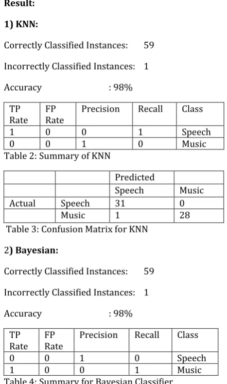
1) KNN:

Correctly Classified Instances: 59

Incorrectly Classified Instances: 1

Accuracy : 98%

TP

Rate FP Rate Precision Recall Class

1 0 0 1 Speech

[image:6.595.32.266.356.752.2]

0 0 1 0 Music

Table 2: Summary of KNN

Predicted

Speech Music

Actual Speech 31 0

Music 1 28

Table 3: Confusion Matrix for KNN

2) Bayesian:

Accuracy : 98%

TP

0 0 1 0 Speech

1 0 0 1 Music

Table 4: Summary for Bayesian Classifier

Classifier Accuracy (in %)

KNN 98

Naïve Bays’ 98

(7)

Speech Music

Actual Speech 30 1

Music 0 29

Table 5: Confusion Matrix for Bayesian Classifier

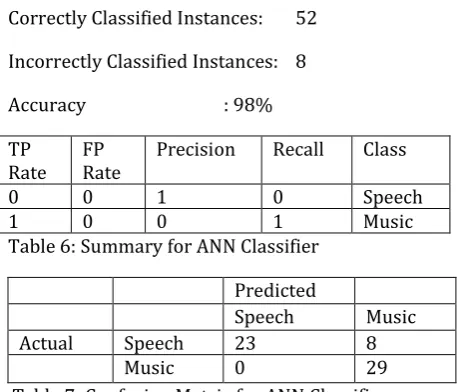
3) ANN

Accuracy : 98%

TP

0 0 1 0 Speech

[image:7.595.32.261.194.390.2]

1 0 0 1 Music

Table 6: Summary for ANN Classifier

Predicted

Speech Music

Actual Speech 23 8

Music 0 29

Table 7: Confusion Matrix for ANN Classifier

From this confusion matrix we can predict accuracy of classifier.

Table 8: Accuracy of classifiers given below.

5. Graphical representation for accuracy of three classifiers

KNN (98%) Bayesian (98%) ANN (86%)

Graph 2: Accuracy of three classifiers

CONCLUSIONS

We have done classification using three classifiers: K-nearest neighbor, Naïve Bays’ classifier and ANN using back-propagation algorithm. Out of these three classifiers KNN and Naïve Bayesian has accuracy above 90% .We have also done separation of single folder of all audio files into two separate folders as speech and music based on class which is given as output by the classifier.

REFERENCES

1. Abdullah Hussein Omar ‘Audio Segmentation and Classification’ February 28, 2005 2. Hariharan Subramanian ‘AUDIO SIGNAL CLASSIFICATION’ November2004 3. Jiawei Han and MichelinKamber‘Data Mining Concepts and techniques’

4. R. Thiruvengatanadhan, P. Dhanalakshmi, P. Suresh Kumar speech/Music Classification Using SVM’ March 2013

5. Charles Elkan‘Nearest Neighbor Classification’ January 11, 2011