ANN Methods for COP Prediction of Supermarket Refrigeration System

2019 International Conference on Artificial Intelligence, Control and Automation Engineering (AICAE 2019) ISBN: 978-1-60595-643-5

ANN Methods for COP Prediction of Supermarket Refrigeration System

Wei-le OUYANG and Rui-qing KANG

School of Automation and Electrical Engineering, University of Science and Technology Beijing, Beijing, China

*Corresponding author

Keywords: BP neural network, Genetic algorithm, RBF neural network, COP prediction, Refrigeration system.

Abstract. Refrigeration system is one of the main energy consumers. Since COP prediction is the base of optimization analysis of energy saving, ANN models were developed by using on-site testing data to predict COP of the refrigeration system in this paper. BP and RBF neural network were applied to the prediction models respectively, and genetic algorithm was used to optimize the BP network. The prediction results of the models show that the GA-BP model has higher accuracy and better stability than the BP network only. And the RBF model has the smallest error and shortest time on calculation. Both BP and RBF models can apply in COP prediction of the refrigeration systems, but performance of the RBF model is better.

Introduction

Energy saving and emission reduction are significant missions for Chinese government. Refrigeration units for selling and storing foods is one of the main energy consumers in supermarkets. COP for a refrigeration system is defined as the ratio of the cooling capacity output to the total electric power input. It is used to show the efficiency of the entire system. Workers in the supermarket usually adjust parameters manually to improve efficiency based on experience. In order to use intelligent control system, COP prediction is need to be done before the optimization analysis of energy saving. How to build an accurate COP prediction model is a primary issue for saving energy.

ANN methods provide new solutions for complex nonlinear problems to predict the performance of refrigeration system. Tian et al. put forward a BP neural network to predict the COP of a variable frequency screw chiller in a cinema, which achieved high accuracy [1]. Xue et al. compared different black-box prediction models and found out BP is the proper model in predicting COP of chiller accurately. And by adopting GA-based operating variables identification, optimal values of the variables were found in specified ranges as well[2]. Lazrak et al. also developed an ANN approach to evaluate the energy performance of absorption chillers, but the reliable information with the long-term performance of the systems was obtained from a laboratory [3]. Arzu et al. used ANNs for performance analysis of a single-stage vapor compression refrigeration system. And mathematical formulations had been obtained from the summation and activation functions and weights of neurons [4]. However, most of researches fixed on air conditioners or a single unit, few studies are on a whole system. Additionally, most of studies used experimental data to simulate systems. In this paper, different ANN models were proposed to predict COP of the refrigeration system in a supermarket. And all data we used were on-site testing data, which showed different conditions from the performance shown in laboratory. This would provide more theoretical basis for optimizing energy-saving control system.

Data Preparation

COP of the system as the output of the ANN models, this paper used software REFLIBfxl. With the help of this tool thermodynamic data and transport properties of refrigerants can be calculated within EXCEL simply. Although REFLIBfxl can calculate the COP instead of complex thermodynamic equations, it cannot be applied to the real-time intelligent control system, so machine learning is applied to predict the COP.

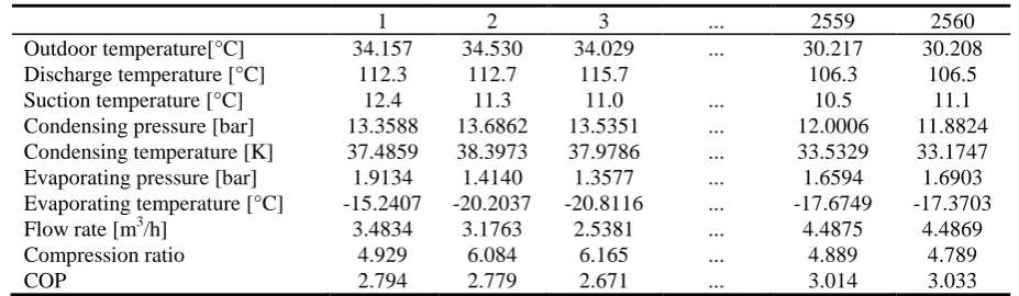
Table 1. Part of operating data samples.

1 2 3 ... 2559 2560

Outdoor temperature[°C] 34.157 34.530 34.029 ... 30.217 30.208

Discharge temperature [°C] 112.3 112.7 115.7 106.3 106.5

Suction temperature [°C] 12.4 11.3 11.0 ... 10.5 11.1

Condensing pressure [bar] 13.3588 13.6862 13.5351 ... 12.0006 11.8824 Condensing temperature [K] 37.4859 38.3973 37.9786 ... 33.5329 33.1747 Evaporating pressure [bar] 1.9134 1.4140 1.3577 ... 1.6594 1.6903 Evaporating temperature [°C] -15.2407 -20.2037 -20.8116 ... -17.6749 -17.3703

Flow rate [m3/h] 3.4834 3.1763 2.5381 ... 4.4875 4.4869

Compression ratio 4.929 6.084 6.165 ... 4.889 4.789

COP 2.794 2.779 2.671 ... 3.014 3.033

Based on the physical laws and theoretical calculation of COP, this paper presents correlation analysis of all variables from Table 1 to determine the input variables of ANN models. We found that all variables are related to COP, while the outdoor temperature, discharge temperature, condensing pressure are significantly related to COP. Since the evaporating pressure and temperature are highly correlated, the condensing pressure and temperature are highly correlated as well, temperatures were omitted in order to make the model more concise. Hence, seven variables of the rest in Table 1 were selected as the input of the ANN models eventually.

Data Preprocessing. On-site measurement data always come with uncertainties that bring about lower accuracy and long training time when a model is developed.Except for purchases, big change in weather or any other uncertain factors, the data should fluctuate within a small range. In this paper, the 3σ rule was adopted. Besides, the actual COP should be less than ideal COP. Ideal value ε for each point were calculated by Eq. 1, and points where the actual COP is bigger than the ideal value should be eliminated. Finally, 36 outliers of original data were eliminated, and the percentage was 1.4%.

e c e T T T    273

 (1)

Where Te is evaporating temperature [°C], Tc is condensing temperature [°C].

Due to the different units and ranges of input variables, the neural network may converge slowly and results may be wrong. Therefore, the original data need to be normalized before network trainning and the output of network should be anti-normalized before analysis.

COP Prediction

The total number of measurement points after preprocessing is 2560 (see Table 1), the first 2510 points are selected for neural network training, and the last 50 are used for testing.

BP Network Model. BP (Back Propagation) neural network is composed of three layers: input layer, hidden layer and output layer. It optimizes the weighted connections by allowing error to spread from output layer towards lower layers. BP models need to determine the number of hidden layer nodes before training. In this paper, we used Eq. 2 to obtain a range for hidden layer nodes l.

a m n

l    (2)

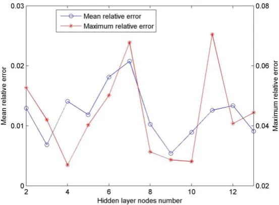
smaller than that at l=3, considering the problem of learning time and over-fitting, the best number of the hidden layer nodes was chosen to be 3 in this paper. Therefore, we can finally determine the BP network structure (see Fig. 2). Log-sigmoid as the hidden layer transfer function f(x) was used. The max iteration number was set to 1000, the network learning rate was 0.01, and the training goal error was 0.001.

Figure 1. Prediction error with different nodes number.

Figure 2. BP neural network structure.

There are two criteria for the network performance, mean relative error (MRE) and coefficient of determination (R2). They defined as Eq. 3 and Eq. 4, respectively.

ˆ 1 M RE 1



Where N is the number of testing samples, yˆi is predicted value of i set, yi is actual value of i set,

andyis the mean value of testing points. The smaller the MRE is and the closer the R2 is to 1, the better performance the model achieves.

network by determining the optimal initial weights and thresholds before training, so that the predicted results will not affected by the initialization of parameters.

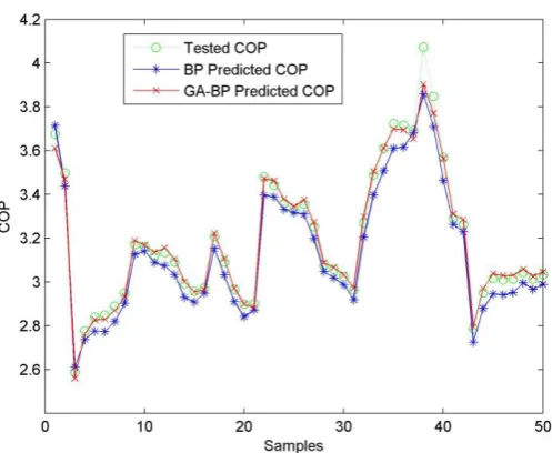
Figure 3. Prediction result of BP model.

GA-BP Model. Genetic algorithm is a method to search for optimal solutions by simulating natural evolutionary processes. The training starts with GA, which performs a global search on weight ranges and find out the best initial weights for BP neural network. Then, the BP algorithm starts training with the best initial weights provides by GA and approaches the optimum solution. The flowchart is shown in Fig. 4. The BP network structure in this paper is 7-3-1, so the number of parameters that the genetic algorithm needs to optimize is 28.

Figure 4. The flowchart of GA-BP algorithm.

Figure 6. Relative error of BP and GA-BP model.

RBF Network Model. RBF (Radial Basis Function) neural network and BP neural network are basically the same in structure. The difference is that the RBF network transfer function of hidden layer is a radial basis function, which means that only the functions with their centers close to the input patterns will give a response [5]. These basis functions, also called kernel, can be selected among several types of functions, but for most applications they are chosen to be Gaussian functions, so was this paper. Training the RBF network involves determining the number of RBF units, the width of RBF units and the output layer weight values. The RBF network can converge rapidly and determine the number of hidden layer nodes automatically. The parameters spread and training goal error was set to 0.3 and 0.001, respectively. The prediction result of the RBF model is shown in Fig. 7. It can be seen that the error of the 38th sample is significantly improved. The result proved that RBF has higher approximation property.

Table 2 compares prediction performances of the three models above. Every ANN model obtained good quality performance, but the RBF neural network model approximates the high nonlinear process with the smallest error, and its calculation speed is faster as well. Besides, the genetic algorithm have improved the BP network model with higher accuracy. However, when the RBF neural network model has more training samples, it needs more hidden layer neurons than the BP neural network to achieve the goals, which is prone to over-fitting.

Table 2. Comparison of prediction models.

Performance BP GA-BP RBF

MRE[%] 1.82 0.62 0.21

R2 0.9518 0.9889 0.9996

Training time[s] 6.35 - 1.17

Conclusion

In this paper, COP prediction models of the supermarket refrigeration system was studied. The input of the models were selected by correlation analysis. The BP neural network and RBF neural network were trained respectively, and genetic algorithm was used to optimize the BP network model. The results indicates that both BP neural network and RBF neural network can be used to predict the COP of the refrigeration system, and the prediction results are very close to the actual data. The mean relative error of BP model and GA-BP model are 1.82% and 0.62%, and R2 of them are 0.9518 and 0.9889 respectively, which demonstrates that genetic algorithm can optimize the BP network. Besides, performance of RBF model was the best among three methods. It has shortest training time and higher prediction accuracy, where mean relative error is 0.21% and R2 is 0.9996.

References

[1] C.C. Tian, Z.W. Xing, X. Pan, Y.F. Tian, A method for COP prediction of an on-site screw chiller applied in cinema, International Journal of Refrigeration, 98 (2019) 459-467.

[2] X. X, T. Sun, W.X. Shi, X.H. Li, A Novel Method of Minimizing Power Consumption for Existing Chiller Plant, Procedia Engineering, 205 (2017) 1959-1966.

[3] A. Lazrak, F. Boudehenn, S. Bonnot, Development of a dynamic artificial neural network model of an absorption chiller and its experimental validation, Renewable Energy, 86 (2016) 1009-1022.

[4] S.Arzu, Performance analysis of single-stage refrigeration system with internal heat exchanger using neural network and neuro-fuzzy, Renwable Energy, 36 (2011) 2747-2752.