R E S E A R C H
Open Access
Modified Newton-type methods for the NCP
by using a class of one-parametric
NCP-functions
Weisong Xie and Zijun Deng
**Correspondence: [email protected]
Department of Mathematics, Tianjin University, Tianjin, 300072, China
Abstract
In this paper, we propose a new Newton-type method for solving the nonlinear complementarity problem (NCP) based on a class of one-parametric NCP-functions, where an approximate Newton direction can be obtained by solving a modified Newton equation in each iteration. The method is shown to be globally convergent without any additional assumption. To investigate the fast convergence of this class of methods, we propose a modified version of the proposed method and show the method is globally and locally superlinearly convergent. The preliminary numerical results show the effectiveness of the modified method.
Keywords: nonlinear complementarity problem; NCP-function; generalized Newton method; global convergence; superlinear convergence
1 Introduction
Consider the nonlinear complementarity problemNCP(F)
x≥,F(x)≥, xTF(x) = ,
whereF:Rn→Rnis a continuously differentiable function. We assume thatFis aP
-function throughout this paper. It is well known thatNCP(F) can be reformulated as a system of nonsmooth equations, where the so-called NCP-function plays an important role in this class of methods.
Definition A functionφ:R→Ris called an NCP-function if it satisfies
φ(a,b) = ⇐⇒ a≥, b≥, ab= .
Over the past two decades, a variety of NCP-functions have been studied (see, for exam-ple, [–]). Among them, a popular NCP-function is the well-known Fischer-Burmeister NCP-function [] defined as
φFB(a,b) =
√
a+b–a–b.
In this paper, we use a family of NCP-functions based on the FB function, which was introduced by Kanzow and Kleinmichel [],
φλ(a,b) =(a–b)+λab–a–b, ()
whereλis a fixed parameter such thatλ∈(, ). In the case ofλ= , the NCP-function φλobviously reduces to the Fischer-Burmeister function.
By usingφλdefined by (), the NCP is equivalent to a system of nonsmooth equations
λ(x) =
⎡ ⎢ ⎢ ⎣
φλ(x,F(x))
.. . φλ(xn,Fn(x))
⎤ ⎥ ⎥
⎦= .
Letθλ(x) = λ(x). Then solvingNCP(F) is equivalent to solving the unconstrained
minimizationminx∈Rnθλ(x) with the optimal value .
Kanzow and Kleinmichel [] studied the properties ofλandθλand proposed the corre-sponding semismooth Newton method. Their method first attempted to use the Newton direction, but if the Newton equation is unsolvable or the Newton direction is not a di-rection of sufficient decrease forθλ, then it switches to the steepest descent direction. In this paper, we propose a Newton-type method for theP-NCP(F), where, in each
itera-tion, we need to construct an approximation of∂λ(x) (the Clarke subdifferential ofλ atx, which is defined in the next section), which is nonsingular, and hence the direction-finding problem can be solved only by solving a system of perturbed Newton equations. We show that the proposed method is globally convergent without any additional assump-tion. The proposed method is similar to the one discussed by Yamashita and Fukushima [], where the NCP-functionφFBwas used. SinceφFBis a special case ofφλ, the proposed
method can be used more widely. However, it is hard for us to discuss the locally fast con-vergence of the proposed method. In order to investigate the locally fast concon-vergence of this class of methods, we revise the proposed method. We show that the modified method is globally and locally superlinearly convergent. The preliminary numerical results show the effectiveness of the modified method.
2 Preliminaries
In this section, we recall some basic concepts and known results.
Definition F:Rn→Rnis called aP
-function if
max ≤i≤n xi=yi
(xi–yi) Fi(x) –Fi(y)
≥, ∀x,y∈Rn,x=y.
Definition A matrixM∈Rn×nis aP
-matrix if each of its principal minors is
nonneg-ative.
It is known that the Jacobian of every continuously differentiableP-function is aP
Theorem (see []) Let M be a P-matrix,Daand Dbbe negative definite diagonal ma-trices.Then Da+DbM is nonsingular.
Let:Rn→Rnbe locally Lipschitz continuous; by Rademacher’s theorem,is dif-ferentiable almost everywhere.
Definition LetDdenote the set{x∈Rn|is differentiable atx}, then the B-subdiffer-ential ofatxis defined as
∂B(x) =
v∈Rn×n|v= lim
xk∈D
xk→x
xk.
The Clarke subdifferential ofatxis defined as
∂(x) =co∂B(x),
wherecodenotes the convex hull of a set.
By the definition ofλ, we know thatλis not differentiable atxifxi= =Fi(x) for some i. However, since λ is locally Lipschitz continuous [, Lemma .],∂Bλ(x) is nonempty at everyx∈Rn. But how to specify the set∂Bλ(x) exactly atxwhere∇λ(x) does not exist?
To solve this problem, we construct two mappingsH˜ andHˆ which approximate∂Bλ. For a setX, we denote the power set ofXbyP(X).
Define the mappingH˜:Rn→P(Rn×n) as
˜
H(x) =H˜ ∈Rn×n| ˜H=Da˜+Db˜F(x), (a,˜ b)˜ ∈ ˜(x)
,
where˜ :Rn→P(Rn) is given by
˜
(x) =(˜a,b)˜ ∈Rn|(˜ai,b˜i)∈ ˜i(x),i= , , . . . ,n
with
˜ i(x) =
{(˜ai,b˜i)∈R|(˜ai+ )+ (b˜i+ )≤Cλ}, ifxi= =Fi(x), {(a˜i,b˜i)∈R|˜ai=aˆi,b˜i=bˆi}, otherwise.
()
Here,Cλdenotes the constant –λ(–λ), and
ˆ ai=
(xi–Fi(x)) +λFi(x) (xi–Fi(x))+λxiFi(x)
– ,
ˆ bi=
–(xi–Fi(x)) +λxi (xi–Fi(x))+λxiFi(x)
– .
In the following, we defineHˆ similarly toH˜, which is a subset ofH˜. The mappingHˆ:Rn→P(Rn×n) is defined by
ˆ
H(x) =Hˆ ∈Rn×n| ˆH=Daˆ+DbˆF
whereˆ :Rn→P(Rn) is defined by
ˆ
(x) =(ˆa,b)ˆ ∈Rn|(ˆa,b) =ˆ g(x,z),h(x,z),z∈Z(x).
HereZ(x) ={z∈Rn|zi= , ifi∈β}, andβdenotes the set{i|xi= =Fi(x)}. The compo-nents of a vectorg(x,z) are given by
gi(x,z) =
⎧ ⎪ ⎨ ⎪ ⎩
(zi–∇FiT(x)z)+λ∇FTi(x)z
(zi–∇FiT(x)z)+λzi∇FiT(x)z
– , ifxi= =Fi(x),
(xi–Fi(x))+λFi(x) √(xi–Fi(x))+λxiFi(x)
– , otherwise;
and the components of a vectorh(x,z) are given by
hi(x,z) =
⎧ ⎪ ⎨ ⎪ ⎩
–(zi–∇FiT(x)z)+λzi
(zi–∇FTi(x)z)+λzi∇FiT(x)z
– , ifxi= =Fi(x),
–(xi–Fi(x))+λxi √(xi–Fi(x))+λxiFi(x)
– , otherwise.
Remark From (), we find that, for everyx∈Rn, (˜a,b)˜ ∈ ˜(x) satisfies –√Cλ– ≤ ˜ai,b˜i≤ (see [, Proposition .]), anda˜i,b˜ido not vanish simultaneously. It is the same with elements inHˆ.
The mappingsH˜ andHˆ have the following property which will play an important role in our analysis.
Theorem For an arbitrary x∈Rn,we haveHˆ(x)⊆∂
Bλ(x)⊆ ˜H(x).
Proof ∂Bλ(x)⊆ ˜H(x) was shown in [, Proposition .]. Hence, we proveHˆ(x)⊆∂Bλ(x) in the following.
For an arbitraryHˆ ∈ ˆH(x), we shall build a sequence of points{yk}where
λis differen-tiable at everyykand such that∇λ(yk)T tends toHˆ; then the theorem will be obtained by the definition ofB-subdifferential.
Letyk=x+εkz, wherez∈Z(x) and{εk}is a sequence of positive numbers converging to . Ifi∈/β, eitherxi= orFi(x)= , andzi= for alli∈β.
We can see, by continuity, that ifεk is small enough, then for eachi, eitheryk i = or Fi(yk)= , soλis differentiable at yk. Ifi∈/ β, by continuity, theith row of∇λ(yk)T tends to theith row ofH. So, we only concern the case ofˆ i∈β.
From [, Proposition .], we know that theith row of∇λ(yk)Tis
ai yk
– eTi + bi yk
– ∇Fi yk
T
, ()
where
ai yk
= (ε kz
i–Fi(yk)) +λFi(yk) (εkz
i–Fi(yk))+λεkziFi(yk) ,
bi yk
= –(ε kz
i–Fi(yk)) +λεkzi (εkz
By Taylor-expansion, we have, for eachi∈β,
Fi yk
=Fi(x) +εk∇Fi ξk
T
z=εk∇Fi ξk
T
z, withξk→x. ()
Substituting () into () and passing to limit, we have, by the continuity of∇F, that the rows of∇λ(yk)Ttend to the corresponding rows ofHˆ wheni∈β. Hence,∇λ(yk)Ttends
toH.ˆ
In this paper, we present two algorithms. The first one, which is presented in Section , uses matrices obtained by perturbing H˜ ∈ ˜H. We will establish its global convergence. While in Section , we present another algorithm based onHˆ ∈ ˆH, which is a restricted version of the first one. The second algorithm can be superlinearly convergent.
3 Algorithm and global convergence
Considering the Newton-type method, the direction-finding problem is solved byHd˜ = –λ(xk), whereH˜ ∈ ˜H(xk). However,H˜ is not necessarily nonsingular. In this section, we will perturb H˜ to G, which is nonsingular. Then a search direction can be obtained by˜ solvingGd˜ = –λ(xk). Now, let us constructG˜ as follows.
First, mappingi:Rn+→P(R),i= , , . . . ,nare defined by
i(x,ai,bi) =
⎧ ⎪ ⎪ ⎪ ⎪ ⎪ ⎪ ⎪ ⎪ ⎪ ⎪ ⎪ ⎪ ⎨ ⎪ ⎪ ⎪ ⎪ ⎪ ⎪ ⎪ ⎪ ⎪ ⎪ ⎪ ⎪ ⎩
(¯ai,b¯i)∈R
¯
ai=σ(θbλi(x)) ¯
bi=
, if –ε<aiandbi≤–ε,
⎧ ⎪ ⎨ ⎪
⎩(a¯i,b¯i)∈R ¯
ai=τσ(θbλi(x)) ¯
bi= ( –τ)σ(θaλi(x)) τ∈[, ]
⎫ ⎪ ⎬ ⎪
⎭, ifai≤–εandbi≤–ε,
(¯ai,b¯i)∈R
¯ ai= ¯
bi=σ(θaλi(x))
, ifai≤–εand –ε<bi,
whereε∈(, –√Cλ/), andσ:R+→R+is a nondecreasing continuous function such thatσ() = andσ(t) > for allt> .
Becauseε∈(, –
Cλ
), it is obvious that for (a,b)∈ ˜(x), the case of –ε<aiand –ε<bi
will not happen.
In the following, we constructG˜ as
˜
G=Dp˜+Dq˜F(x),
wherep˜andq˜are vectors such that
(˜pi,q˜i) = (a˜i+a¯i,b˜i+b¯i), i= , , . . . ,n, ()
with (˜a,b)˜ ∈ ˜(x), and (¯ai,b¯i)∈i(x,a˜i,b˜i),i= , , . . . ,n.
If θλ(x) > , the definition of iand () imply that bothDp˜,Dp˜ are negative definite
matrices. Furthermore, we defineG˜:Rn→P(Rn×n) as follows:
˜
G(x) =
⎧ ⎪ ⎨ ⎪
⎩G˜ ∈R
n×n
˜
G=Dp˜+Dq˜F(x), (p,˜ q) is defined by ()˜ with (a,˜ b)˜ ∈ ˜(x) and (¯ai,b¯i)∈i(x,a˜i,b˜i) fori= , , . . . ,n
It is obvious thatG˜ =Dp˜+Dq˜F(x) andH˜ =Da˜+Db˜F(x) are closely related.G˜ is nonsin-gular under proper conditions.
Theorem If x is not a solution ofNCP(F),i.e.,θλ(x) > ,then everyG˜ ∈ ˜G(x)is nonsin-gular.
Proof For everyG˜ ∈ ˜G(x), ifθλ(x) > , then it follows from the definition ofG˜ thatDp˜ and
Dq˜ are negative definite matrices.
SinceFis aP-function, the Jacobian ofFis aP-matrix. So,F(xk) is aP-matrix. Hence,
by Theorem ,G˜ is nonsingular.
By the mappingG˜, we define˜ :Rn→P(Rn) as
˜
(x) =d∈Rn| ˜Gd= –λ(x),G˜ ∈ ˜G(x).
It is easy to see that(x) is nonempty for every˜ xsuch thatθλ(x) > . Now we give the first algorithm.
Algorithm
Step . Initialization: chooseλ∈(, ),x∈Rn,ρ∈(, .),β∈(, ), and setk:= . Step . Termination criterion: ifθλ(x) = , stop. Otherwise, go to Step .
Step . Search direction calculation: find a vectordk∈ ˜(xk).
Step . Line search: letmbe the smallest nonnegative integer such that
θλ xk+βmdk–θλ xk≤βmρ∇θλ xkTdk.
Step . Update: setxk+:=xk+t
kdk, wheretk=βm,k:=k+ , and go to Step .
It is obvious that ifθλ(xk) = , thenxkis a solution ofNCP(F). Next, we will prove the global convergence of Algorithm . First, we show that everyd∈ ˜(x) is a descent direction ofθλatx.
Lemma (see [, Lemma .]) If x is not a solution ofNCP(F),i.e.,θλ(x) > ,then every d∈ ˜(x)satisfies the descent condition forθλ,i.e.,∇θλ(x)Td< .
Theorem Every accumulation point of a sequence{xk} generated by Algorithmis a solution ofNCP(F).
Proof Owing to Step ,{θλ(xk)}is decreasing monotonically and nonnegative. It must con-verge to someθλ∗≥. We assumeθλ∗> . Let x∗ be an accumulation point of{xk}and {xk}
k∈Kbe a subsequence converging tox∗. ˜
is uniformly compact nearx∗and closed atx∗(see [, Lemma .]), we assume, with-out loss of generality, thatlimk→∞
k∈Kd
k=d∗∈ ˜(x∗). From Lemma , we will get the
contra-diction if we can prove∇θλ(x∗)Td∗= . This can be obtained by considering the following
two cases:
• Suppose thatinf{tk} ≥t> . Then we have
θλ xk+tkdk
–θλ xk≤tkρ∇θλ xk
It is obvious that∇θλ(x∗)Td∗= is satisfied.
• Suppose thatinf{tk}= . In this case, we assumelimk→∞ k∈K
tk= without loss of
generality. By line search, we have
θλ(xk+tk
βd
k) –θλ(xk)
tk
β
>ρ∇θλ xkTdk,
taking the limit yields∇θλ(x∗)Td∗≥ρ∇θλ(x∗)Td∗. Sinceρ∈(, .), we have ∇θλ(x∗)Td∗≥. Hence,∇θλ(x∗)Td∗= .
We get the contradiction. The proof is complete.
4 Modified algorithm and fast convergence
In the above section, we established global convergence of Algorithm . It determines a search direction based onH˜ which contains the generalized Jacobian∂Bλ(x). However, it is hard for us to show the superlinear convergence of Algorithm . In the following, we should modify the search direction properly to accelerate the convergence of algorithm. By the definition ofHˆ, we know thatHˆ ∈ ˆHis not necessarily nonsingular. Can we perturb
ˆ
Hsimilar toH? Next, we give a positive answer to this question.˜ DefineGˆ as
ˆ
G=Dpˆ+DqˆF(x),
wherepˆandqˆare vectors such that
(pˆi,qˆi) = (aˆi+a¯i,bˆi+b¯i), i= , , . . . ,n, ()
with (ˆa,b)ˆ ∈ ˆ(x), and (¯ai,b¯i)∈i(x,aˆi,bˆi),i= , , . . . ,n.
If θλ(x) > , the definition of i and () imply that bothDpˆ,Dpˆ are negative definite matrices.
MappingGˆ:Rn→P(Rn×n) is defined by
ˆ
G(x) =
⎧ ⎪ ⎨ ⎪
⎩Gˆ ∈R
n×n
ˆ
G=Dpˆ+DqˆF(x), (ˆp,q) is defined by ()ˆ with (a,ˆ b)ˆ ∈ ˆ(x) and (a¯i,b¯i)∈i(x,aˆi,bˆi) fori= , , . . . ,n
⎫ ⎪ ⎬ ⎪ ⎭.
From Theorem ,Hˆ⊆ ˜H. It is obvious thatGˆ⊆ ˜G. And from Theorem , everyGˆ ∈ ˆG(x) is nonsingular ifθλ(x) > .
Defineˆ :Rn→P(Rn) as
ˆ
(x) =d∈Rn| ˆGd= –λ(x),Gˆ ∈ ˆG(x).
Algorithm
Step . Initialization: chooseλ∈(, ),x∈Rn,ρ∈(, .),β∈(, ), and setk:= . Step . Termination criterion: ifθλ(x) = , stop. Otherwise, go to Step .
Step . Search direction calculation: find a vectordk∈ ˆ(xk).
Step . Line search: letmbe the smallest nonnegative integer such that
θλ xk+βmdk–θλ xk≤βmρ∇θλ xkTdk.
Step . Update: setxk+:=xk+t
kdk, wheretk=βm,k:=k+ , and go to Step .
Since(xˆ k)⊆ ˜(xk) at eachxkas mentioned above, global convergence of Algorithm is directly obtained from Theorem . We state the following theorem without proof.
Theorem Every accumulation point of a sequence{xk}generated by Algorithmis a solution ofNCP(F).
In the following, we focus our attention on the superlinear convergence rate of Algo-rithm . To begin with, we assume that the sequence{xk}generated by Algorithm has a unique limit pointx∗.
Lemma We havexk+dk–x∗=o(xk–x∗).
Proof For eachk, we have
xk+dk–x∗
=xk–Gˆk–λ xk–x∗
=Gˆ–k λ x∗–λ xk+Hˆk xk–x∗
+ (Gˆk–Hˆk) xk–x∗ ≤Gˆ–k λ x∗–λ xk+Hˆk xk–x∗+ ˆGk–Hˆkxk–x∗,
where Hˆk ∈ ˆH(xk) is the matrix corresponding to Gˆk. Since λ is semismooth [, Lemma .] andHˆ(xk)∈∂
Bλ(xk) for eachk, by Theorem , we have
λ x∗
–λ xk
+Hˆk xk–x∗=o xk–x∗
(see the proof of [, Theorem .]). Moreover, by the definition ofiand (), we have
ˆGk–Hˆk=Oσ θλ xk
.
Consequently, it follows that
xk+dk–x∗≤Gˆ–k o xk–x∗+Oσ θλ xkxk–x∗.
Sinceσ(θλ(xk))→ and{ ˆG–k }is bounded (see the proof of [, Lemma .]), we obtain
the desired result.
Theorem Algorithmhas a superlinear rate of convergence.
Proof We havexk+=xk+dkfor allksufficiently large (see the proof of [, Lemma .]). It then follows from Lemma that
lim
k→∞
xk+–x∗
xk–x∗ = .
The proof is complete.
5 Numerical results
In this section, we do some preliminary numerical experiments to test Algorithm and compare its performance with that of the algorithms proposed in Chen and Pan [] and Sun and Zeng [].
First, we setβ= .,ρ= –,ε= . andσ(t) = .min{,t}.
Forz∈Z(x), we define
zi=
⎧ ⎨ ⎩
, ifxki =Fi(xk) = ,
, otherwise, i= , , . . . ,n.
The stopping criterion for Algorithm isθλ(xk)≤–. The programs are coded in
MATLAB and run on a personal computer with a . GHZ CPU processor. The meaning of the columns in the tables are stated as follows:
iter: the total iteration number, resi: the value ofθλ(x).
Problem LetF(x) =Ax+q, where
A=
⎡ ⎢ ⎢ ⎢ ⎢ ⎢ ⎢ ⎢ ⎣
– · · · – – · · · · · · –
..
. ... ... ... ... · · ·
⎤ ⎥ ⎥ ⎥ ⎥ ⎥ ⎥ ⎥ ⎦
, q= (–, . . . , –)T.
The corresponding complementarity problem has the unique solution. Table lists the test results for Problem with different n, λ and initial points a= (–, . . . , –)T, b= (, . . . , )T,c= (, . . . , )T,d= (, . . . , )T.
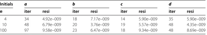
From Table , we see that the test results forλ∈(, ) are better than for other cases. Especially, the good numerical results are obtained whenλcloses to . Then we compare the test results with Chen and Pan [], where we setp= ,ε= .e–,σ= .e–,β= . for convenience. Table lists the test results for [].
Tables and indicate that Algorithm performed much better than Chen and Pan [] did on Problem .
Table 1 Test results for Problem 1
Initials a b c d
n λ iter resi iter resi iter resi iter resi
4 0.0001 3 1.61e–021 2 4.71e–012 3 1.42e–018 3 2.36e–016 0.001 3 4.84e–020 2 6.26e–012 3 1.37e–017 3 1.22e–015 0.03 3 3.81e–012 2 3.74e–010 3 2.11e–014 3 7.61e–013 0.05 3 3.15e–010 2 1.54e–009 3 1.76e–013 3 2.52e–012 0.1 4 1.21e–012 3 3.90e–012 3 1.20e–012 4 6.59e–010 0.5 4 8.78e–011 3 2.70e–010 3 8.18e–010 5 7.32e–013 1 4 3.31e–010 4 1.86e–017 4 1.66e–016 5 1.05e–012 1.3 4 5.23e–009 4 3.78e–013 4 1.92e–014 5 3.20e–011 1.5 5 1.36e–017 4 1.57e–012 4 2.07e–014 6 7.86e–016 2 5 2.22e–013 4 9.67e–011 4 3.05e–012 7 1.64e–016 3.2 6 1.77e–015 5 2.28e–011 4 1.36e–010 13 1.72e–011 3.5 6 4.69e–012 5 5.76e–009 4 5.97e–009 16 1.06e–010 3.8 7 1.62e–013 6 5.16e–011 4 6.87e–010 8 5.69e–013
10 0.0001 3 2.56e–017 2 4.37e–010 3 1.49e–018 3 5.27e–015 0.001 3 1.04e–016 2 4.84e–010 3 3.18e–017 3 5.15e–015 0.03 3 7.55e–011 2 5.42e–009 3 2.90e–014 3 7.16e–009 0.05 3 3.80e–009 3 3.01e–021 3 2.05e–013 3 5.87e–012 0.1 3 6.69e–009 3 1.03e–010 3 3.16e–012 4 7.08e–010 0.5 4 2.86e–010 3 3.91e–010 3 2.30e–009 5 3.87e–014 1 4 2.98e–009 4 1.47e–016 3 1.24e–009 5 7.37e–018 1.3 5 9.65e–018 4 1.25e–014 4 2.27e–013 5 1.49e–011 1.5 5 6.52e–017 4 2.08e–009 4 1.45e–013 6 8.19e–016 2 5 5.67e–014 5 3.91e–017 4 2.22e–014 6 7.76e–009 3.2 6 5.53e–014 5 5.85e–010 4 7.08e–009 13 2.23e–009 3.5 6 3.03e–011 6 7.13e–015 4 6.83e–010 20 1.12e–010 3.8 7 2.93e–013 6 2.81e–010 4 3.62e–010 8 8.00e–014
100 0.0001 3 9.91e–012 3 6.59e–022 3 2.43e–018 3 2.25e–011 0.001 3 1.41e–011 3 1.97e–021 3 3.31e–017 3 1.68e–011 0.03 4 7.16e–021 3 8.29e–018 3 3.25e–014 4 3.76e–019 0.05 4 6.93e–020 3 1.27e–016 3 1.13e–013 4 9.21e–017 0.1 4 8.22e–012 4 3.17e–021 3 3.05e–012 4 4.96e–010 0.5 5 8.60e–020 4 6.17e–019 3 3.00e–009 5 4.00e–011 1 5 2.57e–017 4 1.03e–014 3 2.55e–009 5 7.21e–018 1.3 5 1.11e–015 4 4.37e–011 4 1.00e–014 5 2.87e–009 1.5 5 1.63e–014 5 7.45e–016 4 1.42e–012 6 4.25e–017 2 5 8.25e–012 5 4.76e–014 4 4.63e–011 7 1.16e–013 3.2 6 7.28e–010 6 5.92e–011 4 2.88e–011 17 1.14e–014 3.5 7 2.78e–015 6 3.85e–009 4 3.11e–009 27 1.02e–009 3.8 7 7.03e–009 7 4.89e–013 4 3.62e–010 7 8.13e–012
Table 2 Test results for Chen and Pan [2] on Problem 1
Initials a b c d
n iter resi iter resi iter resi iter resi
4 34 4.92e–009 18 7.17e–009 14 5.90e–009 35 5.90e–009 10 48 6.79e–009 20 3.76e–009 19 5.57e–009 48 4.35e–009 100 97 9.58e–009 23 6.47e–009 18 9.34e–009 48 8.69e–009
Consider the following problem: findusuch that
⎧ ⎪ ⎪ ⎪ ⎪ ⎪ ⎨ ⎪ ⎪ ⎪ ⎪ ⎪ ⎩
u≥ in,
–u+f(u,x,y) – (y– .)≥ in, u(–u+f(u,x,y) – (y– .)) = in,
[image:10.595.118.480.560.622.2]wheref(u,x,y) is a continuously differentiableP-function. We discretize the problem by
the five-point difference scheme with mesh-steph. Then we get the following comple-mentarity problem: findx∈Rnsuch that
x≥, Ax+(x)≥ and xT Ax+(x)= .
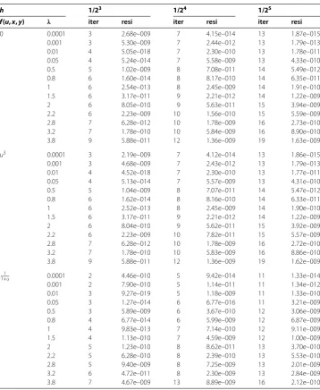
Set initial point asx= (, . . . , )T. Table lists the test results with different functionsf,
λ, andh.
From Table , we have the following observations.
[image:11.595.118.477.296.733.2]• Our test results become better whenλdecreases. It is obvious that whenλ= the result is not good enough. That is to say, Algorithm with the NCP-functionφλ
Table 3 Test results for Problem 2
h 1/23 1/24 1/25
f(u,x,y) λ iter resi iter resi iter resi
0 0.0001 3 2.68e–009 7 4.15e–014 13 1.87e–015
0.001 3 5.30e–009 7 2.44e–012 13 1.79e–013
0.01 4 5.05e–018 7 2.30e–010 13 1.78e–011
0.05 4 5.24e–014 7 5.58e–009 13 4.33e–010
0.5 5 1.02e–009 8 7.08e–011 14 5.49e–012
0.8 6 1.60e–014 8 8.17e–010 14 6.35e–011
1 6 2.54e–013 8 2.45e–009 14 1.91e–010
1.5 6 3.17e–011 9 2.21e–012 14 1.22e–009
2 6 8.05e–010 9 5.63e–011 15 3.94e–009
2.2 6 2.23e–009 10 1.56e–010 15 5.59e–009
2.8 7 6.28e–012 10 1.78e–009 16 2.73e–010
3.2 7 1.78e–010 10 5.84e–009 16 8.90e–010
3.8 9 5.88e–011 12 1.36e–009 19 1.63e–009
u3 0.0001 3 2.19e–009 7 4.12e–014 13 1.86e–015
0.001 3 4.68e–009 7 2.43e–012 13 1.79e–013
0.01 4 4.52e–018 7 2.30e–010 13 1.77e–011
0.05 4 5.13e–014 7 5.57e–009 13 4.31e–010
0.5 5 1.04e–009 8 7.07e–011 14 5.47e–012
0.8 6 1.62e–014 8 8.16e–010 14 6.33e–011
1 6 2.52e–013 8 2.45e–009 14 1.90e–010
1.5 6 3.17e–011 9 2.21e–012 14 1.22e–009
2 6 8.04e–010 9 5.62e–011 15 3.92e–009
2.2 6 2.23e–009 10 7.82e–011 15 5.57e–009
2.8 7 6.28e–012 10 1.78e–009 16 2.72e–010
3.2 7 1.78e–010 10 5.83e–009 16 8.86e–010
3.8 9 5.88e–011 12 1.36e–009 19 1.62e–009
1
1+u 0.0001 2 4.46e–010 5 9.42e–014 11 1.33e–014
0.001 2 7.90e–010 5 1.14e–011 11 1.34e–012
0.01 3 9.27e–019 5 1.18e–009 11 1.33e–010
0.05 3 1.27e–014 6 6.77e–016 11 3.21e–009
0.5 3 5.89e–009 6 3.67e–010 12 3.06e–009
0.8 4 6.77e–014 6 5.99e–009 12 6.87e–009
1 4 9.83e–013 7 7.14e–010 12 9.11e–009
1.5 4 1.13e–010 7 4.59e–009 12 1.00e–009
2 5 1.23e–010 8 8.62e–011 13 3.70e–010
2.2 5 6.28e–010 8 2.39e–010 13 5.53e–010
2.8 5 9.40e–009 8 7.25e–009 13 2.01e–009
3.2 6 4.72e–011 8 2.30e–009 13 2.84e–009
Table 4 Test results for Sun and Zeng [10] on Problem 2
h 1/23 1/24 1/25
f(u,x,y) iter resi iter resi iter resi
0 5 6.45e–016 8 3.11e–015 14 5.03e–011
u3 5 8.12e–009 9 1.20e–012 15 3.86e–008
1
[image:12.595.118.479.192.301.2]1+u 5 1.89e–009 8 7.92e–010 14 1.13e–007
Table 5 Test results for MCPLIB problems
λ 1.5 2 3
Problem iter time iter time iter time
mathinum(1) 4 0.048 4 0.050 5 0.050
mathinum(2) 4 0.031 5 0.028 6 0.036
mathinum(3) 7 0.030 7 0.030 8 0.032
mathinum(4) 6 0.076 7 0.074 7 0.080
nash(1) 7 2.536 8 2.538 11 2.529
nash(2) 8 2.284 9 2.301 13 2.334
tobin(1) 7 16.878 9 16.729 10 17.321
tobin(2) 12 17.389 14 17.342 16 17.358
( <λ< ) is better than the one discussed in [] where the Fischer-Burmeister function was used.
• Whether the functionf(u,x,y)is linear or nonlinear, the test results are good. The results are especially better whenλcloses to.
We compare the test results with Sun and Zeng [] where we setβ= .,c= .. Table
lists the test results for [] with different functionsf andh.
Tables and indicate that Algorithm performed as well as Sun and Zeng [] did on Problem .
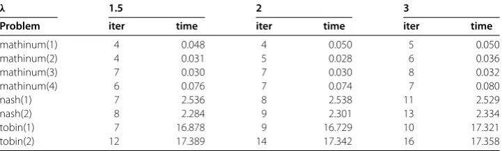
Problem We implemented Algorithm for some test problems with all available start-ing points in MCPLIB []. The results are reported in Table with seconds for unit of time.
The above examples indicate that the results are better whenλcloses to . A reason-able interpretation for this is that the values ofgi(x,z) andhi(x,z) become smaller when λincreases and hence causes some difficulty for Algorithm . This also implies that the performance of Algorithm will become worse whenpincreases. Whenλ→, the NCP obviously reduces tomin{x,F(x)}= . But it is a nonsmooth equation so we cannot use this method.
6 Concluding remarks
In this paper, we have studied a class of one-parametric NCP-functionsφλ(·,·) which in-clude the well-known Fischer-Burmeister function as a special case and proposed modi-fied Newton-type algorithms for solvingPcomplementarity problems.
Competing interests
The authors declare that they have no competing interests.
Authors’ contributions
WX participated in the design of the algorithm. ZD performed the numerical experiment and statistical analysis. All authors read and approved the final manuscript.
Acknowledgements
This work was supported by the NSFC (50975200).
Received: 24 February 2012 Accepted: 12 November 2012 Published: 7 December 2012
References
1. Chen, J-S: On some NCP-functions based on the generalized Fischer-Burmeister function. Asia-Pac. J. Oper. Res.24, 401-420 (2007)
2. Chen, J-S, Pan, S: A family of NCP functions and a descent method for the nonlinear complementarity problem. Comput. Optim. Appl.40, 389-404 (2008)
3. Fischer, A: A special Newton-type optimization methods. Optimization24, 269-284 (1992)
4. Hu, SL, Huang, ZH, Chen, J-S: Properties of a family of generalized NCP-functions and a derivative free algorithm for complementarity problems. J. Comput. Appl. Math.230(1), 69-82 (2009)
5. Hu, SL, Huang, ZH, Lu, N: Smoothness of a class of merit functions for the second-order cone complementarity problem. Pac. J. Optim.6(3), 551-571 (2010)
6. Kanzow, C, Kleinmichel, H: A new class of semismooth Newton-type methods for nonlinear complementarity problems. Comput. Optim. Appl.11, 227-251 (1998)
7. Lu, LY, Huang, ZH, Hu, SL: Properties of a family of merit functions and a derivative-free method for the NCP. Appl. Math. J. Chin. Univ. Ser. A25(4), 379-390 (2010)
8. Yamashita, N, Fukushima, M: Modified Newton methods for solving a semismooth reformulation of monotone complementarity problems. Math. Program.76, 469-491 (1997)
9. Qi, L: Convergence analysis of some algorithms for solving nonsmooth equations. Math. Oper. Res.18, 227-244 (1993) 10. Sun, Z, Zeng, JP: A monotone semismooth Newton type method for a class of complementarity problem. J. Comput.
Appl. Math.235, 1261-1274 (2011)
11. Billups, SC, Dirkse, SP, Soares, MC: A comparison of algorithms for large scale mixed complementarity problems. Comput. Optim. Appl.7, 3-25 (1997)
doi:10.1186/1029-242X-2012-286