Optimization of Shell and Tube Heat Exchangers for Sea Water Cooling by COMSOL Multiphysics

(1)

International Journal of Emerging Technology and Advanced Engineering

Website: www.ijetae.com (ISSN 2250-2459, Volume 2, Issue 11, November 2012)

264

Optimization of Shell and Tube Heat Exchangers for Sea Water

Cooling by COMSOL Multiphysics

S. Swaraj Reddy

1

, Tania Dey

2

, Haribabu K

3

, Harshit Krishnakumar

4

, Garima Vishal

5

1,2,4,5

Students, Department of Chemical Engineering, National Institute of Technology Calicut, Kozhikode.

3_{Assistant Professor, Department of Chemical Engineering, National Institute of Technology Calicut, Kozhikode.}

Abstract —In this paper, the new approach of COMSOL Multiphysics 3.5, a commercial finite element modelling software has been employed to simulate a theoretical (2-D geometry) model for shell and tube heat exchanger. The model incorporates the effects of fluid velocity in inlet and outlet and the material used for construction of heat exchanger for the required heat transfer to be achieved. The purpose of this paper is optimization of shell and tube heat exchanger for sea water cooling operation. In this operation, the coolant media from industries and other sources, at 120C has to be cooled to 60C using deep sea water available at 2 to 50C. The study mainly focuses on various configurations of shell and tube heat exchanger and the effect of different variables on heat transfer rate for optimized configuration. Simulation results show that aluminium is obtained as the preferred material of selection as it is coherent with all the parameters of design for the desired heat transfer.

Keywords — Comsol Multiphysics, Heat Transfer rate, Optimization, Sea Water Cooling, Shell and tube heat exchanger.

I. INTRODUCTION

There is an overwhelming demand for air conditioning in office buildings. Consequently, the amount of energy used for cooling is a concern for many. The increased demand for cooling also means that more are being installed on the rooftops of buildings.

If the building is situated near a sea, one option could be to use the seawater as a heat sink, eliminating the need for a conventional air conditioner. Furthermore, by using seawater for cooling the condenser, a saving of up to 90%of energy can be achieved [1].

Seawater cooling systems are often designed using an intermediate heat exchanger that separates the sea water and the cooling media in the system, in order to prevent contamination of the condenser [2].

This technology has been put into use in several places around the world. It has been proposed to cool buildings in downtown Toronto using cold, deep-water withdrawn from Lake Ontario in North America [3].

A unique Sea Water Cooling (SWC) system at the National Oceanography Centre (NOC), located in Southampton's dock area, UK, is saving energy and helping to reduce the building's carbon footprint [4]. Some preliminary research has been done on the use of sea water district heating and cooling for Tallinn coastal area, Finland [5]. Such a plant has also been installed in the Ninghai Power Plant, China [6].

With the increasing use of computers, powerful simulation software has become more popular. Computer simulation provides a lucid picture of the complicated physical phenomena that occur in any chemical engineering processes. This is possible because these simulations are able to provide visual representation of otherwise hard to picture concepts such as, concentration gradients, velocity profiles and temperature gradients [7]. Although there is no

substitute for laboratory run experiments, digital

simulations can be used as the stepping stone towards a better understanding of basic chemical engineering principles.

One such software is COMSOL Multiphysics. COMSOL Multiphysics is a finite element analysis, solver and Simulation software, Finite Element Software package for various physics and engineering applications, especially coupled phenomena, or Multiphysics. It is good at modeling chemical engineering phenomenon since it is designed to combine or couple several processes (like heat and momentum transfer in case of shell and tube heat exchanger) in a single model. Thus, COMSOL can solve multiple nonlinear PDE’s simultaneously and the models can be generated and solved in one, two or even three

dimensions. Furthermore, COMSOL models are

interactive, user friendly and they are ideal tools to complement theoretical knowledge.

Nomenclature

U velocity scale L length scale

(2)

International Journal of Emerging Technology and Advanced Engineering

265

Cp specific heat capacity (J/(kg·K))

T temperature (K)

k thermal conductivity (W/(m·K)) ρ density (kg/m3)

µ Velocity vector (m/s)

Q sinks or source term

kT turbulent thermal conductivity µT turbulent dynamic viscosity

PrT turbulent Prandtl number.

ῡ velocity field in two dimensional rectangular Cartesian coordinate system

E total energy

keff effective thermal conductivity

Sh source

(Tij)eff deviatory stress tensor.

II. COMSOL MULTIPHYSICS

COMSOL Multiphysics was originally known as FEMLAB because it uses the finite element method to analyse and solve complex problems.

The software comes with several modules in its library for specific applications. These applications include: AC/DC Module, Acoustics Module, CAD Import Module, Chemical Engineering Module, Earth Science Module, Heat Transfer Module, Material Library, MEMS Module, RF Module, and Structural Mechanics Module. Each module contains modelling tools and equations for the application described. Modelling tools from multiple modules can be coupled together to accurately depict complicated systems and processes [8].

A. Chemical Engineering Module

The Chemical Engineering Module is the perfect tool for process-related modeling. It is specifically designed to easily couple transport phenomena— computational fluid dynamics (CFD) or mass and energy transport—to chemical reaction kinetics. It can be used for the modeling of reactors, filtration and separation units, heat exchangers, and other equipment common in the chemical industry. Other modeling interfaces account for electrochemical systems (such as fuel cells) and applications where electric fields influence transport, such as electrophoresis and electro kinetic flow.

Models may be created in 1, 2, or 3 dimensions, and use partial differential equations to relate the physics of each aspect of a model. In order to simulate all the aspects of a system, multiple models are often necessary [8].

B. Using COMSOL

The first step to creating a model using COMSOL is to create the desired geometry to be evaluated. This can be 1, 2, or 3 dimensional geometries. Irregular geometries are also possible to be made using the various drawing tools available to COMSOL. The next step is to mesh the model. This involves breaking the geometry into subsections that will be evaluated individually and then displayed together to give an overview of the phenomena taking place. It is generally most effective to specify a small mesh size at and near boundaries as this is where the most irregularities will occur. After meshing, the physics of the model may be defined both throughout the sub domain of the model and at each of the boundaries. The model can then be solved and post-processing can occur. Post-processing involves manipulating the solution to obtain plots for relevant data and fluxes. Parametric studies can then be performed in order to optimize the model [8].

III. PROBLEM DESCRIPTION

The objective of this project is to create a COMSOL model for shell and tube heat exchanger. Sea water cooling plant operation is taken into consideration. In this, sea water at 2 to 50C is used to cool the cooling medium. The cooling medium is available at 120C, which is to be cooled to 60C. A decrease of 60C is desired from the heat transfer in heat exchanger. The project also aims at plotting and studying the temperature and velocity profile for different inlet flow velocity, pipe diameter and pipe material.

The shell and tube heat exchanger is considered here because this type of heat exchanger is cheap and easily available. There is flexibility regarding materials of construction. The shell and the tubes can be made of different materials. Cleaning and repair is relatively straightforward.

(3)

International Journal of Emerging Technology and Advanced Engineering

266

IV. METHODOLOGY

A. Governing Equations

1. Selection of governing physics:

An important characteristic of the flow is the Reynolds number, Re, defined as

If the Reynolds number is low, the flow is dominated by viscous forces, so Low Reynolds Number k-å model (LRN) can be used in COMSOL [9]. If, on the other hand, the Reynolds number is high, then the flow is dominated by inertial forces and turbulent flow occurs. Since we are referring to the sea water cooling operation we study the flow pattern in it and conclude it to be turbulent hence K-Ɛ

turbulence model is considered. Thus, the governing equations in this model are

a) The Reynolds-averaged Navier-Stokes (RANS)

equations and a k-Ɛ turbulence model b) General Heat transfer equations

The Non-Isothermal Flow interface was selected; thus the above equations are coupled to model the fluid-thermal interaction.

The governing equation for heat transfer in the model is the heat equation for conductive and convective heat transfer

( )

The temperature-dependent properties for water and metals from the built-in material library were used in the model. The software incorporates the influence of the turbulent fluctuations on the temperature field by using the Kays-Crawford model for the turbulent Prandtl number.

So the equation for heat transfer in solids is given by

( )

Furthermore, to account for the effect of mixing due to eddies, it is necessary to correct the fluid’s thermal conductivity. The turbulence results in an effective thermal conductivity, keff, according to the equation.

2. Continuity equation:

Since mass is conserved within the control volume or infinitesimal fluid element, the rate of increase of mass within a volume is equal to the net rate at which mass crosses its bounding surface.

The conservation of mass can be defined by a scalar equation. Velocity components in x, y and z directions are represented by u, v, and w. The components of velocity vector are functions of space and time. The continuity equation is given by

( )

The second term is divergence of the velocity and named as convective term. It represents the difference between the mass flows into and the mass flows out from boundaries. It must be balanced with the first term which describes the accumulation. If the fluid is incompressible, then density is constant in both location and time.

3. Energy equation in the k- Ɛ models:

( )

{

(

)

}

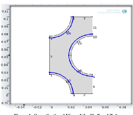
Term contains contributions from radiation, as well as any other volumetric heat sources [10].

B. Geometry of Shell and Tube HeatExchanger

[image:3.612.330.556.438.634.2]

Considering a single section of it in 2-D gives the following figure

Figure 1: Cross Sectional View of the Shell and Tube

C. Boundary Conditions

The boundary conditions mentioned for the problem are A. K-Ɛturbulence equations in the fluid domain:

a. Specified initial velocity

(4)

International Journal of Emerging Technology and Advanced Engineering

267

c. Wall function at the pipe/water interfaces d. Fixed outlet pressure

B. Heat transport equations:

a. Fixed temperature at the inlet

b. Convection-dominated transport at the outlet c. Symmetry (thermal insulation) at the region

borders

d. Thermal wall function at the pipe/water interfaces

e. Fixed temperature at the inner pipe surfaces

Further, specific boundary conditions are given in table II.

D. Sub Domain Settings

The types of materials were loaded from the inbuilt material library present in COMSOL Multiphysics 3.5.

Both the liquids used were water, and the pipe materials were steel AISI 4030 and simple aluminium. The sub domains of pipe were identified and selected, and the pipe material was fixed. The fluids sub domain were identified and given the properties of water. Further, for each case, the material of pipe is changed. The specific sub domain for each case is given in tables II. The water is common in all cases.

E. Meshing

There are different types of meshing. Selecting a mesh is purely intuitive.

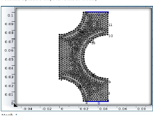
[image:4.612.323.566.128.319.2]

Default meshing was used for this model, because the temperature of the tube side fluid is fixed. This reduces the complexity of the problem. A default mesh with single refinement will give satisfactory results. The finished mesh will look like figure 2.

Figure 2: Meshed view of the shell and tube

TABLEI

MESH STATISTICS FOR SHELL AND TUBE

SNo. Property Value

1 Minimum element quality 0.7512

2 Average element quality 0.9511

3 Triangular elements 1956

4 Edge elements 202

F. Solving the problem

[image:4.612.40.574.567.706.2]

There are a wide range of solvers to select from in COMSOL. For all of our simulations, the auto select of solver was used, which detects the type of problem encountered and automatically selects the best solver apt for the given problem. The solver detected was stationery segregated solver, and the same solver was used in all our simulations.

TABLE II

Parameters for Shell and Tube

SNo. Flow rate

(hot fluid)(m3/s)

Mass flow

rate(kg/s)

Pipe temp

Cold fluid(sea water) (K)

Pipe material Inlet temp Hot fluid(K)

Hot fluid Outlet temp obtained(K)

Case1 0.01 0.247 278 Steel AISI 4340 285 282.6

Case 2 0.001 0.0247 278 Aluminium 285 279.2

Case3 0.001 0.0247 278 Steel AISI 4340 285 279.4

(5)

International Journal of Emerging Technology and Advanced Engineering

268

There are different types of meshing. Selecting a mesh is purely intuitive.

V. RESULT AND DISCUSSION

A. Shell and Tube Heat Exchanger

[image:5.612.334.569.137.334.2]

A cross section of the Shell and tube heat exchanger was taken and used for the purpose of simulation in the COMSOL software. The parameters studied were Flow rate of the hot fluid, material of pipe and the tube diameter. Keeping the inlet temperatures and flow rates constant, the flow rate was adjusted by hit and trial to get the desired outlet temperature. The optimum flow rate for each case had been found, and recorded. The following four cases were considered. The same data has been taken from the sea water cooling operation. The diameter of the inflow boundary was set as 0.025 m.

Figure 3: Boundary consideration of shell and tube for temperature measurement

In each of the cases, the temperature plot is given for the red line highlighted boundary.

1. Case 1:

In this, the hot fluid is taken in the annulus and cold in inner pipe (constant temperature 278 K). For the given flow rate of hot fluid 0.01 m/s, with pipe material Steel AISI 4340 the temperature difference achieved is 2.4 K. The temperature profiles are (the red line is the basis for the graph plotted)

Figure 4: Temperature vs. Arc length curve

Figure 5: Surface plot of Temperature

2. Case 2:

[image:5.612.56.277.340.480.2]

(6)

International Journal of Emerging Technology and Advanced Engineering

[image:6.612.334.564.135.331.2]

269

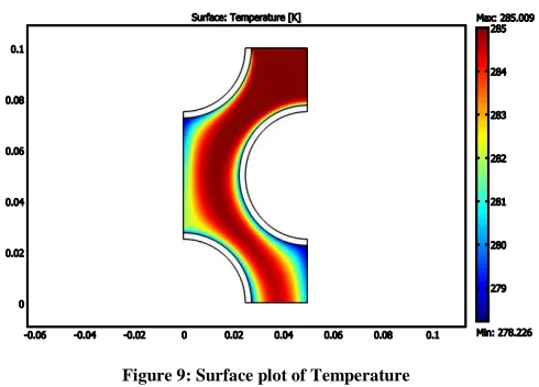
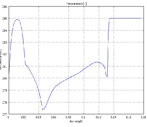
3. Case 3:

[image:6.612.58.293.137.331.2]

In this, the hot fluid is taken in the annulus and cold in inner pipe (constant temperature 278 K). For the given flow rate of hot fluid 0.001 m/s, with pipe material Steel AISI 4340 the temperature difference achieved is 5.6 K. The temperature profiles are (the red line is the basis for the graph plotted)

4. Case 4:

[image:6.612.49.295.356.543.2] [image:6.612.323.568.357.533.2]

(7)

International Journal of Emerging Technology and Advanced Engineering

[image:7.612.60.296.136.340.2]

270

VI. CONCLUSION

In the simulation of the shell and tube heat exchanger, the materials and flow rates were changed accordingly. In case 1 and 3 the material is kept constant and flow rate is optimized. Then in the case 2 taking the better flow rate, material is changed and in case 3 taking the optimum flow rate and the better material the desired temperature drop is found out. Considering the plant economy and requiring the above cases are considered helpful.

The project is based on doing multiple simulations by assuming parameter values for each case. Such studies can now be performed in the modified versions of COMSOL 4.2a, as parametric studies.

This feature is very helpful in determining the optimum dimensions. There is no need to assume values and do hit and trial in the new version because of the introduction of parametric sweep. It solves using iterations of many random values thereby giving more accurate results.

Acknowledgment

This research was supported by Mr. Prithivi Raj J, Research Scholar in Department of chemical engineering, IIT Bombay. We take this opportunity to thank him. Special thanks to him for rendering his full support to carry out the simulations.

REFERENCES

[1] Bluerise, “Seawater Air Conditioning”, 2012, (http://www.bluerise.nl/technology/seawater-air-conditioning-swac. [2] Dan V. Bomholt Andersen, “Seawater cooling", Hot|Cool, 1/2004

(2004).

[3] Farrell M. Boyce, Paul F. Hamblin, L.D. Danny Harvey, William M. Schertzer, R. Craig McCrimmon, “Response of the ThermalStructure of LakeOntario to DeepCoolingWaterWithdrawals and to GlobalWarming”, Journal of Great Lakes Research, Vol. 19, Issue 3, pp. 603-616 (1993).

[4] Natural Environmental Research Council, “Seawater cools National Oceanography Centre”, June 17th_, _2011, (http://www.nerc.ac.uk/about/work/policy/green/achievements/seaw ater.asp).

[5] Hani and T. Koiv, "The Preliminary Research of Sea Water District Heating and Cooling for Tallinn Coastal Area," Smart Grid and Renewable Energy, Vol. 3 No. 3, 2012, pp. 246-252. doi: 10.4236/sgre.2012.33034.

[6] Zhou Daji,Zhang Hualun,Ji Jun, “Optimization and Innovation of Engineering Design for Ninghai Power Plant”, February 2011, doi: CNKI:SUN:DIPI.0.2011-02-011.

[7] ShubhneetKaurSandhu, “COMSOL Assisted Modeling of a Climbing Film Evaporator”, (August 27, 2010).

[8] Nicholas Bartal, Gabriella Serrati,Daniel Szewczyk, John Waterman, “Modeling of a Catalytic Packed Bed Reactor and Gas Chromatograph Using COMSOL Multiphysics”, (April 24, 2009). [9] J. D. Freels, I. T. Bodey, R. V. Arimilli, F. G. Curtis, K. Ekici, P. K.

Jain, “Preliminary Multiphysics Analyses of HFIR LEU Fuel Conversion using COMSOL”, (June, 2011).