www.hydrol-earth-syst-sci.net/20/529/2016/ doi:10.5194/hess-20-529-2016
© Author(s) 2016. CC Attribution 3.0 License.
Integrated water system simulation by considering hydrological and
biogeochemical processes: model development, with parameter
sensitivity and autocalibration
Y. Y. Zhang1, Q. X. Shao2, A. Z. Ye3, H. T. Xing4, and J. Xia1
1Key Laboratory of Water Cycle and Related Land Surface Processes, Institute of Geographic Sciences and Natural Resources Research, Chinese Academy of Sciences, Beijing, 100101, China
2CSIRO Digital Productivity Flagship, Leeuwin Centre, 65 Brockway Road, Floreat Park, WA 6014, Australia 3College of Global Change and Earth System Science, Beijing Normal University, Beijing, 100875, China 4CSIRO Agriculture Flagship, GPO BOX 1666, Canberra, ACT 2601, Australia
Correspondence to: Y. Y. Zhang ([email protected]) and Q. X. Shao ([email protected])
Received: 1 April 2015 – Published in Hydrol. Earth Syst. Sci. Discuss.: 22 May 2015 Revised: 11 December 2015 – Accepted: 21 December 2015 – Published: 1 February 2016
Abstract. Integrated water system modeling is a feasible ap-proach to understanding severe water crises in the world and promoting the implementation of integrated river basin man-agement. In this study, a classic hydrological model (the time variant gain model: TVGM) was extended to an integrated water system model by coupling multiple water-related pro-cesses in hydrology, biogeochemistry, water quality, and ecology, and considering the interference of human activ-ities. A parameter analysis tool, which included sensitivity analysis, autocalibration and model performance evaluation, was developed to improve modeling efficiency. To demon-strate the model performances, the Shaying River catchment, which is the largest highly regulated and heavily polluted tributary of the Huai River basin in China, was selected as the case study area. The model performances were evaluated on the key water-related components including runoff, wa-ter quality, diffuse pollution load (or nonpoint sources) and crop yield. Results showed that our proposed model simu-lated most components reasonably well. The simusimu-lated daily runoff at most regulated and less-regulated stations matched well with the observations. The average correlation coeffi-cient and Nash–Sutcliffe efficiency were 0.85 and 0.70, re-spectively. Both the simulated low and high flows at most stations were improved when the dam regulation was consid-ered. The daily ammonium–nitrogen (NH4–N) concentration was also well captured with the average correlation coeffi-cient of 0.67. Furthermore, the diffuse source load of NH4–N
and the corn yield were reasonably simulated at the admin-istrative region scale. This integrated water system model is expected to improve the simulation performances with ex-tension to more model functionalities, and to provide a sci-entific basis for the implementation in integrated river basin managements.
1 Introduction
de-530 Y. Y. Zhang et al.: Integrated water system simulation velopment of water-related sciences, computer science, Earth
observation technologies and the availability of open data. The hydrological cycle has been known as a critical link-age among other water-related processes (e.g., physical, bio-geochemical and ecological processes) and energy fluxes at the basin scale (Burt and Pinay, 2005). For example, physi-ological and ecphysi-ological processes of vegetation affect evap-otranspiration, soil moisture distribution and nutrient move-ment. In the meantime, soil moisture and nutrient constrain the vegetation growth. Overland flow is a carrier of pollu-tants to water bodies. Therefore, all the processes should be considered simultaneously to capture the interactions and feedbacks between individual cycles. Multidisciplinary re-search provides an effective way to enable breakthroughs in the integrated water system modeling by integrating the theo-ries in water-related sciences (e.g., accumulated temperature law for phenological development, Darcy’s law for ground-water flow, Saint-Venant equation for flow routing, balance equation for mass and momentum, Richards’ equation for unsaturated zone, Horton theory for infiltration, Penman– Monteith equation for evapotranspiration). Abundant open data sources further support the implementation of an inte-grated water system model, e.g., high-resolution spatial in-formation data, chemical and isotopic data from field exper-iments (Singh and Woolhiser, 2002; Kirchner, 2006).
Several models have been developed since the 1980s (Di Toro et al., 1983; Brown and Barnwell, 1987; Johnsson et al., 1987; Hamrick, 1992; Li et al., 1992; Abrahamsen and Hansen, 2000; Tattari et al., 2001; Singh and Wool-hiser, 2002). Owing to the complexity of the integrated wa-ter system and the scale conflicts between different pro-cesses, most existing models focus on only one or two major water-related processes, and can be categorized into three major classes. (1) Hydrological models emphasize the rainfall–runoff relationship and link with some dominating water quality and biogeochemical processes. These mod-els generally show satisfactory performances in simulating the hydrological processes. Some widely accepted models are TOPMODEL (Beven and Kirkby, 1979), SHE (Abbott et al., 1986), HSPF (Bicknell et al., 1993), VIC (Liang et al., 1994), ANSWERS (Bouraoui and Dillaha, 1996), HBV-N (Arheimer and Brandt, 1998, 2000), HYPE (Lindström et al., 2010) and its improved version S-HYPE (Strömqvist et al., 2012). (2) Water quality models focus on the migra-tion and transformamigra-tion processes of pollutants in water bod-ies. These models can simulate the water quality variables at high spatial and temporal resolutions in river networks by adopting multi-dimensional dynamic equations. However, they have difficulties in simulating the overland processes of water and pollutants. Typical models include WASP (Di Toro et al., 1983), QUAL2E (Brown and Barnwell, 1987) and EFDC (Hamrick, 1992). (3) Biogeochemical models have advantages in simulating the physiological and ecological processes of vegetation and the vertical movements of nu-trients and water in soil layers at the field or experimental
catchment scales. However, these models lack accurate hy-drological features (Deng et al., 2011) and are hard to simu-late the movements of water, nutrients and their losses along flow pathways in the basin. Some biogeochemical models are SOILN (Johnsson et al., 1987), EPIC (Sharpley and Williams, 1990), DNDC (Li et al., 1992), Daisy (Abraham-sen and Han(Abraham-sen, 2000) and ICECREAM (Tattari et al., 2001). Overall, most models usually achieve good performances on their oriented processes and only approximate the results for other processes outside of the model’s focus in the integrated river basin management. An important scientific question is “does including these extra processes in an integrated manner improve model results compared to models that are focused only on one component?”
SWAT is an integrated water system model that can simu-late most water-resimu-lated processes over a long period at large scales (Arnold et al., 1998). However, not all water-related processes can be well captured in practice because of the in-accurate descriptions of some processes, such as daily ex-treme flow events (Borah and Bera, 2004), soil nitrogen and carbon (Gassman et al., 2007) and regulation rules of dams or sluices in regulated basins (Zhang et al., 2013). Particularly, the simulation methods of surface runoff yield in SWAT have been questioned, e.g., the general applicability of the curve number (Rallison and Miller, 1981) and the scale limitations of the Green-Ampt infiltration model (King et al., 1999). Furthermore, SWAT has difficulties in accurately capturing the complicated dynamic processes of soil nitrogen and car-bon by comparing with other biochemical models (Gassman et al., 2007). Several modified versions have been devel-oped, such as SWIM (Krysanova et al., 1998) and SWAT-N (Pohlert et al., 2006).
In this study, we tended to develop an integrated water sys-tem model based on a hydrological model. The time variant gain model (TVGM) proposed by Xia (1991) is a lumped hydrological model based on the rainfall and runoff obser-vations from many basins with different scales all over the world. In the TVGM, the rainfall–runoff relationship is con-sidered to be nonlinear because the surface runoff coefficient varies over time and is significantly affected by antecedent soil moisture. The TVGM has a strong mathematical basis because this nonlinear relationship is transformed into a com-plex Volterra nonlinear formulation. Wang et al. (2002) ex-tended the TVGM to the distributed time variant gain model (DTVGM) by taking advantage of better computing facilities and available data sources. Currently, the DTVGM performs well in many basins with different scales and climate zones to investigate the effect of human activities and climate change on runoff (Xia et al., 2005; Wang et al., 2009).
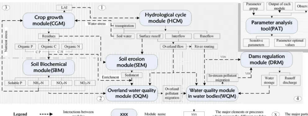
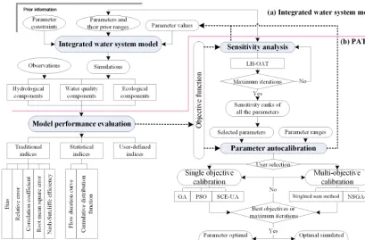
Figure 1. The model structure and the interactions among the major modules (1: hydrological part; 2: water quality part; 3: ecological part; 4: dam regulation part; 5: PAT).
model was built by extending the DTVGM through coupling of the detailed interactions and linkages among hydrologi-cal, water quality, soil biogeochemical and ecological pro-cesses, as well as considering the prevalent regulations of water projects (dams and sluices) at the basin scale. In or-der for reaor-ders to use the proposed model easily, a parameter analysis module, which included popular objective functions, autocalibration approaches and summary statistics, was also developed. To demonstrate the model performances, we sim-ulated several key water-related components including flow regimes, diffuse source (or nonpoint source) pools of nutri-ents, water quality variables in water bodies and crop yield in a highly regulated and heavily polluted catchment (Shaying River catchment) in China.
2 Methods and material 2.1 Model framework
Our proposed model includes eight major modules, namely the hydrological cycle module (HCM), soil biochemical module (SBM), crop growth module (CGM), soil erosion module (SEM), overland water quality module (OQM), wa-ter quality module of wawa-ter bodies (WQM) and dam reg-ulation module (DRM). The parameter analysis tool (PAT) is also designed for model calibration. The model struc-ture is shown in Fig. 1. More detailed descriptions of each module and its interactions with other modules are given in Sects. 2.1.1 to 2.1.5. The main equations of each module are deferred to the Appendix and Supplement for readers who are interested in the mathematical details.
Our model is based on the hypothesis that the cycles of wa-ter and nutrients (N, P and C) are inseparable and act as the critical linkages among all the modules. It takes full
advan-tage of the existing models, i.e., the powerful interconnec-tions of the hydrological models with other processes at the spatial scale, the elaborative descriptions of the ecological models on nutrient vertical movement in soil layers, and the elaborative descriptions of the water quality models on nutri-ent movemnutri-ents along river networks. First, several key com-ponents, simulated by the hydrological cycle module (HCM) (e.g., evapotranspiration, soil moisture and flow), are treated as critical linkages in all the modules (Sect. 2.1.1). Second, the soil biochemical processes determine the nutrient loads absorbed in the crop growth process (CGM) and migrated into water bodies as the diffuse pollution source (OQM and WQM). The accurate descriptions of soil biochemical pro-cesses are helpful in improving the simulation of diffuse source processes in responding to agricultural management (Sect. 2.1.2). Third, the hydrological cycle module (HCM) provides a function for describing the connections between spatial calculation units to simulate the overland and in-stream movements of water and nutrients at the basin scale (Sects. 2.1.1 and 2.1.3).
2.1.1 Hydrological cycle module (HCM)
532 Y. Y. Zhang et al.: Integrated water system simulation
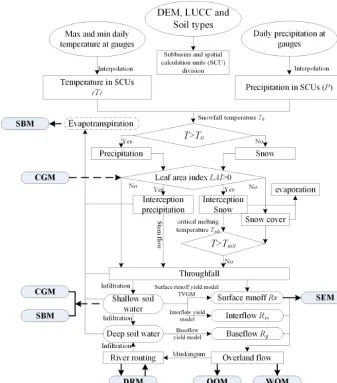
Figure 2. The flowchart of HCM and the interactions with other modules.
surface soil residues (Neitsch et al., 2011). The yields of in-terflow and baseflow have linear relationships with the soil moisture in the upper and lower layers, respectively (Wang et al., 2009). The infiltration from the upper to lower soil layers is calculated using the storage routing method (Neitsch et al., 2011). The Muskingum method or kinetic wave equation is used for river flow routing.
Figure 2 shows that the shallow soil moisture from the hy-drological cycle module is a major factor that connects the crop growth module (to control crop growth) and the soil bio-chemical module (to control the vertical migration and reac-tion of nutrients in the soil layers). Plant transpirareac-tion is also linked to the soil biochemical module (to drive the vertical migration of nutrients in the soil layers). The surface runoff is linked to the soil erosion module, while the overland flow (surface runoff, interflow and baseflow) is connected to the overland water quality module (to drive the movements of nutrients and sediment along flow pathways) and the water quality module of water bodies (rivers and lakes) for runoff
routing. Moreover, the hydrological cycle module provides the inflows for individual dams or sluices in the dam regula-tion module.
2.1.2 Modules for ecological processes
The ecological processes are described in the soil biochemi-cal module and the crop growth module. The crop growth and soil biochemical processes directly affect the soil moisture, evapotranspiration, nutrient transformation and loss from the soil layers. Therefore, our model incorporates the water cy-cle, nutrient cycy-cle, crop growth and their key linkages. Soil biochemical module (SBM)
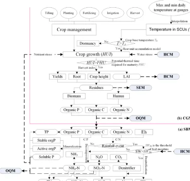
bio-Figure 3. The flowchart of SBM (a) and CGM (b) in the ecological part and the interactions with other modules.
chemical module are connected to the crop growth module as the nutrient constraints of crop growth and to the overland water quality module as the main diffuse sources to water bodies (Fig. 3a).
Soil C and N cycle. The sub-models of daily step
decom-position and denitrification in DNDC (Li et al., 1992) are adopted to simulate the soil biogeochemical processes of C and N at the field scale. The decomposition and other ox-idation processes are the dominant microbial processes in the aerobic condition. The three conceptual organic C pools are the decomposable residue C pool, microbial biomass C pool and stable C pool. The decomposition of each C pool is treated as the first-order decay process with the individual decomposition rates constrained by the soil temperature and moisture, clay content and C : N ratio. The major simulated processes of decomposition under aerobic conditions are mineralization, immobilization, ammonia (NH3) volatiliza-tion and nitrificavolatiliza-tion. The mineralizavolatiliza-tion and immobilizavolatiliza-tion of mineral N (NH+4 and NO−3) are determined by the flow rates of soil organic carbon (SOC) pools. NH3volatilization
is controlled by the NH+4 concentration, clay content, pH, soil moisture and temperature. NH+4 is oxidized to NO−3 dur-ing nitrification and nitrous oxide (N2O) is emitted into the air during the nitrification. Denitrification occurs under the anaerobic condition, which is controlled by soil moisture, temperature, pH and dissolved SOC content. The detailed de-scriptions are given in Appendix B and Li et al. (1992).
Soil P cycle. The major processes of the soil P cycle are
simulated according to the study of Horst et al. (2001). Six P pools are considered including three organic pools (sta-ble and active pools for plant uptake, a fresh pool associated with plant residue) and three mineral pools (dissolved min-eral, stable and active pools). The involved processes are the P release, mineralization and decomposition from fertilizer, manure, residue, microbial biomass, humic substances and the sorption by plant uptake (Horst et al., 2001; Neitsch et al., 2011).
[image:5.612.104.496.70.443.2]534 Y. Y. Zhang et al.: Integrated water system simulation
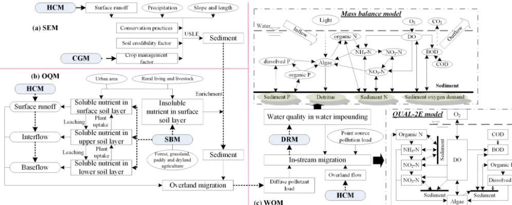
Figure 4. The flowchart of SEM (a), OQM (b) and WQM (c) in the water quality part and the interactions with other modules.
of which are consistent with the soil layers of the hydrolog-ical cycle module to smoothly exchange the values through the linkages (e.g., soil moisture) among different modules.
Crop growth module (CGM)
The crop growth module is developed based on the EPIC crop growth model (Hamrick, 1992). It simulates total dry matter, leaf area index, root depth and density distribution, harvest index, nutrient uptake, and so on (Williams et al., 1989; Sharpley and Williams, 1990). The crop respiration and photosynthesis drive the vertical movements of water and nutrients. The output of the leaf area index is a main factor connecting the hydrological cycle module (to control the transpiration), and the crop residue left in the fields is a main source of organic nutrients (C, N and P) connecting to the soil biochemical module for soil biochemical processes, to the overland water quality module and to the soil erosion module as one of the five constraint factors (Fig. 3b).
2.1.3 Modules for water quality processes
The water quality processes focus on the migration and trans-formation of water quality variables (e.g., sediment, different forms of nutrients, biochemical oxygen demand, BOD, and chemical oxygen demand, COD) along the flow pathways in the land surface and river network. The main modules are the soil erosion module for the sediment yield, the overland water quality module for the migration of overland diffuse source to water bodies and the water quality module for the migration and transformation of point and diffuse pollution sources in water bodies.
Soil erosion module (SEM)
The soil erosion by precipitation is estimated using the im-proved USLE equation (Onstad and Foster, 1975) based on runoff yields outputted from the hydrological cycle module and crop management factor outputted from the crop growth module. The soil erosion module simulates the sediment load for the overland water quality module to provide the carrier for the migration of insoluble organic matter along overland transport paths and water bodies (Fig. 4a).
Overland water quality module (OQM)
This module simulates the overland losses and migration loads of diffuse source pollutants (e.g., sediment, insoluble and dissolved nutrients, BOD and COD) (Fig. 4b). The main diffuse sources include the nutrient loss from the soil lay-ers and urban areas, and the farm manure from livestock in rural areas. The nutrient loss from the soil layers, as the pri-mary diffuse source in most catchments, is determined by the overland flow and sediment yield (Williams et al., 1989), and the other sources are estimated using the export coefficient method (Johnes, 1996). The overland migration processes contain the dissolved pollutant migration with overland flow and the insoluble pollutant migration with sediment. All the processes occur along the overland transport paths.
Water quality module of water bodies (WQM)
consid-ered. Point sources are directly added to the surface water in the model according to their geographic positions. Common point sources are urban water treatment plants and industrial plants.
Two modules are designed for the different types of water bodies, i.e., the in-stream water quality module and the water quality module for water impounding (reservoir or lake). The enhanced stream water quality model (QUAL-2E) (Brown and Barnwell, 1987) is adopted to simulate the longitudinal movement and transformation of water quality variables in the in-streams. The model is solved at the sub-basin scale rather than at the fine grid scale in order to maintain spatial consistency with the hydrological cycle module. The water quality outputs provide the water quality boundary of dams or sluices in the dam regulation module. The water quality module for water impounding assumes that water body is at the steady state and focuses on the vertical interaction of wa-ter quality processes. The main processes include wawa-ter qual-ity degradation and settlement, sediment resuspension and decay.
2.1.4 Dam regulation module (DRM)
Dams and sluices highly alter flow regimes and associated water quality processes in most river networks. Thus, the dam and sluice regulation should be considered in the wa-ter system models. The dam regulation module provides the regulated boundaries (e.g., water storage and outflow) to the hydrological cycle module for flow routing and to the water quality module of water bodies for pollutant migration.
Given that different types of dams and sluices are likely to show completely different regulation behaviors, we try to reproduce their common functionalities for either the flood control or water supply in this module. Three methods are proposed to calculate the water storage and outflow of dams or sluices, namely, the measured outflow, controlled outflow with target water storage and the relationship between out-flow and water storage volume. The first method requires users to provide the measured outflow series during the sim-ulation period. The second method simplifies the regsim-ulation rules of dams or sluices for long-term analysis based on the assumption that water is stored according to the usable wa-ter level during the non-flooding season and the flood control level during the flooding season, and the surplus water is dis-charged. This method requires the characteristic parameters of dam or sluice including water storage capacities of dead, usable, flood control and maximum flood levels and the cor-responding water surface areas. The third method is based on the relationships among water level, water surface area, storage volume and outflow according to the designed dam data or long-term observed data (Zhang et al., 2013) (Ap-pendix C).
2.1.5 Parameter analysis tool (PAT)
In our model, 66 lumped and 94 distributed parameters in-volve the hydrological, ecological and water quality pro-cesses. The distributed parameters are divided into 37 over-land parameters, 17 stream parameters and 40 parameters of water projects (only for the sub-basin with reservoir or sluice) according to their spatial distribution. These parame-ter values are deparame-termined by the properties of overland land-scape and soil, stream patterns and water projects, respec-tively. Different spatial calculation units share many common parameter values if their properties are the same.
Owing to a large number of parameters, it is hard to find optimal parameter values by manual tuning. The lim-ited number of observed processes causes equifinality in the model calibration (Beven, 2006). Therefore, the parameter sensitivity analysis and calibration are important steps to al-leviate equifinality in the applications of highly parameter-ized models, particularly for integrated water system models (Mantovan and Todini, 2006; Mantovan et al., 2007; McDon-nell et al., 2007). The PAT is designed for parameter sensi-tivity analysis, autocalibration and model performance eval-uation (Fig. 5).
To evaluate model performance, five traditionally used cri-teria are included in the PAT, i.e., bias (bias), relative error (re), root mean square error (RMSE), correlation coefficient (r) and Nash–Sutcliffe efficiency (NS defined by Nash and Sutcliffe, 1970). The detailed definitions of these criteria are given in Appendix D. Furthermore, flow duration curve and cumulative distribution function are also provided for captur-ing multiple signatures of calibrated processes. More criteria can also be proposed by the users. The objective function(s) to calibrate the model can be formed by single or multiple criteria or their function (such as weighted average).
The parameter analysis algorithms in the PAT include the parameter sensitivity method (Latin hypercube one factor at a time: LH-OAT) (van Griensven et al., 2006), the single objec-tive auto-optimization methods such as particle swarm opti-mization (PSO) (Kennedy, 2010), the genetic algorithm (GA) (Goldberg, 1989) and shuffled complex evolution (SCE-UA) (Duan et al., 1994), as well as the multi-objective auto-optimization methods such as the weighted sum method and nondominated sorting genetic algorithm II (NSGA-II) (Deb et al., 2002). The method can be selected on the basis of the specific requirements of users.
536 Y. Y. Zhang et al.: Integrated water system simulation
Figure 5. The flowchart of PAT and its interactions with other modules.
runoff coefficient (g1)for different land uses/covers is set in ascending order (water body, paddy land, urban area, forest, dryland agriculture, unused land and grassland). The inter-flow yield coefficient (Kss) is greater than the baseflow coef-ficient (Kbs). In the water quality module of water bodies, the settling rates of water quality variables (Kset)in the water im-pounding are greater than the resuspension rates (Kscu)and the settling rates (Rset)in channels. Second, the sensitive pa-rameters are determined to reduce the parameter dimensions by sensitivity analysis. Third, the selected sensitive param-eters are calibrated by the auto-optimization method, while the insensitive parameters remain as their default values that are given by referring to the literatures or other models (e.g., SWAT, EPIC and DNDC) in the same/similar basins.
The PAT connects with other modules through the param-eter values that are used to simulate the processes of other modules and evaluate the objective functions in sensitivity analysis and autocalibration. Depending on the algorithm used, the parameter values are (randomly) sampled from the multi-dimensional parameter spaces to drive our model, and the objective function value of each parameter set is then ob-tained. For the parameter sensitivity analysis, the sensitiv-ity index of each parameter set is evaluated by comparing the variation of the objective function value along with the change in parameter value. For the parameter autocalibra-tion, the good parameter sets are kept or updated by the auto-optimization method until the convergence or the maximum number of iterations is achieved.
2.2 Model operation 2.2.1 Multi-scale solution
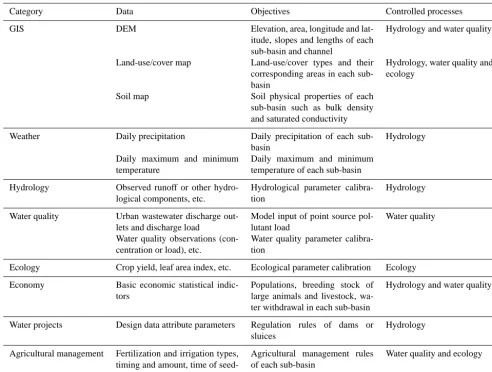
Table 1. The data sets and their categories used in the model.
Category Data Objectives Controlled processes
GIS DEM Elevation, area, longitude and
lat-itude, slopes and lengths of each sub-basin and channel
Hydrology and water quality
Land-use/cover map Land-use/cover types and their corresponding areas in each sub-basin
Hydrology, water quality and ecology
Soil map Soil physical properties of each sub-basin such as bulk density and saturated conductivity
Weather Daily precipitation Daily precipitation of each sub-basin
Hydrology
Daily maximum and minimum temperature
Daily maximum and minimum temperature of each sub-basin
Hydrology Observed runoff or other hydro-logical components, etc.
Hydrological parameter calibra-tion
Hydrology
Water quality Urban wastewater discharge out-lets and discharge load
Model input of point source pol-lutant load
Water quality
Water quality observations (con-centration or load), etc.
Water quality parameter calibra-tion
Ecology Crop yield, leaf area index, etc. Ecological parameter calibration Ecology
Economy Basic economic statistical indic-tors
Populations, breeding stock of large animals and livestock, wa-ter withdrawal in each sub-basin
Hydrology and water quality
Water projects Design data attribute parameters Regulation rules of dams or sluices
Hydrology
Agricultural management Fertilization and irrigation types, timing and amount, time of seed-ing and harvest, and crop types
Agricultural management rules of each sub-basin
Water quality and ecology
our model, these four land-use/cover units are divided into 10 specific categories of crop units as fallow for all these land-use/cover units, grass for grassland unit, fruit tree and non-economic tree for forest unit, early rice and late rice for paddy unit, spring wheat, winter wheat, corn and mixed dry crop for dryland agriculture unit. The crop unit of a specific land-use/cover pattern varies depending on crop cultivation structure and timing. The related modules are the soil bio-chemical module and the crop growth module. All of the outputs of the crop unit are summarized at the land-use/cover scale or sub-basin scale based on the area percentages in dif-ferent crop units.
For the temporal scale, it is practical to use a daily time step, as this is consistent with the underlying rainfall–runoff module and the data availability. The sub-daily scale may improve the performance in some modules (e.g., SEM and WQM). However, most observations (e.g., climate data sets, soil nutrient availability and water quality concentrations) are at the daily scale, leading to potential uncertainties or in-stabilities to disaggregate the observations into a sub-daily
scale. Linear or nonlinear aggregation functions are used to transform different timescales to daily scale (Vinogradov et al., 2011), such as exponential functions for flow infiltration and overland flow routing processes in the hydrological cycle module, for soil erosion processes in the soil erosion module (Eqs. A5, A6 and S32 in Appendix A and the Supplement), and accumulation functions for the crop growth process in the crop growth module (Eq. S7 in the Supplement). 2.2.2 Basic data sets and spatial delineation
The indispensable data sets for model setup are GIS data, daily meteorological data series, social and economic data series and dam attribute data. Several monitoring data series are needed for model calibration, such as runoff and water quality series in river sections, soil moisture and crop yield at the field scale. Table 1 shows all of the detailed data sets and their usages.
538 Y. Y. Zhang et al.: Integrated water system simulation
Figure 6. The location of the study area (a) and the digital delineation of the sub-basin, point source pollutant outlets, rural population (b), animal stock (c) and fertilization (d).
land-use/cover data. The sub-basin attributes (e.g., location, evaluation, area, land surface slope and slope length, land-use/cover areas) and flow routing relationship between sub-basins are obtained during this procedure.
2.3 Study area and model testing
In this study, our model was applied to a highly regulated and heavily polluted catchment (the Shaying River catchment) in China. The simulated water-related components contained daily runoff and water quality concentrations at river sec-tions, spatial patterns of diffuse source pollution load and crop yield at sub-basin scale.
2.3.1 Study area
semi-humid continental climate zone. The annual average temperature and rainfall are 14–16◦C and 769.5 mm, respec-tively. The Shaying River is the most seriously polluted trib-utary, with a pollutant load contribution of over 40 % in the whole Huai River, and is usually known as the water en-vironment barometer of the Huai River mainstream. To re-duce flood or drought disasters, 24 reservoirs and 13 sluices, whose regulation capacities are over 50 % of the total annual runoff, have been constructed, and fragmented the river into several impounding pools.
2.3.2 Model setup
All data sets for model setup and calibration were collected from the government bureaus, official books and scientific references. The detailed descriptions were presented in Ta-bles S2 and S3 of the Supplement. The resolutions of GIS and weather input data were quite satisfactory for the model ap-plication. However, most data on water quality, ecology and agricultural management were at monthly or annual temporal scale. The data for economy, agricultural management and diffuse source load were collected from individual admin-istrative regions. Both the temporal and spatial scales were larger than the required daily scale or spatial calculation units (sub-basin, land-use/cover and crop). In these cases, the data values were uniformly distributed to the required temporal and/or spatial scales, such as the input of point sources, and social and economic data.
The Shaying River catchment was divided into 46 sub-basins. According to the land-use/cover classification stan-dard of China (CNS, 2007), the main land-use/cover types were dryland agriculture (84.04 %), forest (7.66 %), urban (3.27 %), grassland (2.68 %), water (1.43 %), paddy land (0.91 %) and unused land (0.01 %). The soil input param-eters (the contents of sand, clay and organic matter) were calculated based on the percentage of soil types in each sub-basin. The main crops were early rice and late rice in the paddy land, and winter wheat and corn in the dryland agricul-ture. The main agricultural management schemes (fertilize, plant, harvest and kill) were summarized by field investiga-tion in the studies of Wang et al. (2008) and Zhai et al. (2014) (Table S3). Crop rotations and management schemes were considered in the model by setting the start time, the dura-tion of management and the fertilizer amounts. Two fertil-izations (base and additional fertilization) were considered in the model during the complete growth cycle of a certain crop. The areas of sub-basin, land-use/cover and crop units ranged from 46.48 to 3771.15 km2, from 0.04 to 2762.5 km2, and from 3.73 to 2762.5 km2, respectively.
The daily precipitation series from 2003 to 2008 at 65 stations were interpolated to each sub-basin using the in-verse distance weighting method, while the daily tempera-ture series at six stations were interpolated using the nearest-neighbor interpolation method. The social and economic data (e.g., population and livestock in the rural area, chemical
fer-tilizer amounts) were calculated for each sub-basin based on the area percentage.
Moreover, 5 reservoirs, 12 sluices and over 200 wastewa-ter discharge outlets were considered according to their ge-ographical positions. The farm manure from rural living and livestock farming was considered as a diffuse source owing to its scattered characteristics and the deficient sewage treat-ment facilities in the rural areas.
2.3.3 Model evaluation
The observation series of daily runoff and NH4–N concentra-tion were used to calibrate the model parameters. There were five regulated stations (Luohe, Zhoukou, Huaidian, Fuyang and Yingshang) and one less-regulated station (Shenqiu), which is the downstream station situated far from water projects. Moreover, given that the observed yields of diffuse pollutant loads and crops were hard to collect for the whole catchment, only the statistical results from official reports or statistical yearbooks (Wang, 2011; Henan Statistical Year-books, 2003, 2004 and 2005) were collected to validate the model performances.
We selected LH-OAT for parameter sensitivity analysis and SCE-UA for parameter calibration in the PAT. To re-duce the dimensions of the calibration problem, we restricted SCE-UA to calibrate only the sensitive parameters defined by LH-OAT, whereas the rest of the parameters remained con-stants. The selected evaluation indices of model performance were bias,r and NS. However, NS was sensitive to the ex-treme value, outlier and number of the data points, and was not commonly used in environmental sciences (Ritter and Muñoz-Carpena, 2013). Thus NS was not used to evaluate the NH4–N concentration simulation.
The model calibration was conducted by the following steps. Hydrological parameters were calibrated first against the observed runoff series at each station from upstream to downstream, and then water quality parameters against the observed NH4–N concentration series. The calibration and validation periods were from 2003 to 2005 and from 2006 to 2008, respectively. The weighted sum method was usu-ally used to comprehensively handle multi-objectives (Ef-stratiadis and Koutsoyiannis, 2010). In this study, single-objective functions were formed by equally weighting the evaluation indices as (frunoffandfNH4−N)because the case study was only a demonstration of the model performance.
frunoff=min[(|bias| +2−r−NS)/3]
fNH4−N=min[(|bias| +1−r)/2]
with-540 Y. Y. Zhang et al.: Integrated water system simulation
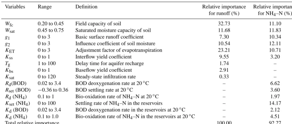
Table 2. Sensitive parameters, their value ranges and relative importance for runoff and NH4–N simulations.
Variables Range Definition Relative importance Relative importance
for runoff (%) for NH4–N (%)
Wfc 0.20 to 0.45 Field capacity of soil 32.73 11.10
Wsat 0.45 to 0.75 Saturated moisture capacity of soil 11.68 11.83
g1 0 to 3 Basic surface runoff coefficient 7.30 10.34
g2 0 to 3 Influence coefficient of soil moisture 10.54 12.11
KET 0 to 3 Adjustment factor of evapotranspiration 23.21 10.71
Kss 0 to 1 Interflow yield coefficient 9.55 3.20
Tg 1 to 100 Delay time for aquifer recharge 1.74 –
Kbs 0 to 1 Baseflow yield coefficient 2.91 –
Ksat 0 to 120 Steady-state infiltration rate 0.33 –
Rd(BOD) 0.02 to 3.4 BOD deoxygenation rate at 20◦C – 6.62
Rset(BOD) −0.36 to 0.36 BOD settling rate at 20◦C – 3.60
Rd(NH4) 0.1 to 1 Bio-oxidation rate of NH4–N at 20◦C – 1.97
Kset(NH4) 0 to 100 Settling rate of NH4–N in the reservoirs – 14.17 Kd(BOD) 0.02 to 3.4 BOD deoxygenation rate in the reservoirs at 20◦C – 2.12 Kd(NH4) 0.1 to 1.0 Bio-oxidation rate of NH4–N in the reservoirs at 20◦C – 4.51
Total relative importance 100.00 92.27
out the consideration of dam regulation. The high and low flows were determined by the cumulative distribution func-tion (CDF). A threshold of 50 % was used for easy presenta-tion; i.e., the flow was treated as high flow (or low flow) if its percentile was greater than (or smaller than) the threshold.
3 Results
3.1 Parameter sensitivity analysis
Nine sensitive parameters were detected for runoff simula-tion by LH-OAT (Table 2), including soil-related parameters
Wfc (field capacity), Wsat(saturated moisture capacity), Kr (interflow yield coefficient) andKsat(steady-state infiltration rate); TVGM parametersg1(basic surface runoff coefficient) andg2(influence coefficient of soil moisture); baseflow pa-rameters Kg(baseflow yield coefficient) andTg(delay time for aquifer recharge); and evapotranspiration parameterKET (adjusted factor of actual evapotranspiration). All of these pa-rameters controlled the main hydrological processes in which soil water and evapotranspiration processes were distinctly important and explained 54.3 and 23.2 % of the runoff varia-tion, respectively.
For NH4–N concentration simulation, over 90 % of ob-served NH4–N concentration variations were explained by 14 sensitive parameters that were categorized into hydrologi-cal (59.28 % of variation), NH4–N (20.65 % of variation) and COD (12.34 % of variation) related parameters. The main ex-planation was that hydrological processes provided the hy-drological boundaries that affected the diffuse source load into rivers and the degradation and settlement processes of NH4–N in water bodies NH4–N concentration was further influenced by the settlement and biological oxidation.
More-over, it was a competitive relationship between COD and NH4–N to consume DO of water bodies in a certain limited level (Brown and Barnwell, 1987).
3.2 Hydrological simulation
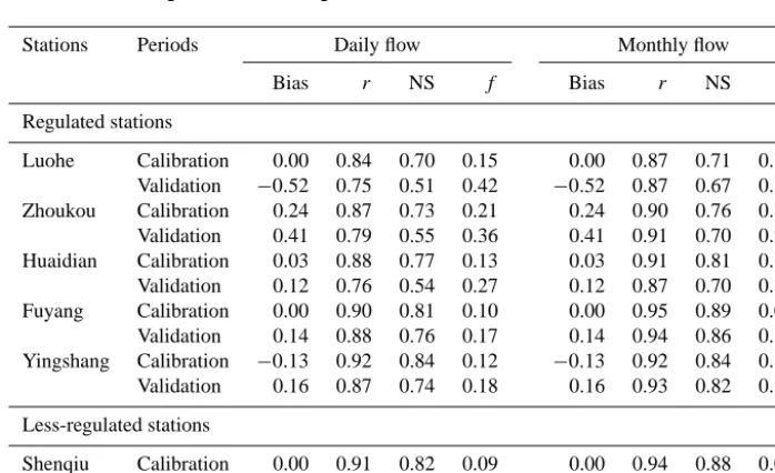
The runoff simulations fitted the observations well at all the stations (Fig. 7 and Table 3). The biases were very close to 0.0 at all the regulated stations except Zhoukou with an un-derestimation (bias: 0.24 for calibration and 0.41 for vali-dation) and Luohe with an overestimation (bias:−0.52 for validation). The obvious biases were caused by the average objective function of all three evaluations rather than the bias only. Ther values ranged from 0.75 (Luohe for validation) to 0.92 (Yingshang for calibration) with the average value of 0.85, whereas the NS values ranged from 0.51 (Luohe for validation) to 0.84 (Yingshang for calibration) with the aver-age value of 0.70. The results of the regulated stations were a little worse than those of the less-regulated station (Shenqiu) owing to the regulation.
Figure 7. The daily runoff simulation at all stations.
Table 3. Runoff simulation results for regulated and less-regulated stations.
Stations Periods Daily flow Monthly flow
Bias r NS f Bias r NS f
Regulated stations
Luohe Calibration 0.00 0.84 0.70 0.15 0.00 0.87 0.71 0.14 Validation −0.52 0.75 0.51 0.42 −0.52 0.87 0.67 0.33 Zhoukou Calibration 0.24 0.87 0.73 0.21 0.24 0.90 0.76 0.19 Validation 0.41 0.79 0.55 0.36 0.41 0.91 0.70 0.26 Huaidian Calibration 0.03 0.88 0.77 0.13 0.03 0.91 0.81 0.10 Validation 0.12 0.76 0.54 0.27 0.12 0.87 0.70 0.18 Fuyang Calibration 0.00 0.90 0.81 0.10 0.00 0.95 0.89 0.05 Validation 0.14 0.88 0.76 0.17 0.14 0.94 0.86 0.11 Yingshang Calibration −0.13 0.92 0.84 0.12 −0.13 0.92 0.84 0.12 Validation 0.16 0.87 0.74 0.18 0.16 0.93 0.82 0.13
Less-regulated stations
Shenqiu Calibration 0.00 0.91 0.82 0.09 0.00 0.94 0.88 0.06 Validation −0.13 0.83 0.67 0.21 −0.13 0.98 0.94 0.08
flow simulations were very obvious. However, their perfor-mances still needed to be improved further, particularly for the underestimation at Zhoukou and Huaidian. The possible reasons were as follows. On the one hand, the applied evalu-ation indices (r and NS) were known to emphasize the high flow simulation rather than the low flow simulation (Push-palatha et al., 2012), and the objective of autocalibration was to obtain the optimal solution for the average of three
evalu-ation indices rather than the bias only. The slight sacrifice of bias improved the overall simulation performance evaluated by all three indices. One the other hand, the dam regulation module still could not fully capture the low flows.
[image:13.612.122.471.381.594.2]542 Y. Y. Zhang et al.: Integrated water system simulation
Figure 8. The cumulative distributions of simulated and observed daily runoff at all stations.
Table 4. The runoff simulation results at regulated stations with and without the dam regulation considered. Range means the difference of the objective function value between regulations considered and not considered. If the range value is less than 0.0, then the simulation with regulation is better than that without regulation. Otherwise, the simulation without regulation is better.
Stations Regulated capacity (%) Flow event Regulation considered Regulation not considered Range
Bias r NS f Bias r NS f
Luohe 0.26 High −0.16 0.97 0.92 0.09 −0.62 0.97 0.80 0.29 −0.20
Low −0.02 0.98 0.69 0.12 −1.46 0.99 −5.53 2.67 −2.55 Average −0.15 0.97 0.93 0.08 −0.68 0.96 0.82 0.30 −0.22
Zhoukou 1.31 High 0.21 0.98 0.93 0.10 −0.38 0.98 0.87 0.18 −0.08
Low 1.00 0.00 −2.57 1.86 −0.64 0.99 −0.08 0.58 1.28 Average 0.30 0.99 0.93 0.13 −0.41 0.98 0.89 0.18 −0.05
Huaidian 1.37 High 0.02 0.98 0.95 0.03 −0.64 0.98 0.68 0.32 −0.29
Low 0.36 0.97 0.43 0.32 −1.51 0.98 −5.88 2.80 −2.48 Average 0.06 0.98 0.96 0.04 −0.74 0.98 0.72 0.35 −0.31
Fuyang 2.21 High 0.04 0.98 0.96 0.03 −0.39 0.99 0.86 0.18 −0.15
Low 0.17 0.99 0.87 0.10 −1.43 0.99 −3.78 2.07 −1.97 Average 0.05 0.99 0.97 0.03 −0.50 0.99 0.88 0.21 −0.18
Yingshang 1.76 High 0.03 0.98 0.95 0.03 −0.44 0.99 0.86 0.20 −0.17
[image:14.612.52.543.499.702.2]Figure 9. The simulated NH4–N concentration variation at all stations.
0.92, whereas the NS values ranged from 0.67 (Luohe for validation) to 0.94 (Shenqiu for validation) with the aver-age value of 0.80. Compared with the existing results at the same stations by SWAT (Zhang et al., 2013), the flow simu-lations at the downstream stations were improved, although they became a little worse at the upstream stations (Luohe and Zhoukou for calibration). In particular, the total water volume and agreements with the observations (i.e., bias and NS) were well captured.
3.3 Water quality simulation
The simulated concentrations of NH4–N matched well with the observations according to the evaluation standard recom-mend by Moriasi et al. (2007) (Fig. 9 and Table 5). Ther val-ues were over 0.60 for all the stations except Zhoukou (0.56 for validation), Yingshang (0.49 for validation) and Shenqiu (0.41 for validation), and the average value was 0.67. The bi-ases were considered to be “acceptable” with a range from −0.27 (Fuyang for validation) to 0.29 (Zhoukou for calibra-tion). The best simulation was at Luohe station. The obvious discrepancies between the simulations and observations of-ten appeared in the period from January to May because of the poor simulation performances on the low flows. Although the biases changed markedly from calibration to validation at Fuyang and Yingshang stations, the model performances were still acceptable. The possible explanation was that the biases for corresponding runoff simulations at these two sta-tions also changed.
Compared with the results without the consideration of regulation, the simulation results were obviously improved
when the regulation was considered, except those at Fuyang station in the calibration period. The decreases in thefNH4−N value ranged from 0.10 (Huaidian for calibration) to 0.49 (Zhoukou for validation), although there was a slight increase at Fuyang for the calibration (0.02). Therefore, it was con-cluded that the consideration of dam and sluice regulation played an important role in the water quality simulation. In the upper stream of the Shaying River, the flow was small and the NH4–N concentration decreased obviously because of the degradation and settlement of large water storage. In the downstream of the Shaying River, the NH4–N concen-tration increased because of the pollutant accumulation and the decreasing flow from dams and sluices owing to the reg-ulation (Zhang et al., 2010). Therefore, the simulated con-centrations without regulation were usually overestimated or higher than the simulation with regulation at the upstream stations (Luohe and Zhoukou). However, the concentrations were underestimated at the downstream stations (Huaidian, Fuyang and Yingshang). The largest differences between the simulations with and without the consideration of regulation appeared at Zhoukou.
544 Y. Y. Zhang et al.: Integrated water system simulation
Table 5. The comparison of NH4–N simulation results with and without dam regulation considered.
Stations Periods Regulated Unregulated Range Ratio of diffuse
Bias r f Bias r f source load (%)
Regulated stations
Luohe Calibration −0.02 0.93 0.05 −0.67 0.60 0.54 −0.49 46.10
Validation – – – – – –
Zhoukou Calibration 0.29 0.61 0.34 −0.56 0.38 0.59 −0.25 44.54 Validation 0.27 0.56 0.36 −1.35 0.66 0.85 −0.49
Huaidian Calibration 0.22 0.73 0.25 0.49 0.80 0.35 −0.10 31.72 Validation 0.02 0.67 0.18 0.22 0.51 0.36 −0.18
Fuyang Calibration 0.28 0.78 0.25 0.26 0.80 0.23 0.02 33.12
Validation −0.27 0.76 0.26 −0.38 0.56 0.41 −0.15
Yingshang Calibration 0.24 0.79 0.23 0.25 0.58 0.34 −0.11 33.26 Validation −0.24 0.49 0.38 −0.76 0.62 0.57 −0.19
Less-regulated stations
Shenqiu Calibration 0.13 0.62 0.26 – – – – 47.13
Validation 0.16 0.41 0.37 – – – –
Figure 11. The spatial pattern of corn yield at the sub-basin and regional scale in the Shaying River catchment.
region was 21.31 % when the two regions with the biggest biases (Fuyang and Pingdingshan) were excluded as outliers. The high load regions were in the middle of the Pingding-shan, Xuchang, Zhengzhou, Fuyang and Zhoukou regions. The spatial pattern was significantly correlated with the dis-tribution of paddy area (r=0.506,p <0.001) and rice yield (r=0.799,p <0.001) (Fig. 10b and c). The fertilizer losses in the paddy areas might be the primary contributor to the dif-fuse source NH4–N load because the average nitrogen loss coefficient in China was just 30–70 % in the paddy areas, which was higher than that in the dryland agriculture (20– 50 %) (Zhu, 2000; Xing and Zhu, 2000).
Summarized from the collected data for model input, the observed average load of point source NH4–N into rivers was approximately 4.70×10⁴t year−1in the Shaying River catch-ment. The diffuse source contributed 38.57 % of the over-all NH4–N load on average from 2003 to 2005, and this value was slightly higher than the statistical results (29.37 %) given in the official report (Wang, 2011). Moreover, the dif-fuse source contributions at the stations ranged from 31.72 % (Huaidian) to 47.13 % (Shenqiu). Compared with the diffuse source loads in the individual administrative regions in 2000, the simulated loads tended to increase from 2003 to 2005, except in the Kaifeng region. The yields in the Fuyang and Pingdingshan regions increased at the highest rates. The pri-mary pollution source in the Shaying River catchment was still the point source, but the diffuse source was also an im-portant concern. In terms of spatial variation, the contribu-tion of diffuse source to the pollutant load was high in the upstream and low in the middle and downstream because the point source emission was usually concentrated in the
mid-dle and downstream. Therefore, compared with the results in Zhang et al. (2013), the overall simulation performance of NH4–N concentration was also improved remarkably by considering the detailed nutrient processes in the soil layers. 3.4 Crop yield simulation
546 Y. Y. Zhang et al.: Integrated water system simulation 4 Discussion
4.1 Comparison with other models
It is a natural tendency that models grow in complexity in order to capture more interactions of complex water-related processes in the real basins because of more and more avail-able observations and improved accuracies (Beven, 2006). Our proposed model was developed in this direction and tended to benefit integrated river basin management, al-though the model applicability needs to be further evaluated in different regions. In comparison with most existing mod-els, our proposed model considered all the water-related pro-cesses as an integrated system rather than isolated systems for individual processes.
Our model provided competitive simulation results in the Huai River basin (Figs. 7–9; Tables 3–5). Several typical models were also applied in this basin, such as SWAT for the monthly runoff and water quality simulation at the reg-ulated stations (Zhang et al., 2013), the SWAT and Xingan-jiang models for the daily runoff simulation at the unregu-lated upstream stations (Shi et al., 2011) and the DTVGM for daily runoff simulation (Ma et al., 2014). Compared with the results of these models, our model generally performed better in the runoff or water quality simulations. In particular, our model performed even better than SWAT at the regulated stations, as more detailed dam regulation rules and soil bio-chemical processes were considered. For example, the aver-age values offrunoffat the monthly scale decreased from 0.32 (SWAT in Zhang et al., 2013) to 0.15 (our model) at the regu-lated stations. The average values offNH4−Ndecreased from 0.47 (SWAT in Zhang et al., 2013) to 0.27 (our model). More-over, both the Xinanjiang model and the DTVGM are lim-ited to simulating the flow series at the unregulated or less-regulated stations because they do not consider the dam reg-ulation in their current model frameworks (Shi et al., 2011; Ma et al., 2014).
4.2 Equifinality
Until now, our understandings of water-related processes have still been ambiguous, and it is hard to describe all these processes in the real-word systems from strong physical foundations (Beven, 2006; Hrachowitz et al., 2014). Empiri-cal equations are usually adopted to approximate the physiEmpiri-cal processes with numerous unknown parameters, especially in the large-scale models. A single output variable of models is associated with multiple processes and many parameters. For examples, SWAT contains over 200 parameters (Arnold et al., 1998) and DNDC has nearly 100 parameters (Li et al., 1992). Pohlert et al. (2006) reported that six hydrolog-ical and 12 N-cycle sensitive parameters were detected in SWAT-N for the simulation of water flow and N leaching. In the case study, 9 and 14 sensitive parameters of our model were detected for runoff and NH4–N simulation, respectively
(Table 2). Therefore, due to the large numbers of model pa-rameters and limited observations, most existing models are subject to equifinality, which is more serious if more water-related processes are considered or more sub-basins are de-lineated for the distributed models.
Several strategies would be helpful to alleviate the equifi-nality, such as field experiments on the physical parameters (Kirchner, 2006), the utilization of more observed processes, multiple evaluation measures for a single predicted compo-nent (Her and Chaubey, 2015), parameter regularization and process constraints (Tonkin and Doherty, 2005; Pokhrel et al., 2008; Euser et al., 2013). Moreover, some attempts are made to move away from traditional curve fitting towards more process consistency and efficient model selection tech-niques (Hrachowitz et al., 2014; Fovet et al., 2015).
For our model, all the independent calibration and valida-tion data sets were specified in Table 1, and most widely used measures of model performances were also provided in the PAT. In the case study, we also employed several observation sources (e.g., runoff and water quality observations at differ-ent stations, the diffuse pollution load and crop yield data) and used three measures to evaluate model performance for the individual components (e.g., bias,r and NS). To make full use of the existing data in practice, parameter sensitivity analysis would be an effective way to reduce dimensional-ity in model calibration and then focus only on the critical processes and parameters that are sensitive to model outputs (van Griensven et al., 2006). Model autocalibration would be efficient to obtain the optimal simulations from numerous samples in multi-dimensional parameter spaces.
4.3 Model limitations
It should be noted that our extended model still has several limitations.
1. The mathematical descriptions of groundwater, crop growth processes and agriculture management practices were still inaccurate. The current version focused on the detailed descriptions of hydrological and nutrient cycles in the soil layers and water bodies, and the consider-ation of dam regulconsider-ation. Satisfactory performances on water quantity and quality simulation were achieved in our case study. However, the simulations for groundwa-ter, diffuse pollution and crop yield in the agriculture regions could be improved further. The stratification of water impounding in the water quality module should be considered if the high-resolution bathymetric data of dams or lakes are available.
nature (Her and Chaubey, 2015). Although the param-eter sensitivity analysis and calibration are widely used to handle the high parameterization issue, the equifinal-ity and parameter uncertainty are still inevitable because of the insufficient observations and the complex interac-tions among different subsystems.
5 Conclusions
In this study, the TVGM hydrological model was extended primarily to an integrated water system model to address the complex water issues emerging in the basins. The model performance was demonstrated in the Shaying River catch-ment, China. The model provided a reasonable tool for the ef-fective water governance by simultaneously simulating sev-eral indicative components of water-related processes includ-ing the hydrological components (e.g., runoff, soil mois-ture, evaporation and plant transpiration, water storage in the dams and sluices), water quality components (e.g., dif-fuse pollution source load, water quality concentrations in water bodies) and ecological components (e.g., crop yield), which could be calibrated if observations were available. The case study showed that the simulated runoffs at most stations fitted the observations well in the highly regulated Shaying River catchment. All the evaluation criteria were acceptable for both the daily and monthly simulations at most stations. This model simulated the discontinuous daily NH4–N con-centration well and properly captured the spatial patterns of diffuse pollution load and corn yield.
548 Y. Y. Zhang et al.: Integrated water system simulation Appendix A: Hydrological cycle module
The basic water balance equation is
Pi+SWi=SWi+1+Rsi+Eai+Rssi+Rbsi+Ini, (A1)
where P is the precipitation (mm); SW is the soil mois-ture (mm);Ea is the actual evapotranspiration (mm) includ-ing soil evaporation (Es, mm) and plant transpiration (Ep, mm); Rs, Rss and Rbs are the surface runoff, interflow and baseflow (mm), respectively; In is the vegetation interception (mm) andiis the time step (day).
Es andEpare determined by the potential evapotranspi-ration (E0, mm), leaf area index (LAI, m2m−2) and surface soil residues (rsd, t ha−1) (Ritchie, 1972) as
Ea=Et+Es≤E0,
Ep=
LAI·E0/3 0≤LAI≤3.0,
E0 LAI>3.0,
Es=E0·exp(−5.0×10⁻⁵×rsd),
(A2)
where E0 is calculated by the Hargreaves method (Harg-reaves and Samani, 1982).
The surface runoff (Rs, mm) yield equation (TVGM; Xia et al., 2005) is given as
Rs=g1(SWu/Wsat)g2·(P−In), (A3) where SWuandWsatare the surface soil moisture and satu-ration moisture (mm), respectively;g1andg2 are the basic coefficient of surface runoff and the influence coefficient of soil moisture, respectively.
The interflow (Rss, mm) and baseflow (Rbs, mm) have linear relationships with the soil moistures in the upper and lower layers, respectively (Wang et al., 2009), as
Rss=kss·SWu, Rbs=kbs·SWl,
(A4) wherekssandkbsare the yield coefficients of interflow and baseflow, respectively; SWlis the soil moisture in the lower layer (mm).
The infiltration from the upper to lower soil layers is calcu-lated using the storage routing method (Neitsch et al., 2011) as
Winf=(SWu−Wfc)· [1−exp(−24/Tinf)],
Tinf=(Wsat−Wfc)/Ksat,
(A5) whereWinf is the water infiltration amount on a given day (mm); Wfc is the soil field capacity (mm); and Tinf is the travel time for infiltration (h), respectively; Ksat is the sat-urated hydraulic conductivity (mm h−1).
The calculation of overland flow routing is adopted from Neitsch et al. (2011) as
Qoverl= Q0overl+Qstor,i−1 ·1−exp(−Tretain/Troute),
Troute=Toverl+Trch=
L0.6overl·n0.6overl
18·slp0.3overl +0.62·Lrch·n
0.75 rch
A0.125·slp0.375 rch
,
(A6)
whereQoverl is the overland flow discharged into the main channel (mm);Q0overlis the lateral flow amount generated in the sub-basin (mm);Qstor,i−1is the lateral flow in the pre-vious day (mm);Tretainis the residence time of flow (days);
Trouteis the flow routing time in sub-basin (days);Toverland
Trch are the routing times of overland flow and river flow, respectively (days);Loverl andLrchare the lengths of sub-basin slope and river, respectively (km); slpoverl and slprch are the slopes of sub-basin and river, respectively (m m−1);
noverl andnrch are the Manning roughness coefficients for sub-basin and river, respectively (m m−1); andAis the sub-basin area (km2).
Appendix B: Soil biochemical module B1 Soil temperature (Williams et al., 1984)
T (Z, t )= ¯T+(AM/2·cos[2π·(t−200)/365]
+TG−T (0, t ))·exp(−Z/DD), (B1) whereZ is the soil depth (mm); t is the time step (days);
¯
T and TG are the average annual temperature and surface temperature (◦C), respectively; AM is the annual variation amplitude of daily temperature; and DD is the damping depth (mm) of soil temperature given as
DD=DP·exp(ln(500/DP)· [(1−ξ )(1+ξ )]2 ,
DP=1000+2500BD/BD+686 exp(−5.63BD), ξ=SW[(0.356−0.144BD)·ZM],
TGIDA=(1−AB)·(Tmx+Tmn) /2·(1−RA/800)
+Tmx·RA/800+AB·TGIDA−1,
(B2)
where DP is the maximum damping depth of soil temperature (mm); BD is the soil bulk density (t m−3);ζis a scale param-eter; IDA is the day of the year; AB is the surface albedo; and RA is the daily solar radiation (ly).
B2 C and N cycle (Li et al., 1992)
Decomposition. The decomposition of resistant and labile C
is described by the first-order kinetic equation, viz.
andk2are the specific decomposition rates of labile faction and resistant fraction, respectively (day−1).
The NH4amount (FIXNH4, kg ha−1) absorbed by clay and organic matter is estimated by
FIXNH4=
0.41−0.47·log(NH4)·(CLAY/CLAYmax) , (B4)
where NH4 is the NH+4 concentration in the soil liquid (g kg−1). CLAY and CLAYmaxare the clay content and the maximum clay content, respectively.
log(KNH4/KH2O)=log(NH4m/NH3m)+pH, NH3m
=10 n
log(NH4)−(log(KNH4)−log(KH2O))+pHo·(CLAY/CLAYmax)
, AM=2·(NH3)·(D·t /3.14)0.5,
(B5)
where KNH4 and KH2O are the dissociation constants for
NH+4 : NH3 equilibrium and H+: OH−equilibrium, respec-tively; NH4m and NH3m are the NH
+
4 and NH3 concentra-tions (mol L−1) in the liquid phase, respectively; AM andD
are the accumulated NH3loss (mol cm−2) and diffusion co-efficients (cm2d−2), respectively.
The nitrification rate (dNNO, kg/ha/day) is a function of the available NH+4, soil temperature and moisture; N2O emis-sion is a function of soil temperature and soil NH+4 concen-tration, and is given as
dNNO=NH4· [1−exp(−K35·µt,n·dt )] ·µSW,n,
N2O=(0.0014·NH4/30.0)·(0.54+0.51·T )/15.8, (B6) whereK35 is the nitrification rate at 35◦C (mg kg−1ha−1);
µSW,nis the soil moisture adjusted factor for nitrification. Denitrification. The growth rate of denitrifiers ((dB/dt )g, kg ha−1day−1) is proportional to their respective biomass and is calculated by the double Monod kinetics equation as
(dB/dt )g=µDN·B(t ),
µDN=µt,dn·(uNO3·µPH,NO3+uNO2·µPH,NO2 +uN2O·µPH,N2O),
uNxOy =uNxOy,max·(C/KC,1/2+C)
·(NxOy/KNxOy,1/2+NxOy),
(B7)
whereB is the denitrifier biomass (kg);µDN is the relative growth rate of the denitrifiers;uNxOy anduNxOy,maxare the
relative and maximum growth rates of NO−2, NO−3 and N2O denitrifiers, respectively.KC,1/2 andKNxOy,1/2are the half
velocity constants of C and NxOy, respectively; µPH,NxOy
and µt,dn are the reduction factors of soil pH and temper-ature, respectively. The mathematical expressions are given as
µPH,NO3=7.14·(pH−3.8)/22.8,
µPH,NO2=1.0,
µPH,N2O=7.22·(pH−4.4)/18.8,
µt,dn=
2(T−22.5)/10 if T <60◦C,
0 if T ≥60◦C.
(B8)
The death rate of denitrifier ((dB/dt )d, kg ha−1h−1) is pro-portional to denitrifier biomass and is given as
(dB/dt )d=MC·YC·B(t ), (B9) where MC and YC are the maintenance coefficient of C (1 h−1) and maximum growth yield of dissolved C (kg ha−1hr−1), respectively.
The consumption rates of dissolved C and CO2production are calculated as
dCcon/dt=(µDN/YC+MC)·B(t )·µSW,d dCO2/dCcon,tdt−(dB/dt )d,
(B10) whereµSW,d is the soil moisture adjusted factor for denitri-fication.
The NO−3, NO−2, NO and N2O consumption is calculated as
dNxOy/dt=(uNxOy/YNxOy+MNxOy·NxOy/N)
·B(t )·µPHNxOy·µt,dn, (B11)
where MNxOy and YNxOy are the maintenance coefficient
(1 h−1) and maximum growth yield on NO−3, NO−2, NO or N2O (kg ha−1h−1), respectively.
N assimilation is calculated on the basis of the growth rates of denitrifiers and the C : N ratio (CNRD:N ) in the bacteria, viz.
(dN/dt )ass=(dB/dt )g·(1/CNRD:N). (B12) The emission rates are the functions of adsorption coeffi-cients of the gases in soils and to the air-filled porosity of the soil, and are given as
P (N2)=0.017+((0.025−0.0013·AD)·PA
P (N2O)= [30.0·(0.0006+0.0013·AD) +(0.013−0.005·AD)] ·PA
P (NO)=0.5· [(0.0006+0.0013·AD)
+(0.013−0.005·AD)·PA]
(B13)
whereP (N2),P(NO) andP (N2O)are the emission rates of N2, NO, and N2O, respectively, during a day; PA and AD are the air-filled fractions of the total porosity and adsorption factor depending on the clay content in the soil, respectively.
Nitrate leaching. The NO−3 leaching rate is a function of clay content, organic C content and water infiltration in the soil layer, and is given as
LeachNO3=Winf·µCLAY·µsoc, (B14)
where LeachNO3 is the NO
−
3 leaching rate;µCLAYandµsoc are the influence coefficients of clay content and soil organic C, respectively.
B3 P cycle
550 Y. Y. Zhang et al.: Integrated water system simulation Appendix C: Dam regulation module (Zhang et al.,
2013)
The water balance model of the dam or sluice is considered the inflow, outflow, precipitation, evapotranspiration, seep-age and water withdrawal. The equation is
1V =Vflowin−Vflowout+Vpcp−Vevap−Vseep−Vwithd, (C1) where 1V,Vflowin andVflowout are the water storage varia-tion, and water volumes of entering and flowing out, respec-tively (m3), and are calculated by HCM;Vpcp,VevapandVseep are the volumes of precipitation, evaporation and seepage, re-spectively (m3), and are the functions of surface water area and water storage.Vwithdis the water withdraw volume (m3) by humans and is given as a model input.
According to the design data of dams and sluices in China, there is a particular relationship among water level, storage and outflow. The outflow is determined by the water level or water storage volume. The relationships are described by equations.
Vflowout=f0(V , H ),
SA=f00(V , H ), (C2)
whereV andH are the water storage volume (m3)and wa-ter level (m) during a day, respectively; f0()andf00() are the functions that could be determined by statistical analy-sis methods (e.g., correlation analyanaly-sis, linear or nonlinear re-gression analysis, polynomial rere-gression analysis and least squares fitting).
Appendix D: Evaluation indices of model performance Bias:
bias= N X
i=1
(Oi−Si)
, N
X
i=1
Oi (D1)
Relative error:
re= N X
i=1
Oi−Si
Oi
×100 % (D2)
Root mean square error:
RMSE= v u u t
N X
i=1
(Oi−Si)2/N (D3)
Correlation coefficient:
r= N X
i=1
(Oi− ¯O)·(Si− ¯S) ,vu
u t N X
i=1
(Oi− ¯O)2· N X
i=1 Si− ¯S
2
(D4)
Nash–Sutcliffe efficiency:
NS=1− N X
i=1
(Oi−Si)2
, N
X
i=1
(Oi− ¯O)2, (D5)
The Supplement related to this article is available online at doi:10.5194/hess-20-529-2016-supplement.
Acknowledgements. This study was supported by the Natural Science Foundation of China (no. 41271005), the China Youth Innovation Promotion Association CAS (no. 2014041), the Pro-gram for “Bingwei” Excellent Talents (no. 2015RC201) and the Key Project for the Strategic Science Plan (no. 2012ZD003) in IGSNRR, CAS, the Endeavour Research Fellowship, the China Visiting Scholar Project from the China Scholarship Council, and the CSIRO Computational and Simulation Sciences Research Platform. The authors would like to thank Yongqiang Zhang and James R. Frankenberger for their participation in our internal review procedure, Markus Hrachowitz and Christian Stamm for improving the quality and presentation of the manuscript, and the anonymous reviewers for their valuable comments and suggestions.
Edited by: M. Hrachowitz
References
Abbott, M. B., Bathurst, J. C., Cunge, J. A., O’Connell, P. E., and Rasmussen, J.: An Introduction to the European System: Systeme Hydrologique Europeen (SHE), J. Hydrol., 87, 61–77, 1986.
Abrahamsen, P. and Hansen, S. D.: an open soil-crop-atmosphere system model, Environ. Model. Softw., 15, 313–330, 2000. Arheimer, B. and Brandt, M.: Modelling nitrogen transport and
re-tention in the catchments of southern Sweden, Ambio, 27, 471– 480, 1998.
Arheimer, B. and Brandt, M.: Watershed modelling of non-point nitrogen pollution from arable land to the Swedish coast in 1985 and 1994, Ecol. Engin., 14, 389–404, 2000.
Arnold, J. G., Srinivasan, R., Muttiah, R. S., and Williams, J. R.: Large-area hydrologic modeling and assessment: Part I. Model development, J. Am. Water Resour. Assoc., 34, 73–89, 1998. Beven, K. J.: A manifesto for the equifinality thesis, J. Hydrol., 320,
18–36, 2006.
Beven, K. J. and Kirkby, M. J.: A physically based variable con-tributing area model of basin hydrology, Hydrol. Sci. Bull., 24, 43–69, 1979.
Bicknell, B. R., Imhoff, J. C., Kittle, J. L., Donigian, A. S., and Johanson, R. C.: Hydrologic Simulation Program – FORTRAN (HSPF): User’s Manual for Release 10, Report No. EPA/600/R– 93/174, US EPA Environmental Research Lab, Athens, Ga, 1993. Borah, D. K. and Bera, M.: Watershed-scale hydrologic and nonpoint-source pollution models: Review of application, Trans. ASAE, 47, 789–803, 2004.
Bouraoui, F. and Dillaha, T. A.: ANSWERS – 2000: Runoff and sediment transport model, J. Environ. Eng., 122, 493–502, 1996. Brown, L. C. and Barnwell, T. O.: The enhanced stream water qual-ity models QUAL2E and QUAL2E-UNCAS: documentation and user manual, Tufts University and Env. Res. Laboratory, US EPA, Athens, Georgia, 1987.
Burt, T. P. and Pinay, G.: Linking hydrology and biogeochemistry in complex landscapes, Prog. Phys. Geog., 29, 297–316, 2005.
China’s national standard (CNS): Current land use condition clas-sification (GB/T21010–2007), General administration of quality supervision, inspection and quarantine of China and Standard-ization administration of China, Beijing, China, 2007.
Deb, K., Pratap, A., Agarwal, S., and Meyarivan, T.: A fast and eli-tist multiobjective genetic algorithm: NSGA–II, IEEE T. Evolut. Comput., 6, 182–197, 2002.
Deng, J., Zhu, B., Zhou, Z. X., Zheng, X. H., Li, C. S., Wang, T., and Tang, J. L.: Modeling nitrogen loadings from agricultural soils in southwest China with modified DNDC, J. Geophys. Res., 116, G02020, doi:10.1029/2010JG001609, 2011.
Di Toro, D. M., Fitzpatrick, J. J., and Thomann, R. V.: Water qual-ity analysis simulation program (WASP) and model verification program (MVP)-Documentation, Hydroscience, Inc., Westwood, NY, for US EPA, Duluth, MN, Contract No. 68–01–3872, 1983. Duan, Q., Sorooshian, S., and Gupta, V. K.: Optimal use of the SCE-UA global optimization method for calibrating watershed mod-els, J. Hydrol., 158, 265–284, 1994.
Efstratiadis, A. and Koutsoyiannis, D.: One decade of multi-objective calibration approaches in hydrological modelling: a re-view, Hydrol. Sci. J., 55, 58–78, 2010.
Euser, T., Winsemius, H. C., Hrachowitz, M., Fenicia, F., Uhlen-brook, S., and Savenije, H. H. G.: A framework to assess the realism of model structures using hydrological signatures, Hy-drol. Earth Syst. Sci., 17, 1893–1912, doi:10.5194/hess-17-1893-2013, 2013.
Fovet, O., Ruiz, L., Hrachowitz, M., Faucheux, M., and Gascuel-Odoux, C.: Hydrological hysteresis and its value for assessing process consistency in catchment conceptual models, Hydrol. Earth Syst. Sci., 19, 105–123, doi:10.5194/hess-19-105-2015, 2015.
Gassman, P. W., Reyes, M. R., Green, C. H., and Arnold, A. G.: The soil and water assessment tool: historical development, applica-tions, and future research direcapplica-tions, T. ASABE, 50, 1211–1250, 2007.
Goldberg, D. E.: Genetic algorithms in search, optimization, and machine learning, Reading Menlo Park: Addison-Wesley, Mas-sachusetts, USA, 1989.
Hamrick, J. M.: A three-dimensional environmental fluid dynamics computer code: theoretical and computational aspects, Special Report, The College of William and Mary, Virginia Institute of Marine Science, Virginia, USA, 317, 1992.
Hargreaves, G. H. and Samani, Z. A.: Estimating potential evapo-transpiration, J. Irrigat. Drain. Div., 108, 225–230, 1982. Henan Statistical Yearbook in 2003, 2004 and 2005: China Statistics
Press, Beijing, 2003, 2004, 2005.
Her, Y. and Chaubey, I.: Impact of the numbers of observations and calibration parameters on equifinality, model performance, and output and parameter uncertainty, Hydrol. Process., 29, 4220– 4237, 2015.
Horst, W. J., Kamh, M., Jibrin, J. M., and Chude, V. O.: Agronomic measures for increasing P availability to crops, Plant. Soil., 237, 211–223, 2001.