https://doi.org/10.5194/hess-22-3739-2018 © Author(s) 2018. This work is distributed under the Creative Commons Attribution 4.0 License.
Transferability of climate simulation uncertainty to
hydrological impacts
Hui-Min Wang1, Jie Chen1, Alex J. Cannon2, Chong-Yu Xu1,3, and Hua Chen1
1State Key Laboratory of Water Resources and Hydropower Engineering Science, Wuhan University,
Wuhan, 430072, China
2Climate Research Division, Environment and Climate Change Canada, Victoria BC, Canada 3Department of Geosciences, University of Oslo, Oslo, Norway
Correspondence:Jie Chen ([email protected])
Received: 30 November 2017 – Discussion started: 2 January 2018 Revised: 1 June 2018 – Accepted: 4 June 2018 – Published: 16 July 2018
Abstract.Considering rapid increases in the number of cli-mate model simulations being produced by modelling cen-tres, it is often infeasible to use all of them in climate change impact studies. In order to thoughtfully select subsets of cli-mate simulations from a large ensemble, several envelope-based methods have been proposed. The subsets are expected to cover a similar uncertainty envelope to the full ensemble in terms of climate variables. However, it is not a given that the uncertainty in hydrological impacts will be similarly well represented. Therefore, this study investigates the transfer-ability of climate uncertainty related to the choice of climate simulations to hydrological impacts. Two envelope-based se-lection methods,Kmeans clustering and the Katsavounidis– Kuo–Zhang (KKZ) method, are used to select subsets from an ensemble of 50 climate simulations over two watersheds with very different climates using 31 precipitation and tem-perature variables. Transferability is evaluated by comparing uncertainty coverage between climate variables and 17 hy-drological variables simulated by a hyhy-drological model. The importance of choosing climate variables properly when se-lecting subsets is investigated by including and excluding temperature variables. Results show that KKZ performs bet-ter thanKmeans at selecting subsets of climate simulations for hydrological impacts, and the uncertainty coverage of cli-mate variables is similar to that of hydrological variables. The subset of the first 10 simulations covers over 85 % of total uncertainty. As expected, temperature variables are im-portant for the snow-related watershed, but less imim-portant for the rainfall-driven watershed. Overall, envelope-based selec-tion of around 10 climate simulaselec-tions, based on climate
vari-ables that characterize the physical processes controlling the hydrology of the watershed, is recommended for hydrologi-cal impact studies.
1 Introduction
In studies of climate change impacts on hydrology, multi-model ensembles (MMEs) formed by multiple global cli-mate models (GCMs) and multiple emission scenarios have been widely used to drive hydrological models (Minville et al., 2008; Vaze and Teng, 2011; Chiew et al., 2009; Chen et al., 2011b). There are two strengths of using MMEs: (1) the MME mean typically performs better than any individual model in representing the mean of historical climate observa-tions (Gleckler et al., 2008; Pierce et al., 2009; Pincus et al., 2008; Mehran et al., 2014); and (2) the spread of a MME can be used to estimate climate change impact uncertainties, for example those related to GCM structure, future greenhouse gas concentrations, and internal climate variability (Mend-lik and Gobiet, 2016; Knutti et al., 2010; Chen et al., 2011b; Tebaldi and Knutti, 2007). While climate projection uncer-tainty and spread or coverage of a MME are not equivalent, the latter does provide an imperfect estimate of uncertainty and, for sake of simplicity, we use the terms interchangeably in the remainder of this study.
outputs from 61 GCMs (https://pcmdi.llnl.gov, last access: 19 June 2018), with each GCM contributing one or more simulation runs (Taylor et al., 2012). Although it is usually advised that as many climate simulations as possible be used in impact studies, the extraction, storage, and computational costs associated with a large MME may be prohibitive. In practice, it is not uncommon for impact studies to instead rely on a small subset of climate simulations, which are of-ten selected manually, relying on expert judgement.
Several studies have considered more objective means of selecting subsets of climate simulations for impact studies based on different criteria. Generally, there are two main types of selection approaches. The past-performance ap-proach selects a subset by weighting or selecting simulations according to their ability to represent the observed near-past climate (Gleckler et al., 2008; Perkins et al., 2007; Pincus et al., 2008). Climate model performance is generally evaluated based on agreement with observed climate conditions, which is often defined by a suite of climate metrics. For example, Perkins et al. (2007) ranked climate models based on proba-bility density functions of observed temperature and precip-itation. Similarly, Gleckler et al. (2008) evaluated the per-formances of 22 GCMs according to relative errors of some climatological fields, but stressed that a wider range of met-rics might give more robust results. In general, the assump-tion that models with good performance over the near-past provide more realistic climate change signals is questionable (Knutti et al., 2010; Reifen and Toumi, 2009), although re-cent work on emergent constraints suggests that it may be possible to remove models that fail to represent certain key physical processes that dictate the evolution of long-term cli-mate projections (Klein and Hall, 2015). In practice, how-ever, the metrics commonly used to evaluate model perfor-mance are often manually defined based on the fields of inter-est, which leads to substantial subjectivity within the weight-ing process.
Another means of selecting climate simulations is the envelope-based approach, which tries to select a represen-tative subset of climate simulations that covers as much of the full ensemble’s range of future climate change signals as possible (Warszawski et al., 2014; Cannon, 2015; Logan et al., 2011). For instance, Cannon (2015) used two automated multivariate statistical algorithms, K means clustering and the Katsavounidis–Kuo–Zhang (KKZ) method (Katsavouni-dis et al., 1994), to select subsets of CMIP5 GCMs that bracket the overall range of changes in a suite of 27 climate extreme indices. The goal of the envelope-based approach coincides with the motivation behind the usage of a MME, namely to account for different sources of projection uncer-tainty, including structural uncertainty (Wilcke and Bärring, 2016; Tebaldi and Knutti, 2007).
Some studies have proposed selection methods that com-bine both near-past performance and climate change en-velope coverage criteria (McSweeney et al., 2012; Lutz et al., 2016a; Giorgi and Mearns, 2002). For example, Lutz et
al. (2016a) took both model historical skill and the range of projected changes in means and extremes into consideration through a three-step sequential selection procedure. Since many examples of such selection methods place emphasis on ranking or weighting climate model performance, they may inherit the potential flaws of the past-performance approach. Regardless of underlying approaches, most selection methods are only conducted on climate variables that can be calculated directly from the MME simulation outputs. Even though subsets of simulations that account for most of the ensemble spread in climate variables can be identified, it is not guaranteed that the same level of spread coverage ex-tends to hydrological impact variables due to the complex-ity and non-linearcomplex-ity of hydrological processes. For example, small perturbations in the frequency or intensity of tempera-ture and precipitation regimes may have noticeable impacts on streamflow patterns and flood magnitudes (Muzik, 2001; Whitfield and Cannon, 2000). Consequently, whether the ad-equate coverage of climate simulation uncertainty is trans-ferable to hydrological impacts should be evaluated before applying envelope-based selection methods in hydrological impact studies.
Chen et al. (2016) investigated the transferability of op-timally selected climate simulations in the uncertainty quan-tification of hydrological impacts over a Canadian watershed. They concluded that the transferability of climate simulation uncertainty is limited to hydrological impacts. However, the selection methods used in their study were applied to just two climate variables, mean annual temperature and mean an-nual precipitation, which is a common strategy employed by practitioners who employ envelope-based approaches (Im-merzeel et al., 2013; Warszawski et al., 2014). Hydrological responses are driven both by annual climate conditions and intra-annual climate processes, which may not be described by a small number of climate variables. The transferability of climate uncertainty may be diminished due to insufficient climate variables.
Figure 1.Location maps of the(a)Xiangjiang and(b)Manicouagan 5 watersheds. (The study area in the Xiangjiang watershed is one of its sub-basins, as the orange boundary shows.)
2 Study area and data 2.1 Study area
This study was conducted over two watersheds (the Xi-angjiang and Manicouagan 5 watersheds) with different climate and hydrological characteristics (Fig. 1). The Xi-angjiang watershed is a monsoon-climate and rainfall-dominated watershed located in southern central China, whereas Manicouagan 5 is a temperate-climate and sea-sonally snow-covered watershed located in central Quebec, Canada.
2.1.1 Xiangjiang watershed
The Xiangjiang watershed is one of the largest sub-basins of the Yangtze River watershed (Fig. 1a). The Xiangjiang River originates from the Haiyang Mountains in the Guangxi Au-tonomous Region and flows north to Dongting Lake in Hu-nan Province, which connects to the Yangtze River. The Xi-angjiang River consists of several tributaries with a surface area of approximately 94 660 km2, but only the catchment with an area of 52 150 km2above the Hengyang gauging sta-tion was used in this study. The catchment has a hilly topog-raphy ranging from a maximum elevation of 2042 m a.s.l. to a minimum elevation of 58 m a.s.l. at the Hengyang sta-tion. The Xiangjiang watershed is heavily influenced by a subtropical monsoon climate with hot and humid summers and mild and dry winters. The average annual precipita-tion over the catchment is about 1570 mm almost entirely in the form of rainfall. Around 61 % precipitation occurs from April to August, resulting in high flows during this period. The average daily maximum and minimum temperatures are around 22 and 15◦C, respectively. The average daily dis-charge at the Hengyang station is around 1400 m3s−1. The peak discharge of the averaged daily hydrograph is about 4420 m3s−1, mainly resulting from high-intensity rainfall.
2.1.2 Manicouagan 5 watershed
The Manicouagan 5 watershed, the largest sub-basin of the Manicouagan River watershed, is located in the centre of the province of Quebec, Canada (Fig. 1b). The Man-icouagan 5 River discharges into the ManMan-icouagan reser-voir, an annular reservoir within the remnant of an an-cient eroded impact crater, and ends at the Daniel John-son Dam, which is the largest buttressed multiple arc dam in the world. The drainage area of the Manicouagan 5 River is about 24 610 km2, which is mostly covered by for-est and has a moderately hilly topography ranging from a maximum elevation of 952 m a.s.l. to a minimum ele-vation of 350 m a.s.l. (Chen et al., 2016). The Manicoua-gan 5 watershed has a continental subarctic climate domi-nated by long and cold winters. The annual precipitation is fairly evenly distributed within the year and averages about 912 mm, around 45 % of which is snowfall. The average daily maximum and minimum temperatures are around 2.4 and−7.8◦C, respectively. The average discharge of the Man-icouagan 5 River is about 530 m3s−1. The peak discharge of the averaged daily hydrograph is around 2200 m3s−1, mainly resulting from snowmelt.
2.2 Data
Both observed and simulated daily meteorological (maxi-mum and mini(maxi-mum temperatures and precipitation) data over both watersheds were used in this study. All the climate data from multiple stations or grids were averaged over the water-sheds.
2.2.1 Climate simulations
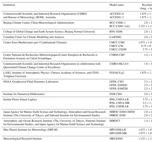
insti-Table 1.Basic information about the CMIP5 models.
Institution Model name Resolution
(long.×lat.) Commonwealth Scientific and Industrial Research Organization (CSIRO) ACCESS1.0 1.875×1.25 and Bureau of Meteorology (BOM), Australia ACCESS1.3 1.875×1.25 Beijing Climate Center, China Meteorological Administration BCC-CSM1.1 2.8×2.8 BCC-CSM1.1(m) 1.125×1.125 College of Global Change and Earth System Science, Beijing Normal University BNU-ESM 2.8×2.8 Canadian Centre for Climate Modelling and Analysis CanESM2 2.8×2.8 Centro Euro-Mediterraneo per I Cambiamenti Climatici CMCC-CMS 1.875×1.875 CMCC-CM 0.75×0.75 CMCC-CESM 3.75×3.7 Centre National de Recherches Météorologiques/Centre Européen de Recherche et
Formation Avancée en Calcul Scientifique
CNRM-CM5 1.4×1.4
Commonwealth Scientific and Industrial Research Organization in collaboration with Queensland Climate Change Centre of Excellence
CSIRO-Mk3.6.0 1.8×1.8
LASG, Institute of Atmospheric Physics, Chinese Academy of Sciences; and CESS, Tsinghua University
FGOALS-g2 1.875×1.25
NOAA Geophysical Fluid Dynamics Laboratory GFDL-CM3 2.5×2.0 GFDL-ESM2G 2.5×2.0 GFDL-ESM2M 2.5×2.0 Institute for Numerical Mathematics INM-CM4 2.0×1.5 Institut Pierre-Simon Laplace IPSL-CM5A-LR 3.75×1.9 IPSL-CM5A-MR 2.5×1.25 IPSL-CM5B-LR 3.75×1.9 Japan Agency for Marine-Earth Science and Technology, Atmosphere and Ocean Research MIROC-ESM-CHEM 2.8×2.8 Institute (The University of Tokyo), and National Institute for Environmental Studies MIROC-ESM 2.8×2.8 Atmosphere and Ocean Research Institute (The University of Tokyo), National Institute
for Environmental Studies, and Japan Agency for Marine-Earth Science and Technology
MIROC5 1.4×1.4
Max Planck Institute for Meteorology (MPI-M) MPI-ESM-LR 1.875×1.875 MPI-ESM-MR 1.875×1.875 Meteorological Research Institute MRI-ESM1 1.125×1.125 MRI-CGCM3 1.1×1.1
tutions were employed to represent climate modelling uncer-tainty (Table 1). Two Representative Concentration Pathways (RCP4.5 and RCP8.5) were used for each GCM to represent forcing scenario uncertainty, with the exception of CMCC-CESM, which only used RCP8.5, and MRI-ESM1, which only used RCP4.5. Only the first run of each GCM was used. On the whole, an ensemble of 50 climate simulations was used in this study.
2.2.2 Observations
Observed daily meteorological data used to downscale the GCM outputs and calibrate the hydrological model cover the 1975–2004 period for both watersheds. Meteorological data
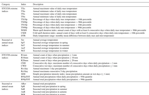
[image:4.612.50.543.79.534.2]Table 2.Definitions of 31 climate variables. The final column indicates whether the change in a given variable is expressed in the form of relative difference (CT: change type).
Category Index Description CT
ETCCDI extreme TXx Annual maximum value of daily max temperature indices TXn Annual minimum value of daily max temperature TNx Annual maximum value of daily min temperature TNn Annual minimum value of daily min temperature
TX10p Percentage of days when daily max temperature<10th percentile TX90p Percentage of days when daily max temperature>90th percentile TN10p Percentage of days when daily min temperature<10th percentile TN90p Percentage of days when daily min temperature>90th percentile
WSDI Warm spell duration index: annual count of days with at least 6 consecutive days when daily max temperature>90th percentile CSDI Cold spell duration index: annual count of days with at least 6 consecutive days when daily min temperature<10th percentile DTR Daily temperature range: monthly mean difference between daily max and min temperature
Seasonal or Tav Annual average temperature annual mean SpT Seasonal average temperature in spring indices SuT Seasonal average temperature in summer
AuT Seasonal average temperature in autumn WiT Seasonal average temperature in winter
ETCCDI extreme R1mm Annual count of days when precipitation≥1 mm indices R10mm Annual count of days when precipitation≥10 mm
R20mm Annual count of days when precipitation≥20 mm
CDD Consecutive dry days: maximum number of consecutive days when daily precipitation<1 mm CWD Consecutive wet days: maximum number of consecutive days when daily precipitation≥1 mm
Rx1day Annual maximum 1-day precipitation % Rx5day Annual maximum consecutive 5-day precipitation % SDII Simple precipitation intensity index: mean precipitation amount on wet days (≥1 mm) % R95pTOT Annual total precipitation when daily precipitation>95th quantile % R99pTOT Annual total precipitation when daily precipitation>99th quantile % Seasonal or ARav Annual total precipitation % annual mean SpR Seasonal total precipitation in spring % indices SuR Seasonal total precipitation in summer % AuR Seasonal total precipitation in autumn % WiR Seasonal total precipitation in winter %
3 Methodology
3.1 Subset selection of GCM simulations
Two automated envelope-based methods were used to select subsets of climate simulations. One is theK means cluster-ing which finds cluster centroids that best characterize high-density regions of a multivariate space; the other is the KKZ method which recursively selects simulations that best span the spread of an ensemble (Cannon, 2015). Both selection methods operate on multivariate data, which means that they are sensitive to the choice and scaling of climate variables.
3.1.1 Climate variables
Since the hydrological response of a watershed not only de-pends on annual mean temperature and precipitation but is also sensitive to intra-annual climate variability (e.g. sea-sonal means or extremes), subset selection should be based on a set of climate variables that includes annual and sea-sonal means as well as extremes. The World Meteorologi-cal Organization’s Expert Team on Climate Change Detec-tion and Indices (ETCCDI) has recommended a set of core climate indices that can be easily derived from daily meteo-rological data series (http://etccdi.pacificclimate.org/list_27_
indices.shtml, last access: 19 June 2018). The ETCCDI in-dices are designed to monitor changes in the frequency and intensity of climate extreme events and characterize the vari-ability of extremes (Zhang et al., 2011). Here, we assume that the ETCCDI indices are sufficient to characterize climate ex-tremes that lead to hydrological impacts.
3.1.2 Kmeans clustering
The Kmeans clustering algorithm divided the ensemble of 50 climate simulations into a user-specified number of clus-ters based on the objective of minimizing within-cluster sum of squared error (SSE) (Hartigan and Wong, 1979). Each cluster is represented by its centroid. The SSE is character-ized by the Euclidean distances from simulations to their cor-responding cluster centroids. Some studies have applied this method to select subsets of climate simulations (Logan et al., 2011; Cannon, 2015; Houle et al., 2012). The climate simu-lations closest to the centroids were selected as the subsets. Due to sensitivity of the Kmeans clustering to initial clus-ter centroid positions, it was run 10 000 times with different initializations and the best solution with the lowest SSE was kept. A disadvantage of the K means clustering is that the selected climate simulations are not ordered. In other words, the selected simulations in a small subset may not be in a larger subset, which means that it is inconvenient for end-users to change the subset size for different applications. 3.1.3 KKZ method
The KKZ method was originally designed by Katsavounidis et al. (1994) to identify a set of optimal seed cases as initial centroids in theK means clustering, and was introduced by Cannon (2015) to the selection of climate simulations. This method prefers the peripheral simulations in the multivariate space. The specific procedure is as follows.
1. The climate simulation closest to the centroid of the whole ensemble is selected as the first simulation. 2. The simulation farthest from the first selected
simula-tion is selected as the second simulasimula-tion. 3. Subsequent simulations are selected as follows.
– For each remaining simulation, its distances to ev-ery previously selected simulation are calculated. – Each remaining simulation is designated with the
minimum distance among all distances calculated in step 3(1).
– The simulation with the largest minimum distance, which is designated in step 3(2), is selected as the next selected simulation.
Compared to the K means clustering, the KKZ method is deterministic and ordered. However, it is more susceptible to selecting outliers thanKmeans clustering. In addition, a random selection, repeated 100 times to minimize the influ-ence of its stochastic nature, was conducted as a baseline to evaluate theKmeans clustering and KKZ method.
3.2 Generation of climate scenarios
GCM outputs are typically on a coarse spatial grid and con-tain systematic biases that preclude their direct use in
hy-drological modelling (Mpelasoka and Chiew, 2009; Chen et al., 2011a, b; Minville et al., 2008; Vaze and Teng, 2011). It is thus necessary to bias correct and downscale GCM out-puts before running the hydrological model. The main objec-tive of this study is to investigate the transferability of cli-mate simulation uncertainty; hence, there is no need to use a complicated downscaling method. A commonly used change factor method, namely the daily scaling (DS) method pro-posed by Harrold and Jones (2003), was used in this study. This method assumes that climate change signals simulated by GCMs are credible and can be used to perturb observa-tions to obtain future daily series. The DS method adjusts the observed daily series using the differences in distributions of simulated temperature/precipitation between the future pe-riod and the reference pepe-riod. The specific steps are the fol-lowing.
1. Distributions (represented by 100 quantiles in this study) of daily temperature and precipitation simulated by GCMs are calculated for both reference and future periods in each calendar month (i.e. January, February, etc.);
2. scaling factors are estimated as the differences (for tem-peratures) or ratios (for precipitation) in distributions of temperature and precipitation between reference and fu-ture periods for each calendar month; and
3. scaling factors are added (for temperatures) or multi-plied (for precipitation) to corresponding distributions of observed daily temperature or precipitation for each calendar month.
The use of the DS method preserves the simulated climate change signal. It is based on differences in probability distri-butions between the reference and future periods, which are only caused by climate change signals. In addition, the con-sideration of quantile-dependent changes in the precipitation distribution is important in hydrological impact studies, be-cause more runoff is generated in high-intensity precipitation events (Harrold and Jones, 2003; Chiew et al., 2009). The use of 100 quantiles in the DS method is the same as many other studies (Mpelasoka and Chiew, 2009; Chen et al., 2013). La-fon et al. (2013) showed that the empirical quantile mapping method based on 100 quantiles is more accurate than that based on 25, 50, or 75 quantiles. However, temporal sequenc-ing in the future period is assumed to be the same as in the observed data. Changes in, for example, wet/dry spell lengths are not informed by the GCM simulations.
3.3 Hydrological response simulation 3.3.1 Hydrological modelling
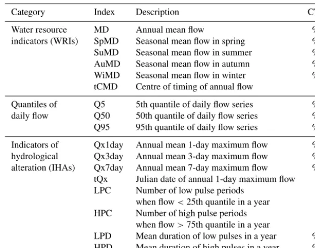
Table 3.Definitions of 17 hydrological variables. The final column indicates whether the change in a given variable is expressed in the form of relative difference (CT: change type).
Category Index Description CT Water resource MD Annual mean flow % indicators (WRIs) SpMD Seasonal mean flow in spring % SuMD Seasonal mean flow in summer % AuMD Seasonal mean flow in autumn % WiMD Seasonal mean flow in winter % tCMD Centre of timing of annual flow
Quantiles of Q5 5th quantile of daily flow series % daily flow Q50 50th quantile of daily flow series % Q95 95th quantile of daily flow series % Indicators of Qx1day Annual mean 1-day maximum flow % hydrological Qx3day Annual mean 3-day maximum flow % alteration (IHAs) Qx7day Annual mean 7-day maximum flow %
tQx Julian date of annual 1-day maximum flow LPC Number of low pulse periods
when flow<25th quantile in a year HPC Number of high pulse periods
when flow>75th quantile in a year
LPD Mean duration of low pulses in a year % HPD Mean duration of high pulses in a year %
CemaNeige snow accumulation and melt routines (Arsenault et al., 2015). The GR4J model is a reservoir-based four-parameter model developed on the basis of the GR3J model (Edijatno et al., 1999; Perrin et al., 2003). This model routes runoff through a production reservoir, two linear unit hy-drographs and a non-linear routing reservoir. Four parame-ters have to be calibrated for this model. They are maximum capacity of the production reservoir, groundwater exchange coefficient, 1-day-ahead maximum capacity of the routine reservoir and time base of unit hydrograph. In an evaluation of the model, Perrin et al. (2003) found that GR4J outper-formed 19 models over a large sample of catchments.
Due to its lack of snow accumulation and snowmelt al-gorithms, the GR4J model cannot be directly used in snow-related watersheds. Thus, the general snow accounting rou-tine proposed by Valéry et al. (2014), CemaNeige, was added. In this routine, precipitation is divided into rainfall and snowfall depending on the daily range of temperatures, and the updating of snowpack and snowmelt is based on a degree-day approach that is controlled by two free parame-ters (cold content factor and snowmelt factor). In addition, the Oudin formulation (Oudin et al., 2005) was used to pre-process evapotranspiration for GR4J-6.
3.3.2 Hydrological variables
To examine the performance of subset selection in terms of hydrological response uncertainty, this study used a set of 17 hydrological variables based on water resource indica-tors (WRIs), indicaindica-tors of hydrologic alteration (IHAs), and
quantiles of daily flow series (Table 3). WRIs have been used in many hydrological impact studies to assess stream-flow alteration due to natural and anthropogenic climate change (Eum et al., 2017; Shrestha et al., 2014; Chen et al., 2011b). IHAs are used to examine the temporal variation of key streamflow hydrograph components (Eum et al., 2017; Richter et al., 1996; Shrestha et al., 2014). Quantiles of daily flow series have been used to describe the characteristics of flow regimes (Mu et al., 2007; Wilby, 2005).
Similar to climate variables, changes in hydrological vari-ables between the reference (1975–2004) and future (2070– 2099) periods were calculated. To remove the influence of systematic biases between the observations and simulations, simulated runoff values instead of gauge observations were used as flow data in the reference period. The first year of each period was used to spin up the hydrological model and was excluded when calculating the hydrological variables. Once the projected changes in hydrological variables were calculated, the uncertainty coverage of subsets could be com-pared between climate variables and hydrological variables to evaluate the transferability of climate simulation uncer-tainty.
3.4 Data analysis
sim-Figure 2.Examples of PSCs when selecting five climate simulations over the Xiangjiang watershed using the KKZ method. The PSCs of each variable are presented beside the corresponding axes.
ulations. A higher PSC means that the selected subset cov-ers a larger uncertainty range. Figure 2 shows examples of PSC when five climate simulations are selected using the KKZ method. Since it is difficult to illustrate results in more than three dimensions, examples are limited to one, two, and three variables. In Fig. 2a, points represent the changes in “WiT” (seasonal average temperature in winter) for 50 GCM simulations. The larger squares represent the same variable for a subset of five climate simulations selected by KKZ. The PSC is calculated by dividing the temperature range of the selected subset, 4.15◦C, by that of the whole ensemble, 6.49◦C. Therefore, for this specific variable the PSC (uncer-tainty coverage) of the subset is 64.01 %. Similarly, every variable has a corresponding PSC associated with a subset of a given size; examples of “WiR” (seasonal total precipitation in winter) and “Rx1day” (annual maximum 1-day precipita-tion) are shown in Fig. 2b–c. For the random subset selection method, the reported PSC is the mean value of 100 PSCs, each calculated for a different random subset of the specified size.
4 Results
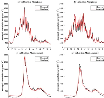
[image:8.612.98.498.70.301.2]Figure 3.Observed and simulated mean hydrographs for(a, c)calibration and(b, d)validation periods over the(a, b)Xiangjiang and
(c, d)Manicouagan 5 watersheds.
Table 4.Nash–Sutcliffe efficiency (NSE) and relative error (RE) of hydrological models in the calibration and validation over two watersheds.
Country Watershed Area Hydrological Calibration NSE RE Validation NSE RE name (km2) model period calibration calibration period validation validation
China Xiangjiang 52 150 GR4J-6 1975–1987 0.912 −0.3 % 1988–2000 0.871 5.4 % GR4J 1975–1987 0.912 −0.2 % 1988–2000 0.872 5.5 %
Canada Manicouagan 5 24 610 GR4J-6 1970–1979 0.926 3.8 % 1980–1989 0.881 2.7 %
4.2 Transferability of climate uncertainty
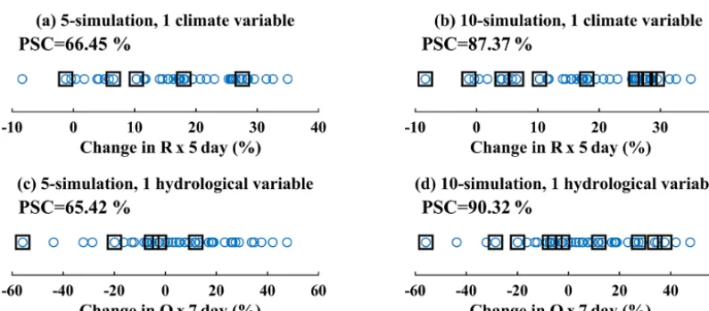
As an illustrative example, the uncertainty transferability from one climate variable to one hydrological variable in the Xiangjiang watershed is shown in Fig. 4. The larger squares represent the 5- and 10-climate simulation subsets selected by the KKZ method. The subfigures on the top dis-play the PSC for “Rx5day” (maximum consecutive 5-day precipitation), whereas those at the bottom display the PSC for “Qx7day” (7-day maximum flow). The reason for choos-ing these two variables is that there is a generally accepted linkage between high-intensity precipitation and high flow in a rainfall-driven watershed. Although this particular choice of climate and hydrological variables is, in some ways,
un-fair because the overall selection process is based on a high-dimensional multivariate climate space, these subfigures still illustrate the process of uncertainty transferability from cli-mate simulations to hydrological impacts. Here, the PSC of the climate variable increases from 66.45 to 87.37 % as the number of selected simulations goes from 5 to 10; at the same time, the PSC of the hydrological variable increases from 65.42 to 90.32 %. In this case, the uncertainty coverage of the subsets in terms of the climate variable is well translated to uncertainty coverage of the hydrological variable.
[image:9.612.49.546.453.526.2](maxi-Figure 4.Examples of the transferability of climate uncertainty to hydrological impacts based on one variable when selecting(a, c)5 and
(b, d)10 climate simulations over the Xiangjiang watershed using the KKZ method. The PSCs of each variable are presented in the top left corner.
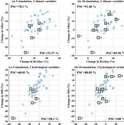
mum 1-day precipitation), whereas those at the bottom show changes in two hydrological variables, “MD” (annual mean flow) and “HPD” (mean duration of high pulses). It should be noted that the subsets of climate simulations are the same as in the 1-D example above. As the number of selected sim-ulations increases from 5 to 10, the mean PSC for the two climate variables increases from 50.83 to 88.72 %, while the mean PSC for the two hydrological variables increases from 59.46 to 94.05 %. The increases are mostly due to selection of outlying simulations in the top right corner of the plots (the sixth, eighth, and ninth selected simulations). There is strong consistency between locations of selected simulations in 2-D climate space and hydrology space. For example, the first, fourth, and tenth selected simulations are close to each other in both climate space (Fig. 5b) and hydrology space (Fig. 5d). Accordingly, the uncertainty coverage tends to translate well from climate variables to hydrological variables in this 2-D example. However, PSC increases are not consistent in all cases. For example, selection of the simulation on the left edge of Fig. 5b (the seventh selected simulation) substan-tially improves the PSC of “Rx1day”, but it does not lie on the edge of Fig. 5d and hence does not contribute to improve-ments in PSC of either hydrology variable. This may be due to the non-linearity of the hydrological model or an imperfect explanatory relationship between the climate and hydrologi-cal variables.
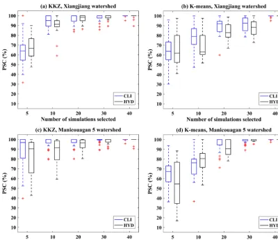
The discussion above is limited to results for 5- and 10-simulation subsets for one watershed selected using the KKZ method. In the study as a whole, subset sizes from 1 to 50 simulations were evaluated in terms of transferability for two watersheds and two envelope-based methods, and PSCs for all 31 climate variables and 17 hydrological variables were calculated. Figure 6 shows distributions of climate and hy-drological PSCs for 5-, 10-, 20-, 30-, and 40-simulation sub-sets. For the Xiangjiang watershed (Fig. 6a–b), PSCs for
the climate variables are similar to those for the hydrologi-cal variables. For the Manicouagan 5 watershed (Fig. 6c–d), PSCs for the hydrological variables are slightly smaller than those for the climate variables. Overall, the tendency of the hydrological PSCs to increase with subset size is compara-ble to that of the climate PSCs in both watersheds. In other words, as the size of a subset becomes larger, the improve-ment in PSCs of the hydrological variables is similar to that of the climate variables. When comparing the two envelope-based methods, KKZ tends to outperformK means cluster-ing.
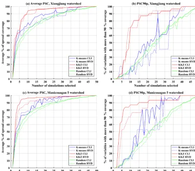
Given the large number of climate and hydrological vari-ables under consideration and the challenges inherent in communicating information about multi-dimensional data, two summary criteria were used to generalize subset cover-age results in this study. The first criterion is the avercover-age PSC for all climate or hydrological variables. Following Cannon (2015), the second criterion is the percentage of variables that reach a 90 % PSC threshold (PSC90p).
[image:10.612.101.499.61.235.2]Figure 5.Examples of the transferability of climate uncertainty to hydrological impacts based on two variables when selecting(a, c)5 and
(b, d)10 climate simulations over the Xiangjiang watershed using the KKZ method. The PSCs of each variable are presented beside the corresponding axes.
for the hydrological variables in some cases (e.g.K=27 to 32). In the case of the Manicouagan 5 watershed (Fig. 7c), the KKZ method again outperformsKmeans clustering and random selection.
In addition, as more simulations are selected, the average PSC increases rapidly when the size of selected simulations is smaller than 10 for both watersheds, while the rate of in-crease slows when the number is larger than 10. For the KKZ method, a subset of 10 simulations covers more than 85 % of uncertainty for climate and hydrology variables in both wa-tersheds; selecting more than 10 climate simulations leads to little change in uncertainty coverage. For both watersheds, a subset of 10 simulations selected by KKZ appears to be optimal for reducing computational costs while incurring the smallest possible loss of uncertainty information. In addition,
the performance of the KKZ method is maintained for larger subsets, while the performance ofKmeans clustering fluctu-ates. In other words, a larger subset selected by theKmeans clustering may not have a greater uncertainty coverage than a smaller subset. The recursive nature of the KKZ method effectively guarantees that average PSC will increase mono-tonically with subset size.
Figure 6.Boxplots of the PSCs of 31 climate variables (CLI) and 17 hydrological variables (HYD) when selecting different numbers of climate simulations over two watersheds using the KKZ method andKmeans clustering.
the exception ofK=2, 11, and 12). The differences in cli-mate and hydrology uncertainty coverage are slightly larger when using the K means clustering and random selection methods. For PSC90p (Fig. 7b), transferability is somewhat less apparent due to the more rigorous 90 % PSC threshold. Although differences in PSC90p between climate and hy-drological variables are sometimes large, especially for the K means clustering, the PSC90p of hydrological variables still exhibits similar overall tendency and behaviour to the climate variables. In general, subsets of climate simulations that are selected based on a large number of relevant climate variables are effective at transferring uncertainty coverage into the realm of hydrological impacts. However, this trans-ferability is method-dependent; results are less variable and more consistent for KKZ thanKmeans clustering.
Figure 7c–d present results for average PSC and PSC90p in the Manicouagan 5 watershed. On the whole, the selec-tion methods behave similarly in terms of transferability to in the Xiangjiang watershed, but the uncertainty coverage of the subsets for the hydrological variables is reduced slightly. De-graded transferability is most apparent in larger differences in PSC90p between the climate and hydrological variables.
As noted above, however, this criterion is much more strin-gent than average PSC.
4.3 Impact of temperature variables
Figure 7.The(a, c)average PSC and(b, d)PSC90p for three different selection methods (Kmeans, KKZ, and random selection) over the
(a, b)Xiangjiang watershed and the(b, d)Manicouagan 5 watershed (CLI: climate variables; HYD: hydrological variables).
if irrelevant temperature variables are removed? To answer this question, temperature variables (the first 16 variables in Table 2) were removed and subset selection was conducted again using the 15 precipitation variables. The average PSC and PSC90p were then calculated to be compared with orig-inal results that include temperature variables. Results from the precipitation analysis are shown in Fig. 8.
For the Xiangjiang watershed (Fig. 8a–b), removing tem-perature variables from the subset selection leads to im-proved uncertainty coverage for the hydrological variables, especially forK means clustering. TheKmeans clustering now performs better than random selection in most cases. For KKZ, average PSC for the hydrological variables reaches 90 % with a subset of only 6 simulations, whereas the same level of coverage required 13 simulations when considering both temperature and precipitation. However, the effect of removing temperature variables is the opposite for the Man-icouagan 5 watershed (Fig. 8c–d). Here, uncertainty cover-age for the hydrological variables is reduced when temper-ature variables are not considered. The contrasting effects are consistent with the processes that generate runoff in the
two watersheds. As mentioned above, the Manicouagan 5 watershed is seasonally snow-covered – snow accumulation and snowmelt are the dominant processes that contribute to runoff generation – and hence it is sensitive to changes in temperature. However, temperature variables are not relevant in the rainfall-dominated Xiangjiang watershed. The differ-ent impacts of temperature variables in the two watersheds highlight the necessity of carefully choosing climate vari-ables for subset selection based on physical process knowl-edge.
4.4 Transferability of the multi-model mean
Figure 8.The(a, c)average PSC and(b, d)PSC90p for three different selection methods (Kmeans, KKZ, and random selection) over two watersheds when temperature variables are excluded in the process of simulation selection (CLI: climate variables; HYD: hydrological variables).
due to shared physical parameterizations, and multiple sim-ulations may be contributed by the same model. Also, the two envelope-based methods make very different assump-tions about the underlying nature of the statistical distribu-tion of the ensemble. The KKZ method is not biased to-wards high-density regions of the multivariate space, prefer-ring uniform coverage, whereas theKmeans method, which assumes a mixture of multivariate normal clusters with equal variance, will tend to select simulations that lie in regions populated by a large number of simulations. These charac-teristics will have implications for preservation of the MME mean.
In order to generalize the MME mean over multiple vari-ables, standardized changes in each variable were averaged across variables and selected simulations to obtain a dimen-sionless criterion (referred to as averaged standardized mean change). For different sizes of subsets selected by the three selection methods, corresponding climate and hydrological averaged standardized mean changes were calculated and compared with values for the whole ensemble. Because
pro-jected changes are preprocessed by standardizing to zero mean and unit standard deviation, the averaged standardized mean change in the whole ensemble is zero by construc-tion. Therefore, if the averaged standardized mean change in a subset is close to zero, the MME mean change simu-lated by that subset is similar to that simusimu-lated by the entire ensemble. Figure 9 shows the averaged standardized mean changes in climate and hydrological variables whenK sim-ulations (K=1 to 50) are selected for the two watersheds. When averaged over a large number of random trials, mean values will, by definition, lie close to zero for the random se-lection method; thus, the envelopes of results across all 100 random selections are presented as blue and pink shaded ar-eas in each subfigure for climate and hydrological variables, respectively. Figure 9a–b present results for subsets when temperature variables are included in the selection process, whereas Fig. 9c–d present results when temperature variables are excluded.
statis-Figure 9.Averaged standardized mean change in climate (CLI) and hydrological (HYD) variables of subsets selected by three selection methods (Kmeans, KKZ and random selection) over the Xiangjiang and Manicouagan 5 watersheds when temperature variables are(a, b) in-cluded or(c, d)excluded in the process of selection. The pink and blue panels are the envelopes resulting from 100 random selections.
tical methods perform well in reproducing the MME mean of the entire ensemble, with K means clustering perform-ing slightly better than the KKZ method. When looked at in more detail, in the Xiangjiang watershed, the averaged stan-dardized mean changes of subsets in climate variables tend to differ from those in hydrological variables when tempera-ture variables are included (Fig. 9a). For example, when five simulations are selected using the KKZ method, the aver-aged standardized mean change for climate variables is 0.18, whereas it is −0.63 for hydrological variables. Subsets se-lected by the KKZ method often have higher means than the whole ensemble for climate variables, while they have lower values for hydrological variables. In other words, a subset with positive changes in climate variables gives neg-ative changes in hydrological variables, which means that selected subsets have poor transferability in terms of MME mean. However, when temperature variables are not included in the selection process, the transferability of the multi-model mean is improved (Fig. 9c). In the Manicouagan 5 water-shed, by contrast, differences between average changes in
cli-mate variables and hydrological variables are slightly smaller when temperature variables are included (Fig. 9b, d). Again, this highlights the importance of selecting the appropriate cli-mate variables when conducting ensemble subset selection.
5 Discussion
[image:15.612.99.498.65.414.2]Figure 10.The average PSC for three different selection methods (Kmeans, KKZ and random selection) over two watersheds when using QM methods (temperature variables are excluded in the Xiangjiang watershed, while they are included in the Manicouagan 5 watershed).
which will have a strong influence on both the overall mea-surement of climate uncertainty and subset selection results. By not considering relevant climate variables, there may be a loss of information when transferring climate uncertainty to hydrological uncertainty (Chen et al., 2016). When one con-siders the fact that it is often hard to determine a one-to-one correspondence between climate and hydrological variables, it may be reasonable to use a large suite of climate variables. Therefore, this study investigated the transferability of cli-mate simulation uncertainty to the hydrological world byK means clustering and KKZ method using a large number of climate and hydrological variables, including both seasonal and annual means and extremes. Multiple variables, when selected carefully, can improve the transferability of climate simulation uncertainty to hydrological impacts. Although the introduction of multiple climate variables may lead to redun-dant information, and it may be unnecessary for impact stud-ies with different aims (e.g. water balance or hydrological drought) to consider so many climate extreme indices, this general approach can nonetheless give a more useful and rea-sonable selection for the purpose of covering an overall range of future climate change and its hydrological impacts. This is crucial for hydrological modellers as they usually spend a lot of computational costs in running a large number of climate simulations with a complicated hydrological model. The re-sults of this study show that the climate simulation uncer-tainty is transferable in the envelope-based selection based on multiple climate variables, and the subset of around 10 climate simulations can cover the majority of uncertainty. Thus, the selected 10 climate simulations can be directly used to drive a hydrological model for impact studies instead of using all climate simulations. In addition, depending on the choice of climate variables and climate model ensem-ble, it may not be necessary to extract, store, and compute climate variables from all climate model simulations in the ensemble of interest. For example, pre-computed ETCCDI
climate extreme indices for GCMs in CMIP3 and CMIP5 are publicly available from http://climate-modelling.canada.ca/ climatemodeldata/climdex/ (last access: 19 June 2018).
the watershed of interest and then select the representative subset of climate simulations to save computational costs in the hydrology world, although it is likely that some level of site and study-specific analysis will be required in other cli-mate regions. However, the judgement on relevant clicli-mate variables in this study is somewhat subjective. Some auto-mated variable selection procedure may provide a more ob-jective selection of relevant climate variables, such as redun-dancy analysis or multivariate sparse group lasso (Li et al., 2015).
In terms of selection methods, the results of this study re-veal two strengths of the KKZ method overKmeans cluster-ing. First, the KKZ method selects simulations on the bound-aries of the climate simulation ensemble and, as a result, it is better able to cover overall climate uncertainty, as measured by average PSC and PSC90p, of the ensemble thanKmeans clustering. Second, uncertainty coverage of the KKZ method for climate variables increases monotonically as more cli-mate simulations are selected, whereas theKmeans cluster-ing is unstable. This is because climate simulations are added incrementally, in a recursive fashion, by the KKZ method as subset size increases, whereasK means clustering needs to be run independently for each subset. Consequently, K means clustering produces a disordered sequence of solu-tions. The results of this study show that these two strengths of the KKZ method are retained for hydrological impacts. Therefore, in the aspect of overall uncertainty coverage, the KKZ method outperformsKmeans clustering. Performance in terms of MME mean was also evaluated in this study. Re-sults show that the subsets selected by K means clustering produce a more similar MME mean to the whole ensem-ble, although differences between the two methods are small. This result is expected becauseK means clustering selects representative simulations for each cluster according to their closeness to the cluster centroid, which is the multivariate mean.
The two envelope-based methods in this study are from a single branch of selection methods whose purpose is to cover the spread (uncertainty) in projected changes of an ensemble. The model weighting approach is another common way to select model simulations, usually based on historical model performance, measures of statistical independence, and other evaluation metrics. Some studies have investigated the im-pact of weighting GCMs on the projection of climate condi-tions or hydrological impacts (Chen et al., 2017; Christensen et al., 2010). They concluded that weighting methods have little influence on the ensemble mean and uncertainty, and it is more appropriate to consider GCMs as being equiproba-ble.
Some studies have argued that certain GCMs may not be independent of one another because of shared code or param-eterization schemes (Evans et al., 2013; Knutti et al., 2010; Mendlik and Gobiet, 2016). In an ensemble of opportunity like CMIP5, this dependence may lead to high-density re-gions of climate variable space and hence influence the
selec-tion of models by methods likeKmeans clustering. On the other hand, the KKZ method is designed to select simulations that lie on the edges of the ensemble. If these simulations are outliers because their projections are not credible, for exam-ple due to poor process representation, then their selection may not be warranted. Therefore, previously removing any obviously dependent or ill-behaving GCMs through model weighting methods may improve the rationality of these two equal-weighting selection methods in regional impact stud-ies.
In this study, only one downscaling method was used to generate climate scenarios in the scale of a watershed. In order to consider different downscaling methods, the quan-tile mapping (QM) approach (Maurer and Pierce, 2014; Piani et al., 2010) was additionally examined. Figure 10 presents the results of average PSC in this case. Compared with the results of the DS method, the overall character of the re-sults is roughly the same. Thus, the choice of a downscaling method may have little influence on the conclusions of this study. In addition, only two emission scenarios (RCP4.5 and RCP8.5) were considered. RCP4.5 is the medium stabiliza-tion scenario and RCP8.5 represents the very high radiative forcing scenario. The mitigation scenario, RCP2.6, was not used because recent analyses suggested that this RCP will be very difficult to achieve with current emission trajectories (Arora et al., 2011; Rozenberg et al., 2015). RCP6.0 is a sce-nario with radiative forcing that is bracketed by RCP4.5 and RCP8.5 and was not simulated by as many modelling cen-tres as RCP4.5 and RCP8.5. Thus, RCP4.5 and RCP8.5 were used to include a range of realistic projections (Lutz et al., 2016b). Due to unknown future emission scenarios, two con-centration pathways were used in an undifferentiated man-ner to cover uncertainty resulting from emission scenarios. However, the two emission scenarios do generate different climate simulations. Thus, each pathway was also separately input into the subset selection to examine the transferabil-ity when only one scenario was considered. Figure 11 shows the average PSC for either emission scenario over the Xi-angjiang watershed. The main character of the results is the same as the original research, where two RCPs were con-sidered and selection of five or six climate simulations by the KKZ method can cover an adequate uncertainty range. Therefore, the specific choice of emission scenarios can be decided by end-users according to their own needs.
6 Conclusions
In this study, the transferability of climate simulation uncer-tainty to climate change impacts on hydrology was inves-tigated over two watersheds with different climate and hy-drological regimes based on multiple climate variables. The main conclusions are summarized as follows.
Figure 11.The average PSC for three different selection methods (Kmeans, KKZ and random selection) over the Xiangjiang watershed when only one emission scenario (RCP4.5 or RCP8.5) is considered.
of climate simulations that represent the range of the climate change signal. However, when it comes to hy-drological impacts, the KKZ method always performs better than random selection, whileKmeans clustering sometimes performs worse than random selection. 2. BothKmeans clustering and the KKZ method are
ca-pable of reproducing the MME mean of the whole en-semble, althoughKmeans clustering performs slightly better than the KKZ method in some cases.
3. The uncertainty of climate simulations based on mul-tiple climate variables can be transferred to the as-sessment of hydrological impact uncertainty. In other words, selected subsets can generate similar uncertainty coverage in terms of both climate simulation and hydro-logical impacts.
4. In order to cover an adequate range of climate simu-lation and hydrological impact uncertainty with fewer computational costs, selection of about 10 simulations from the ensemble of 50 simulations is required. Little improvement is gained when the number of simulations is increased beyond 10.
5. The choice of climate variables affects the transferabil-ity of climate uncertainty to hydrological uncertainty. Thus, the climate and hydrological regimes of a wa-tershed should be considered when choosing variables used to select climate model simulations for hydrologi-cal impact studies.
Data availability. The observation data in the Xiangjiang and Man-icouagan 5 watersheds were provided by the Changjiang Water Re-sources Commission and Hydro-Québec, respectively. These data are not publicly available because of governmental restrictions, but
can be accessed by contacting the corresponding author. The cli-mate simulation data can be accessed from the CMIP5 archive (https://esgf-node.llnl.gov/projects/esgf-llnl/, last access: 19 June 2018).
Competing interests. The authors declare that they have no conflict of interest.
Acknowledgements. This work was partially supported by the Na-tional Natural Science Foundation of China (grant nos. 51779176, 51339004, and 51539009), the Thousand Youth Talents Plan from the Organization Department of CCP Central Committee (Wuhan University, China), and the Research Council of Norway (FRINATEK Project 274310). The authors would like to acknowl-edge the contribution of the World Climate Research Program Working Group on Coupled Modelling, and all climate modelling groups listed in Table 1 for making available their respective model outputs. The authors would also like to acknowledge Hydro-Québec and the Changjiang Water Resources Commission for providing observation data in the Manicouagan 5 and Xiangjiang watersheds, respectively.
Edited by: Kerstin Stahl
Reviewed by: two anonymous referees
References
Arora, V. K., Scinocca, J. F., Boer, G. J., Christian, J. R., Denman, K. L., Flato, G. M., Kharin, V. V., Lee, W. G., and Merryfield, W. J.: Carbon emission limits required to satisfy future representa-tive concentration pathways of greenhouse gases, Geophys. Res. Lett., 38, https://doi.org/10.1029/2010GL046270, 2011. Arsenault, R., Gatien, P., Renaud, B., Brissette, F., and Martel, J.-L.:
529, 754–767, https://doi.org/10.1016/j.jhydrol.2015.09.001, 2015.
Cannon, A. J.: Selecting GCM Scenarios that Span the Range of Changes in a Multimodel Ensemble: Application to CMIP5 Climate Extremes Indices, J. Climate, 28, 1260–1267, https://doi.org/10.1175/jcli-d-14-00636.1, 2015.
Cannon, F., Carvalho, L. M. V., Jones, C., Norris, J., Bookha-gen, B., and Kiladis, G. N.: Effects of topographic smooth-ing on the simulation of winter precipitation in High Mountain Asia, J. Geophys. Res.-Atmos., 122, 1456–1474, https://doi.org/10.1002/2016jd026038, 2017.
Chen, J., Brissette, F. P., and Leconte, R.: Uncertainty of downscaling method in quantifying the impact of cli-mate change on hydrology, J. Hydrol., 401, 190–202, https://doi.org/10.1016/j.jhydrol.2011.02.020, 2011a.
Chen, J., Brissette, F. P., Poulin, A., and Leconte, R.: Overall un-certainty study of the hydrological impacts of climate change for a Canadian watershed, Water Resour. Res., 47, W12509, https://doi.org/10.1029/2011wr010602, 2011b.
Chen, J., Brissette, F. P., Chaumont, D., and Braun, M.: Per-formance and uncertainty evaluation of empirical downscaling methods in quantifying the climate change impacts on hydrology over two North American river basins, J. Hydrol., 479, 200–214, https://doi.org/10.1016/j.jhydrol.2012.11.062, 2013.
Chen, J., Brissette, F. P., and Lucas-Picher, P.: Transferability of optimally-selected climate models in the quantification of cli-mate change impacts on hydrology, Clim. Dynam., 47, 3359– 3372, https://doi.org/10.1007/s00382-016-3030-x, 2016. Chen, J., Brissette, F. P., Lucas-Picher, P., and Caya,
D.: Impacts of weighting climate models for hydro-meteorological climate change studies, J. Hydrol., 549, 534–546, https://doi.org/10.1016/j.jhydrol.2017.04.025, 2017. Chiew, F. H. S., Teng, J., Vaze, J., Post, D. A., Perraud, J. M.,
Kirono, D. G. C., and Viney, N. R.: Estimating climate change impact on runoff across southeast Australia: Method, results, and implications of the modeling method, Water Resour. Res., 45, https://doi.org/10.1029/2008wr007338, 2009.
Christensen, J. H., Kjellström, E., Giorgi, F., Lenderink, G., and Rummukainen, M.: Weight assignment in regional climate mod-els, Clim. Res., 44, 179–194, https://doi.org/10.3354/cr00916, 2010.
Duan, Q., Sorooshian, S., and Gupta, V.: Effective and efficient global optimization for conceptual rainfall-runoff models, Water Resour. Res., 28, 1015–1031, https://doi.org/10.1029/91WR02985, 1992.
Edijatno, De Oliveira Nascimento, N., Yang, X., Makhlouf, Z., and Michel, C.: GR3J: a daily watershed model with three free parameters, Hydrol. Sci. J., 44, 263–277, https://doi.org/10.1080/02626669909492221, 1999.
Eum, H.-I., Dibike, Y., and Prowse, T.: Climate-induced alteration of hydrologic indicators in the Athabasca River Basin, Alberta, Canada, J. Hydrol., 544, 327–342, https://doi.org/10.1016/j.jhydrol.2016.11.034, 2017.
Evans, J. P., Ji, F., Abramowitz, G., and Ekstrom, M.: Op-timally choosing small ensemble members to produce ro-bust climate simulations, Environ. Res. Lett., 8, 044050, https://doi.org/10.1088/1748-9326/8/4/044050, 2013.
Giorgi, F. and Mearns, L. O.: Calculation of Average, Uncertainty Range, and Reliability of Regional
Cli-mate Changes from AOGCM Simulations via the “Re-liability Ensemble Averaging” (REA) Method, J. Cli-mate, 15, 1141–1158, https://doi.org/10.1175/1520-0442(2002)015<1141:coaura>2.0.co;2, 2002.
Gleckler, P. J., Taylor, K. E., and Doutriaux, C.: Performance metrics for climate models, J. Geophys. Res., 113, D06104, https://doi.org/10.1029/2007jd008972, 2008.
Harrold, T. I. and Jones, R. N.: Generation of rainfall scenarios us-ing daily patterns of change from GCMs, in: Water Resources Systems – Water Availability and Global Change, edited by: Franks, S., Blöschl, G., Kumagai, M., Musiake, K., and Rosb-jerg, D., 280, IAHS Press, 165–172, 2003.
Hartigan, J. A. and Wong, M. A.: Algorithm AS 136: A
K means Clustering Algorithm, Journal of the Royal Sta-tistical Society. Series C (Applied Statistics), 28, 100–108, https://doi.org/10.2307/2346830, 1979.
Houle, D., Bouffard, A., Duchesne, L., Logan, T., and Harvey, R.: Projections of Future Soil Temperature and Water Content for Three Southern Quebec Forested Sites, J. Climate, 25, 7690– 7701, https://doi.org/10.1175/jcli-d-11-00440.1, 2012.
Hutchinson, M. F., McKenney, D. W., Lawrence, K., Pedlar, J. H., Hopkinson, R. F., Milewska, E., and Papadopol, P.: Devel-opment and Testing of Canada-Wide Interpolated Spatial Mod-els of Daily Minimum–Maximum Temperature and Precipita-tion for 1961–2003, J. Appl. Meteorol. Climatol., 48, 725–741, https://doi.org/10.1175/2008jamc1979.1, 2009.
Immerzeel, W. W., van Beek, L. P., Konz, M., Shrestha, A. B., and Bierkens, M. F.: Hydrological response to climate change in a glacierized catchment in the Himalayas, Clim. Change, 110, 721–736, https://doi.org/10.1007/s10584-011-0143-4, 2012. Immerzeel, W. W., Pellicciotti, F., and Bierkens, M. F. P.:
Ris-ing river flows throughout the twenty-first century in two Himalayan glacierized watersheds, Nat. Geosci., 6, 742–745, https://doi.org/10.1038/ngeo1896, 2013.
Katsavounidis, I., Jay Kuo, C. C., and Zhen, Z.: A new initializa-tion technique for generalized Lloyd iterainitializa-tion, IEEE Signal Pro-cessing Letters, 1, 144–146, https://doi.org/10.1109/97.329844, 1994.
Klein, S. A. and Hall, A.: Emergent Constraints for Cloud Feedbacks, Current Climate Change Reports, 1, 276–287, https://doi.org/10.1007/s40641-015-0027-1, 2015.
Knutti, R., Furrer, R., Tebaldi, C., Cermak, J., and Meehl, G. A.: Challenges in Combining Projections from Multiple Climate Models, J. Climate, 23, 2739–2758, https://doi.org/10.1175/2009jcli3361.1, 2010.
Li, Y., Nan, B., and Zhu, J.: Multivariate sparse group lasso for the multivariate multiple linear regression with an arbitrary group structure, Biometrics, 71, 354–363, https://doi.org/10.1111/biom.12292, 2015.
Lafon, T., Dadson, S., Buys, G., and Prudhomme, C.: Bias cor-rection of daily precipitation simulated by a regional climate model: a comparison of methods, Int. J. Climatol., 33, 1367– 1381, https://doi.org/10.1002/joc.3518, 2013.
Logan, T., Charron, I., Chaumont, D., and Houle, D.: Atlas of cli-mate scenarios for Québec forests, uranos for Ministère des Res-sources naturelles and de la Faune du Québec Techical Report ISBN:978-2-923292-12-0, 1-132, 2011.
mod-els for climate change impact studies: an advanced envelope-based selection approach, Int. J. Climatol., 36, 3988–4005, https://doi.org/10.1002/joc.4608, 2016a.
Lutz, A. F., Immerzeel, W. W., Kraaijenbrink, P. D., Shrestha, A. B., and Bierkens, M. F.: Climate Change Impacts on the Upper Indus Hydrology: Sources, Shifts and Extremes, PLoS One, 11, e0165630, https://doi.org/10.1371/journal.pone.0165630, 2016b. Maurer, E. P. and Pierce, D. W.: Bias correction can modify cli-mate model simulated precipitation changes without adverse ef-fect on the ensemble mean, Hydrol. Earth Syst. Sci., 18, 915– 925, https://doi.org/10.5194/hess-18-915-2014, 2014.
McSweeney, C. F., Jones, R. G., and Booth, B. B. B.: Selecting Ensemble Members to Provide Regional Climate Change Infor-mation, J. Climate, 25, 7100–7121, https://doi.org/10.1175/jcli-d-11-00526.1, 2012.
Mehran, A., AghaKouchak, A., and Phillips, T. J.: Evaluation of CMIP5 continental precipitation simulations relative to satellite-based gauge-adjusted observations, J. Geophys. Res.- Atmos., 119, 1695–1707, https://doi.org/10.1002/2013jd021152, 2014. Mendlik, T. and Gobiet, A.: Selecting climate simulations for
im-pact studies based on multivariate patterns of climate change, Clim. Change, 135, 381–393, https://doi.org/10.1007/s10584-015-1582-0, 2016.
Minville, M., Brissette, F., and Leconte, R.: Uncer-tainty of the impact of climate change on the hydrol-ogy of a nordic watershed, J. Hydrol., 358, 70–83, https://doi.org/10.1016/j.jhydrol.2008.05.033, 2008.
Mpelasoka, F. S., and Chiew, F. H. S.: Influence of Rainfall Scenario Construction Methods on Runoff Projections, J. Hydrometeorol., 10, 1168–1183, https://doi.org/10.1175/2009jhm1045.1, 2009. Mu, X., Zhang, L., McVicar, T. R., Chille, B., and Gau, P.: Analysis
of the impact of conservation measures on stream flow regime in catchments of the Loess Plateau, China, Hydrol. Proc., 21, 2124– 2134, https://doi.org/10.1002/hyp.6391, 2007.
Murdock, T. and Spittlehouse, D.: Selecting and using climate change scenarios for British Columbia, Pacific Climate Impacts Consortium, University of Victoria, Victoria, BC, 1–39, 2011. Muzik, I.: Sensitivity of Hydrologic Systems to
Cli-mate Change, Can. Water Resour. J., 26, 233–252, https://doi.org/10.4296/cwrj2602233, 2001.
Nash, J. E. and Sutcliffe, J. V.: River flow forecasting through con-ceptual models Part I – A discussion of principles, J. Hydrol., 10, 282–290, https://doi.org/10.1016/0022-1694(70)90255-6, 1970. Oudin, L., Hervieu, F., Michel, C., Perrin, C., Andréassian, V.,
An-ctil, F., and Loumagne, C.: Which potential evapotranspiration input for a lumped rainfall-runoff model?, J. Hydrol., 303, 290– 306, https://doi.org/10.1016/j.jhydrol.2004.08.026, 2005. Perkins, S. E., Pitman, A. J., Holbrook, N. J., and McAneney, J.:
Evaluation of the AR4 Climate Models’ Simulated Daily Max-imum Temperature, MinMax-imum Temperature, and Precipitation over Australia Using Probability Density Functions, J. Climate, 20, 4356–4376, https://doi.org/10.1175/jcli4253.1, 2007. Perrin, C., Michel, C., and Andréassian, V.: Improvement of a
parsi-monious model for streamflow simulation, J. Hydrol., 279, 275– 289, https://doi.org/10.1016/s0022-1694(03)00225-7, 2003. Piani, C., Weedon, G. P., Best, M., Gomes, S. M., Viterbo, P.,
Hagemann, S., and Haerter, J. O.: Statistical bias correction of global simulated daily precipitation and temperature for the
application of hydrological models, J. Hydrol., 395, 199–215, https://doi.org/10.1016/j.jhydrol.2010.10.024, 2010.
Pierce, D. W., Barnett, T. P., Santer, B. D., and Gleckler, P. J.: Select-ing global climate models for regional climate change studies, P. Natl. Acad. Sci., 106, 8441–8446, 2009.
Pilgrim, D. H., Chapman, T. G., and Doran, D. G.: Problems of rainfall-runoff modelling in arid and semiarid regions, Hydrol. Sci. J., 33, 379–400, https://doi.org/10.1080/02626668809491261, 1988.
Pincus, R., Batstone, C. P., Hofmann, R. J. P., Taylor, K. E., and Glecker, P. J.: Evaluating the present-day simulation of clouds, precipitation, and radiation in climate models, J. Geophys. Res., 113, https://doi.org/10.1029/2007jd009334, 2008.
Reifen, C. and Toumi, R.: Climate projections: Past perfor-mance no guarantee of future skill?, Geophys. Res. Lett., 36, https://doi.org/10.1029/2009gl038082, 2009.
Richter, B. D., Baumgartner, J. V., Powell, J., and Braun, D. P.: A Method for Assessing Hydrologic Alteration within Ecosystems, Conserv. Biol., 10, 1163–1174, https://doi.org/10.1046/j.1523-1739.1996.10041163.x, 1996.
Rozenberg, J., Davis, S. J., Narloch, U., and Hallegatte, S.: Cli-mate constraints on the carbon intensity of economic growth, Environ. Res. Lett., 10, 95006, https://doi.org/10.1088/1748-9326/10/9/095006, 2015.
Shrestha, R. R., Peters, D. L., and Schnorbus, M. A.: Evalu-ating the ability of a hydrologic model to replicate hydro-ecologically relevant indicators, Hydrol. Proc., 28, 4294–4310, https://doi.org/10.1002/hyp.9997, 2014.
Taylor, K. E., Stouffer, R. J., and Meehl, G. A.: An Overview of CMIP5 and the Experiment Design, Bull. Am. Meteorol. Soc., 93, 485–498, https://doi.org/10.1175/bams-d-11-00094.1, 2012. Tebaldi, C. and Knutti, R.: The use of the multi-model ensemble in
probabilistic climate projections, Philosophical Transactions of the Royal Society A: Mathematical, Phys. Eng. Sci., 365, 2053– 2075, https://doi.org/10.1098/rsta.2007.2076, 2007.
Valéry, A., Andréassian, V., and Perrin, C.: As simple as possible but not simpler: What is useful in a temperature-based snow-accounting routine? Part 2 – Sensitivity analysis of the Ce-maneige snow accounting routine on 380 catchments, J. Hydrol., 517, 1176–1187, https://doi.org/10.1016/j.jhydrol.2014.04.058, 2014.
Vaze, J. and Teng, J.: Future climate and runoff projections across New South Wales, Australia: results and practical applications, Hydrol. Proc., 25, 18–35, https://doi.org/10.1002/hyp.7812, 2011.
Warszawski, L., Frieler, K., Huber, V., Piontek, F., Serdeczny, O., and Schewe, J.: The Inter-Sectoral Impact Model Intercom-parison Project (ISI-MIP): project framework, P. Natl. Acad. Sci., 111, 3228–3232, https://doi.org/10.1073/pnas.1312330110, 2014.
Whitfield, P. H., and Cannon, A. J.: Recent Variations in Climate and Hydrology in Canada, Can. Water Resour. J., 25, 19–65, https://doi.org/10.4296/cwrj2501019, 2000.
Wilby, R. L.: Uncertainty in water resource model parameters used for climate change impact assessment, Hydrol. Proc., 19, 3201– 3219, https://doi.org/10.1002/hyp.5819, 2005.
Xu, H., Xu, C.-Y., Chen, H., Zhang, Z., and Li, L.: Assessing the influence of rain gauge density and distribution on hydrological model performance in a humid region of China, J. Hydrol., 505, 1–12, https://doi.org/10.1016/j.jhydrol.2013.09.004, 2013. Zeng, Q., Chen, H., Xu, C.-Y., Jie, M.-X., and Hou, Y.-K.:
Feasi-bility and uncertainty of using conceptual rainfall-runoff mod-els in design flood estimation, Hydrol. Res., 47, 701–717, https://doi.org/10.2166/nh.2015.069, 2016.