Numerical Solutions of a System of ODEs Based on Lie Trotter and Strang Operator splitting Methods

(1)

Numerical Solutions of a System of ODEs Based on

Lie-Trotter and Strang Operator-splitting Methods

Rowa E.E. Omer

1,∗

,

Eihab B.M. Bashier

1

_,

_{Arbab I. Arbab}

2

1_{Department of Applied Mathematics, Faculty of Mathematical Sciences, University of Khartoum, Sudan} 2_{Department of Physics, Faculty of Science, University of Khartoum, Sudan}

Abstract

In the present paper, we consider a first-order exponential splitting method (or exponential Lie-Trotter splitting) and second order exponential splitting method (or exponential Strang splitting method ) for the Cauchy problem. Then we compare the errors between Lie-Trotter splitting and Strang splitting by discretizing the space into

N sub-intervals, and compute the convergence rate for both Lie-Trotter splitting and Strang splitting methods.

Keywords

Exponential Strang Splitting Method, Lie-Trotter Splitting, Cauchy Problem, Matrix Problem, ODE System

1 Introduction

Operator splitting methods are widely used for numerical solution of partial differential equations. The idea behind an operator splitting method is to split the differential op-erator into sub-opop-erator having simpler forms, to simplify the solution of the resulting sub-problems. The solution of the primal problem is then obtained from the numerical solu-tions of the sub-problems [1]. Operator splitting is a popular technique for solving coupled systems of partial differential equations, since complex equation system maybe split into separate parts that are more simpler to get solution. Sev-eral operator splitting techniques are found in the literature [2, 3, 4, 5, 6]. We concentrate on two exponential splitting methods: Lie-Trotter splitting and strang splitting .

Consider the Cauchy problem :

∂U(t)

∂t =AU(t) +BU(t),

witht∈[0, T], U(0) =U0,

(1)

whereby, the initial function U0 is given and A and B

are supposed to be linear operators in the Banach-space

X with A andB : X → X In real applications the op-erators corresponds to physical opop-erators such as

convec-tion and diffusion operators. Splitting methods assume that the problem can be split into two or more terms [7]. Let

U(t) = e(A+B)t_U

0 be the solution of the differential

equa-tion (1) with initial value U(0) = U0. The problem with

computing the solutionU(t)is that the exponential mapping may not be computationally obtained or too difficult to eval-uate exactly. Therefore, the flow map EXP is often approx-imated using some numerical method [15]. Distinguishing the different approaches, methods based on exact flows are famous as exponential splitting methods. The splitting meth-ods for ordinary differential equations are accurate schemes [17], which may be used with non-small step sizes. One ap-proach in this direction is the construction of higher order methods for which numerical mapΦtof (1) satisfies,

Φt=e(A+B)t+O(tp+1), (2) withpbeing as high order as possible. A standard technique for obtaining such methods is to composeΦtfrom more than two exponentials. As such, a typical non-symmetric compo-sition method often used is

Φt=eamAt_ebmBt_...ea1At_eb1Bt_ea0At_eb0Bt ₍₃₎

and various approach have been suggested for determin-ing conditions on the free parameters (a0, a1, ..., am) and (b0, b1, ..., bm)satisfy

m X

i=0

ai= m X

i=0

bi= 1

Any exponential operator splitting method involving several compositions can be cast into the following form,

et(A+B)= m Y

i=1

eaitA_ebitB₊_O₍_tm+1₎ ₍₄₎

whereA,B are noncommutative operators, Heret defines equidistant time step [14, 16, 18, 19], and (a0, a1, ..., am)

and(b0, b1, ..., bm)are real numbers, that sum to unity. We

(2)

Strang splitting as second order splitting method for Cauchy problem and compare the results between the two methods. We will use Matlab to out carry the numerical simulations. The rest of this paper is organized as follows. In Section II, we talked about Lie-Trotter Splitting. In Section III, we talked about Strang Splitting. Section IV presents The Con-sistency of the operator splitting method in general. Section V provides the Stability of exponential splitting method. In VI, the results. and finally in VII our conclusions.

2 Lie-Trotter Splitting

The Lie-Trotter splitting method for solving Equation (1) can be cast into the general form described by Equation (4) with

m= 1, a1= 1, b1= 1,

or

a1= 0, a2= 1, b1= 1, b2= 0

(5)

respectively, that is, the first numerical solution is given by

u1=eAteBtu0 or u1=eBteAtu0 (6)

In this paper, Lie-Trotter splitting is displayed as a method, which solves two subproblems sequentially on subintervals

[tn, tn+1], where n = 0,1, ..., N −1, t0 = 0 andtN =

T. The different subproblems are related through the initial conditions. The Lie-Trotter Splitting’s algorithm is:

∂u(t)

∂t =Au(t), witht∈[t

n_{, t}n+1_]_{, u}₍_tn_{) =}_un

sp (7)

∂v(t)

∂t =Bv(t), witht∈[t

n_{, t}n+1_]_{, v}₍_tn_{) =}_u₍_tn+1₎ ₍₈₎

for n = 0,1, ..., N −1 where byun_sp = U0 is given from

(1). The approximated split solution at the pointt=tn+1is defined asunsp+1=v(tn+1).

3 Strang splitting method

Strang splitting method can be cast into the form (4) with

m= 2, a1=a2= 1

2, b1= 1, b2= 0

or

m= 2, a1= 0, a2= 1, b1=b2= 1 2

(9)

respectively, that is, the second numerical solution value is given by

u1=eAt/2eBteAt/2u0

or

u1=eBt/2eAteBt/2u0

(10)

One of the most common and popularly used operator split-ting method is the Strang splitsplit-ting (or Strang-Marchuk oper-ator splitting method). By the small adjustment in time step of length, it produced the strang splitting’s algorithm. The

idea is that instead of solving Equation (7) for a full time step length ∆t, we solve the problem for a time step of length

∆t/2. We then solve the problem (8) for a full time step of length∆t, and finally (7) once more, again for a time interval of length∆t/2. This gives the essential difference between Lie-Trotter and Strang spliting methods.

The Strang Splitting’s algorithm is:

∂u∗(t)

∂t =Au(t), witht∈[t

n_{, t}n+1/2_]_{, u}₍_tn_{) =}_un

sp (11)

∂v(t)

∂t =Bv(t), witht∈[t

n_{, t}n+1_]_{, v}₍_tn_{) =}_u₍_tn+1/2₎

(12)

∂w(t)

∂t =Aw(t), witht∈[t

n+1/2_{, t}n+1_]_,

w(tn+1/2) =v(tn+1)

(13)

wheretn+1/2 ₌_tn_{+ 0}_._5∆_t_{, and the approximated split}

so-lution at the pointt=tn+1_{is defined as}_un+1

sp =w(tn+1).

4 Consistency of the Operator

Split-ting Method

Consider the linear ODE :

du

dt =Au (14)

LetA=B+C, then the splitting method for solving (14) is defined by solving first

du

dt =Bu (15)

followed by solving

du

dt =Cu (16)

For one step size∆t, we write the solution of (14) as

Φ∆t(u) =eA∆tand the solution of (15)-(16) asΨ∆t(u) =

eC∆t_eB∆t

The local error is:

le(u; ∆t) = Φ∆t(u)−Ψ∆t(u) =eA∆t−eC∆teB∆t (17)

To estimate the local error, we use the exponential series, we have

le(u; ∆t) = (1 +A∆t+1 2A

2_∆_t2₊_...₎

−(1 +C∆t+1 2C

2_∆_t2₊_..._{)(1 +}_B_∆_t₊1 2B

2_∆_t2₊_...₎

= (1 +A∆t+1 2A

2_∆_t2₎₋_{(1 + ∆}_t₍_C₊_B₎

+∆t2(CB+1 2C

2₊1 2B

2_{) +}_O_(∆_t3₎₎

(18)

ReplacingAbyB+C and noting thatA2 ₌_B2₊_BC₊

CB+C2_{, (18) becomes} ∆t2(1

2(C+B) 2

−(CB+1 2C

2₊1 2B

(3)

=∆t2(1 2C

2₊1 2CB+

1 2BC+

1 2B

2

−CB−1 2C

2 −1

2B 2₎

+O(∆t3) =1

2∆t

2₍_BC₋_CB_{) +}_O_(∆_t3₎

=1 2∆t

2_[_{B, C}_{] +}_O_(∆_t3₎

If the matrix[B, C] =BC−CB=zerothen the matrices

BandCare commutative [8]. In such a case, it can be shown that not only the 2nd order term in the local error vanishes, but furthermore,

eB∆teC∆t=eA∆t

5 Stability of exponential splitting

method

Stability of exponential Lie and exponential Strang split-ting methods have won a lot of attention in the recent years [9, 10, 11]. In this section, we look at the linear systems of ODEs and in particular at influence of perturbations at such systems.For doing this, we follow the work in [12]. Consider the initial value problem,

dU

dt =AU(t), t∈[0, T], U(0) =U0 (19)

a given matrixA∈Rm×m. The solution of Equation (19)

U(t) =etAU0 (20)

Consider also a perturbed problem,

dUˆ dt =A

ˆ

U(t) +δ(t), t∈[0, T], Uˆ(0) = ˆU0 (21)

Then, forε(t) = ˆU(t)−U(t) we find by the variation of constant formula that,

ε(t) =etAε(0) + t Z

0

e(t−s)Aδ(s)ds, (22)

which leads to the norm estimate

kε(t)k ≤ ketAkkε(0)k+ t Z

0

ke(t−s)Akds max

0≤s≤tkδ(s)k (23)

Consequently, if we have the following stability inequality

ketAk ≤Ketwfor allt≥0 (24) with constantsKandw∈R, then we obtain

kε(t)k ≤Ketwkε(0)k+K

t (e

tw₋_{1) max}

0≤s≤tkδ(s)k (25)

with convention(etw₋₁₎_/w ₌_t_{in case}_w _{= 0}_{. This}

in-equality shows that the overall errorkε(t)kcan be bounded in terms of the initial errorkε(0)kand perturbationskδ(s)k

,0 ≤s≤t. The term stability will be used to indicate that small perturbations result in a small overall effect [13]. We now take a closer look at bounds forketA_k_{. Suppose that}_A

is diagonalizable,A =PΛP−1_{, where}_{Λ =}_diag₍_λ_k)_and

that the vector norm is absolute. Then,etA₌_{P e}tΛ_P−1_{, and}

ketAk ≤ kPkketΛkkP−1k=cond(P) max 1≤k≤m

etλk

(26)

Consequently, if we know thatcond(P) =kPkkP−1k ≤K

andReλk≤w, then

w= max 1≤k≤m

etλk

(27)

In particular, if A is normal matrix, then the matrix of the eigenvectorsPis unitary. SinceetA₌_{P e}tΛ_P−1_{the matrix}

etA_{is also normal. Thus with the normal matrices}_A_{we have} ketAk2= max

1≤k≤m etλk

(28)

Assume that matrixAin Equation (19) has two term splitting as follows:

A=A1+A2 (29)

Then, the solution of (19) is given by

U(tn+1) =etAU(tn), (30)

where we partition the space[0, T]by equally spaced points

t0, . . . , tN, whereNis a positive integer and∆t=T /Nand

tn+1 =tn+ ∆t, forn = 0, . . . , N −1. If we wish to use

onlyA1andA2separately, instead of the full matrixA, then

Equation (6) can be approximated by

U(tn+1) =e∆tA2e∆tA1U(tn) (31)

and Equation (10) can be approximated by:

U(tn+1) =eA2∆t/2eA1∆teA2∆t/2U(tn) (32)

withUn approximatingU(tn). With regard to stability, if

we haveketAk_{k ≤} ₁_{, k} _{= 1}_,₂_{, then it follows trivially that}

kUn+1k ≤ kUnk for the splitting (4). General stability

re-sults under the weaker assumption thatketAkk ≤_K_for₀≤

t ≤T with a constantK > 1seem unknown. However, in practice the splitting appears to be stable provided that sub-steps themselves are stable. In general, if the matrix A is not normal, an estimate ofcond(U)in some suitable norm maybe difficult to obtain. For this reason, we will look for more general concept to obtain bounds forketA_k_{. A useful}

concept for stability results with non-normal matrices is the logarithmic norm of a matrixAinRm×m, defined as

µ(A) = lim ∆t→0

kI+ ∆tAk

∆t (33)

In terms of logarithmic matrix norms, ketAk_{k ≤} ₁ _means

(4)

[image:4.595.161.446.108.213.2]

Table 1.Numerical errors of the Lie-Trotter splitting and Strang splitting with initial dataT =πandN= 214. N Trotter-error Convergence Rate Strang-error Convergence Rate

32 2.8481e-002 0.9774 1.4293e-003 2.0145 64 1.4374e-002 0.9865 3.5676e-004 2.0023 128 7.2220e-003 0.9930 8.9099e-005 2.0015 256 3.6199e-003 0.9964 2.2266e-005 2.0006 512 1.8122e-003 0.9982 5.5654e-006 2.0003 1024 9.0669e-004 0.9991 1.3912e-006 2.0001 2048 4.5349e-004 0.9995 3.4780e-007 2.0001 4096 2.2678e-004 0.9998 8.6947e-008 2.0000 8192 1.1340e-004 0.9999 2.1737e-008 2.0000 16384 5.6702e-005 0.9999 5.4338e-009 2.0001

6 Results

We apply second-order splitting (Strang splitting) with Lie-Trotter Splitting to the Matrix problem and compare the solutions. we consider the system of ordinary differential equations:

dU

dt +A(U) = 0, U(0) =U0 (34)

We split A into two sub-matricesA1andA2and give an

ap-proximate solution based on the strang splitting:

U(n∆t)≈[e(−2∆tA2)_◦_e(−∆tA1)_◦_e(−∆t2 A2)_]n_U

0

We consider the matrix A to be:

A=[1 2; -2 2]

Show the matrix :

A =

1 2

-2 2

with initial value:

U0 = [1; 1]

Split A intoA1andA2Make a splitting so that the

eigenval-ues of the two new matrices are real. We choose

A1 = [0.5 0; -2 1] A2 = A-A1

Then, matricesA1andA2become:

A1 =

0.5000 0

-2.0000 1.0000 A2 =

0.5000 2.0000 0 1.0000

Results are given in Figure 1. Next step we examine ex-actitude of the Strang splitting and Lie-Trotter splitting we reckon the approximate solution at time T = π using

N = 214_{splitting steps, where we partition the space}_[0_{, π}_]

by equally spaced points t1, . . . , tN, and ∆t = π/N and

tn+1=tn+ ∆t, forn= 0, . . . , N−1. and notify the

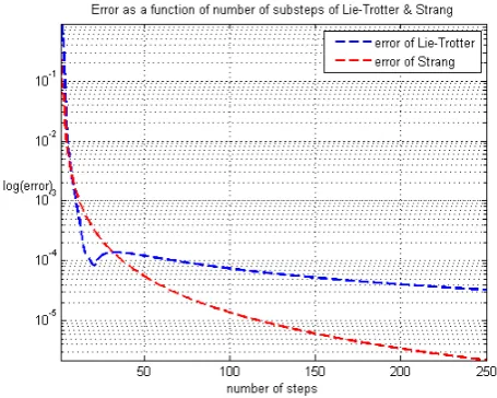
[image:4.595.331.542.259.437.2]

com-parison between Lie-Trotter splitting error and Strang split-ting error againstNFigure 2.

Figure 1. Comparison between Numerical solution of exponential Lie-Trotter splitting and exponential strang splitting for∆t= 0.0126

[image:4.595.316.544.541.723.2]

(5)

7 Conclusions

This Paper discussed the Lie-Trotter and Strang splitting method for ODE system.The Strang method proved that the convergence happened with small data. The numerical solu-tion is calculated up toT = π. We notice that for a small number of mesh points, the Strang splitting method has less errors than the Lie-Trotter splitting method. For large num-ber of mesh points we notice from Figure 2 that the Strang splitting is much better than the Lie-Trotter splitting. More-over Table 1 shows that the Lie-Trotter splitting method is of first order and Strang splitting method is of second order.

REFERENCES

[1] A. B´atkai, and P. Csom´os, and G. Nickel. Operator splittings and spatial approximations for evolution equations. Journal of Evolution Equations, 9(3):613–636, 2009.

[2] F. Castella, P. Chartier, S. Descombes, and G. Vilmart. Split-ting methods with complex times for parabolic equations. BIT Numerical Mathematics, 49(3):487–508, 2009.

[3] A. Chertock, Charles R Doering, E. Kashdan, and A. Kurganov. A fast explicit operator splitting method for passive scalar advection. Journal of Scientific Computing, 45(1-3):200–214, 2010.

[4] S. Descombes and M. Thalhammer. An exact local error representation of exponential operator splitting methods for evolutionary problems and applications to linear schr¨odinger equations in the semiclassical regime. BIT Numerical Mathematics, 50(4):729–749, 2010.

[5] I. Farag´o and A. Havasi. Consistency analysis of operator splitting methods for C0-semigroups expression. In Semi-group Forum, pages 125–139. Springer, 2007.

[6] E. Hansenn and A. Ostermann. High order splitting methods for analytic semigroups exist. BIT Numerical Mathematics, 49(3):527–542, 2009.

[7] S. Blanes, F. Casas, and A. Murua. On the linear stability of splitting methods. Foundations of Computational Mathemat-ics, 8(3):357–393, 2008.

[8] P. Csomós, I. Faragó, and Á. Havasi. Weighted sequential splittings and their analysis. Computers & Mathematics with Applications, 50(7):1017–1031, 2005.

[9] E. Faou, A. Ostermann, and K. Schratz. Analysis of exponen-tial splitting methods for inhomogeneous parabolic equations. IMA Journal of Numerical Analysis, 35(1):161–178, 2015.

[10] E. Hansen and A. Ostermann. Exponential splitting for unbounded operators. Mathematics of computation, 78(267):1485–1496, 2009.

[11] A. Ostermann and K. Schratz. Stability of exponential operator splitting methods for noncontractive semigroups. SIAM Journal on Numerical Analysis, 51(1):191–203, 2013.

[12] Y. Yazici. Operator splitting methods for differential equa-tions. PhD thesis, Izmir Institute of Technology, 2010.

[13] Andrew Y. Ng, Michael I. Jordan, and Yair Weiss. On spectral clustering: Analysis and an algorithm. Advances in neural information processing systems, 2:849–856, 2002.

[14] P. Das and V. Mehrmann, Numerical solution of singularly perturbed convection-diffusion-reaction problems with two small parameters, BIT Numer. Math., 56, 51-76, 2016.

[15] P. Das, Comparison of a Priori and a Posteriori Meshes for Singularly Perturbed Nonlinear Parameterized Problems, J. Comput. Appl. Math., 290, 16-25,2015.

[16] P. Das and V. Mehrmann, Upwind based parameter uniform convergence analysis for two parametric parabolic convection diffusion problems by moving mesh methods, Proc. Appl. Math. Mech., 15, 591-592, 2015.

[17] P. Das and S. Natesan, Adaptive mesh generation for singu-larly perturbed fourth order ordinary differential equations, Int. J. Comput. Math., 92(3), 562-578, 2015.

[18] P. Das and S. Natesan, Richardson extrapolation method for singularly perturbed convection-diffusion problems on adaptively generated mesh, CMES Comput. Model. Eng. Sci 90, 463-485, 2013.