Cellular Automation: A discrete approach for modeling and simulation of Artificial Life Systems

www.ijsrp.org

Cellular Automation: A discrete approach for modeling

and simulation of Artificial Life Systems

Ashwani Kumar

Department of Computer Science & Engineering, F.E.T. Agra College, Agra, (U.P.), INDIA

Abstract- Cellular Automation

“Cellular Automation” (CA) is a decentralized

computing model providing an excellent platform for performing complex computation with the help of only local information. Researchers, scientists and practitioners from different fields have exploited the CA paradigm of local information, decentralized control and universal computation for modeling different applications.

This article provides a survey of available literature of some of the methodologies employed by researchers to utilize cellular automata for modeling purposes. The survey introduces the different types of cellular automation being used for modeling and the analytical methods used to predict its global behaviour from its local configurations. It further gives a detailed sketch of the efforts undertaken to configure the local settings of CA from a given global situation; the problem, which has been traditionally termed as the inverse problem. Finally, it presents the different fields in which CA have been applied. The extensive bibliography provided with the article will be helpful to the new entrant as well as researchers working in this innovative field of computer science.

Cellular Automation are those mathematical models that are used for developing and understanding those systems in which several components acts and interact together to produce rather complicated patterns that reflects / possesses a complex behaviour. Cellular Automata may be viewed as computers, in which data represented by initial configuration is processed by time evolution. Cellular Automata is a model that can be used to show that how the elements of a system interact with each other. Each element of the system is assigned a cell. The cell can be 2D square, 3D blocks, or another such as hexagonal.

A Cellular Automata is an n-dimensional array of simple cells where each cell may be in any one of k-states. At each tick of the clock a cell will change its state based on the states of the cells in a local neighbourhood. Typically, the rule for updating the state does not change over time, and is applied to the whole grid simultaneously. So Cellular Automata is a regular grid of cells, each cell is one of finite number of k possible states. States of the cell is updated synchronously by identical iteration rules. Due to its simplicity the CA rules can be used for modeling and simulating the complex behaviour of living and as well as non-living systems.

Artificial Life Systems

“Artificial Life” (ALife) is a Life made by Human rather than Nature. i.e. The study of man made systems that exhibit characteristics of natural living systems. “ALife is the study of non-organic organisms, beyond the creations of nature, that possess the essential properties of life as we understand it, and whose environment is artificially created in an alternative media, which very often is a programmable machine, i.e. none other than a digital computer.” “ALife is study about the evolution of agents, or populations of computer-simulated life forms in artificial environments.” In particular we describe an attempts concerning three main properties of living beings:

 Reproduction

 Emergent Properties

 Evolution

Modeling & Simulation of ALife Systems can be done very effectively via Cellular Automation, because both of these two paradigms are discrete in nature. CA & ALife are the modern, emergent, and advance technologies of computer science and are used to study the evolution, changes, and survival of various life forms (natural as well as artificial). Almost during the last five decades the various researches have shown that Cellular Automation & Artificial Life, both have their deep roots within Computer Science.

Here our attempt is just to explore the implementation possibilities of Alife Systems via Cellular Automation. The issues, which we will discuss later on in this research paper, are still going on in the field. In this research paper we not only described the “Fundamental concepts of CA”, but also discussed “Its correlation with ALife” in different aspects, which is no doubt the most advanced, sophisticated, and appealing areas of Computer Science. Besides this, the research paper also highlights the flavor of the kind of the work that is being done by various researchers to understand, develop, and implement the ALife Systems via Cellular Automation in synthetic world.

Index Terms- Cellular Automation, Artificial Life Systems,

www.ijsrp.org I. INTRODUCTION & CORELATION OF

CELLULAR AUTOMATA & ALIFE

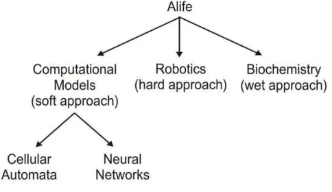
This article guides a stepwise walk. Study into Artificial Life is conducted primarily at three levels, these are:

1. Wetware – Using bits from biology (e.g. RNA, DNA) to investigate evolution.

2. Software – Simulating biological systems.

3. Hardware – For instance, robotics.

Besides this there are two distinct philosophies:

1. Strong ALife – Life is not just restricted to a Carbon-based chemical process. Life can be created in silicon.

2. Weak ALife – Computer simulations are just simulations and investigations of life.

Figure (a): ALife Study

II. HISTORICAL BACKGROUND OF CELLULAR AUTOMATION

The concept of Cellular Automation was originally discovered in the 1940‟s by Stanislaw Ulam and John von Neumann, while they were contemporaries at Los Alamos National Laboratory. While studied some throughout the 1950s and 1960s, it was not until the 1970‟s and Conway's Game of Life, a two dimensional cellular automation, that interest in the subject expanded beyond academia.

In the 1980‟s, Stephen Wolfram engaged in a systematic study of one-dimensional cellular automata, or what he calls elementary cellular automata; his research assistant Matthew Cook showed that one of these rules is Turing-complete. Wolfram published A New Kind of Science in 2002, claiming that cellular automata have applications in many fields of science and

technology. These include computer processors and

cryptography.

The primary classifications of cellular automata as outlined by Wolfram are numbered one to four. They are, in order, automata in which patterns generally stabilize into homogeneity, automata in which patterns evolve into mostly stable or oscillating structures, automata in which patterns evolving in a seemingly chaotic fashion, and automata in which patterns become extremely complex and may last for a long time, with stable local structures. This last Class are thought to be computationally universal, or capable of simulating a Turing machine. Special types of cellular automata are those which are

reversible, in which only a single configuration leads directly to

a subsequent one, and totalistic, in which the future value of individual cells depend on the total value of a group of neighboring cells. Cellular automata can simulate a variety of real-world systems, including biological and chemical ones. There has been speculation that cellular automata may be able to model reality itself.

Cellular automata are often simulated on a finite grid rather than an infinite one. In two dimensions, the universe would be a rectangle instead of an infinite plane. The obvious problem with finite grids is how to handle the cells on the edges. How they are handled will affect the values of all the cells in the grid. One possible method is to allow the values in those cells to remain constant. Another method is to define neighbourhoods differently for these cells. One could say that they have fewer neighbors, but then one would also have to define new rules for the cells located on the edges. These cells are usually handled with a toroidal arrangement: when one goes off the top, one comes in at the corresponding position on the bottom, and when one goes off the left, one comes in on the right. (This essentially simulates an infinite periodic tiling, and in the field of partial differential equations is sometimes referred to as periodic boundary conditions.) This can be visualized as taping the left and right edges of the rectangle to form a tube, then taping the top and bottom edges of the tube to form a torus (doughnut shape). Universes of other dimensions are handled similarly. This is done in order to solve boundary problems with neighbourhoods, but another advantage of this system is that it is easily programmable using modular arithmetic functions. For example, in a 1-dimensional cellular automation like the examples below, the neighbourhood of a cell

x

t is:

Figure (b): A torus, a toroidal shape

www.ijsrp.org John Von Neumann is widely credited with the

origination of the “Stored Program Concept”, that forms the basis of working of a vast majority of machines in today‟s era. But his contribution to the advancement in ALife studies is no less compelling, although relatively unknown.

“Can a machine reproduce itself?” This question was first posed by John Von Neumann in the early 1950‟s and explored by him before his untimely death in 1957. Specifically he asked whether a machine could create a copy of itself, which in turn could create more copies (in analogy to nature).

John Von Neumann wished to investigate necessary logic for the reproduction/self-reproduction. He was not interested, nor he did have the tools, in building a working machine at the bio-chemical or genetic level. Remember that at that time DNA had not yet been discovered as the genetic material in nature.

One such example is John Von Neumann‟s model of “Cellular Automation”, where the basic units are the “Grid Cells” and the observed phenomena involve composite objects consisting of several cells. A machine in the Cellular Automata model is a collection of cells that can be regarded as operating in unison. For example if a square configuration of four black cells exists, that appears at each time step one cell to the right, then we say that square acts as a machine moving right.

John Von Neumann used this simple model to describe a universal constructing machine, which can read assembly instructions of any given machine, and construct that machine accordingly. These instructions are the collection of cells of various colors, as the new machine after being assembled – indeed any compound element on the grid is simply a collection of cells.

John Von Neumann‟s “Universal Constructor” can build any machine when given the appropriate assembly instructions. If these consist of instructions for building a universal constructor, then the machine can create a duplicate of itself; that is, it will reproduce. Should we want the offspring to reproduce as well, we must copy the assembly instructions and attach them to it. In this manner the John Von Neumann showed that a reproductive process is possible in Artificial Machines (ALife Systems). One of the John Von Neumann‟s main conclusions was that the reproductive process uses the assembly instructions in two distinct manners:

1. As interpreted code.

(During actual assembly).

2. As uninterrupted data.

(Copying of assembly instructions to offspring).

During the following decade when the basic genetic mechanisms began to unfold, it became clear that nature had adopted the John Von Neumann‟s conclusions. The process by

which assembly instructions (i.e. DNA) are used to create a working machine (i.e. proteins), indeed makes dual use of information: As interpreted code and as uninterrupted data. The former is referred to in biology as “Translation” and later is referred to as “Transcription” in the terminology of computer science.

This description demonstrates the underlying principle of ALife. The field draws researchers from different streams such as computer science, physics, biology, chemistry, economics philosophy and so on. While biological research is essentially analytic, trying to break down the complex phenomena into their basic components, ALife is synthetic, attempting to construct phenomena from their elemental units. As such ALife complements traditional biological research by exploring new paths in the quest toward understanding the grand and ancient puzzle called “What is Life?”

IV. COMPONENTS OF CELLULAR AUTOMATA

Cellular automata may be considered as information

processing systems, their evolution performing some

computation on the sequence of site values given as the initial state. Cellular Automation has four components:

(1) The Physical Environment: The term physical environment indicates the physical platform on which CA is computed. It normally consists of discrete lattice of cells with rectangular, hexagonal etc shown in Figure (e). All these cells are equal in size. They can be finite or infinite in size and its dimensionality can be 1 (a linear string of cells called an elementary cellular automation or ECA).

(2) The Cell’s States: Every cell can be in a particular state where typically an integer can determine the number of distinct states a cell can be in, e.g. (binary state). Generally, the cell is assigned with an integer value or a null value based upon its state. The states of cells collectively are called as “Global configuration”. This convention clearly indicates that states are local and refer to cells, while a configuration is global and refers to the whole lattice.

(3) The Cell’s Neighbourhoods: The future state of a cell is mainly dependent on its state of its neighbourhood cell, so neighbor-hood cell determines the evolution of the cell. So generally, the lattices vary as one-dimensional and two-dimensional. In one-dimensional lattice, the present cell and the two adjacent cells form its neighbourhoods, whereas in the context of two-dimensional lattice there is four adjacent cells which acts as the neighbourhoods. Therefore, it is clear that as the dimensionality (entropy) increases the number of adjacent cells also increases.

www.ijsrp.org subsequently applied to all the cells in parallel. Typically, the

same rule is used for all the cells (if the converse is true, then the term hybrid CA is used). When there are no stochastic components present in this rule, we call the model a deterministic CA, as opposed to a stochastic (also called probabilistic) CA.

V. MATHEMATICAL MODEL OF CELLULAR AUTOMATION

Formally, a Cellular Automation is represented by the 4-tuple

{ Z, S, N, f } where:

Z: is the finite or infinite lattice.

S: is a finite set of cell states or values.

N: is the finite neighbourhood.

F: is the local transition function defined by

the transition table or the rule.

The lattice is a finite or infinite discrete regular grid of cells on a finite number of dimensions. Each cell is defined by its discrete position (an integer number for each dimension) and by its discrete value (one of a finite set of integers). Time is also discrete. The future state of a cell (time t+1) is a function of the present state (time t-1) of a finite number of cells surrounding the observed cell called the neighbourhood.

VI. EMERGENT BEHAVIOUR OF CELLULAR AUTOMATION

“Global behaviour or pattern arises from the local interactions.”

A fundamental precept of CA is that the local transition function determining the state of each individual cell at a particular time step should be based upon the state of those cells in its immediate neighbourhood at the previous time step or previous time steps.

Thus the rules are strictly local in nature and each cell becomes an information-processing unit integrating the states of the cells around it and altering its own state unison with all the others at the next time step in accordance with the stipulated rule.

Thus many global patterns of the system are an „emergent' feature‟ of the effect of the locally defined transition function. that is, complex global featurescan emerge from the strictly local interaction of individual cells each of which is only aware of its immediate environment.

VII. CELLULAR AUTOMATION AS A TRANSITION FUNCTION

Number of neighbors of a cell including that cell also = 2r + 1, Where r = 1, 2, 3,……

Basically r is the dimension of C.A. Besides this the number of allowable states also play an important role in Cellular Automata. Here it is denoted by k. For the simplest case k=2 (binary states). The states of the cell are represented by:

0 : Dead State 1 : Live State

Usually we keep fix the value of k= 2, for all cases.

If r=1, It results 1D-CA. If r=2, It results 2D-CA.

VII. CELLULAR AUTOMATA MODEL: FUNDAMENTAL FEATURES, AND SPECIFICATIONS

CA: The Fundamental Features

The three most fundamental features of Cellular Automation are:

(1) Uniformity: All cell states updated by same set of rules.

(2) Synchronity: All cell states updated simultaneously.

(3) Locality: The rules are local in nature.

CA: The Specification

(1) A neighbourhood function that specifies which of the adjacent cell affects its state.

(2) A transition function that specifies mappings from state

of neighbor cells to state of given cell.

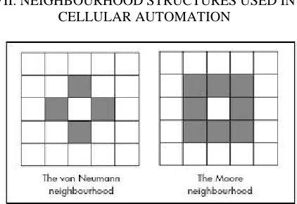
VII. NEIGHBOURHOOD STRUCTURES USED IN CELLULAR AUTOMATION

Figure (c): Examples of neighbourhood structures

www.ijsrp.org Moore neighborhood are termed “nine-neighbor square”.

Totalistic cellular automation rules take the value of the center site to depend only on the sum of the values of the sites in the neighbourhood. With outer totalistic rules, sites are updated according to their previous values, and the sum of the values of the other sites in the neighbourhood. Triangular and hexagonal lattices are also possible, but are not used in the examples given here. Notice that five-neighbor square, triangular, and hexagonal cellular automation rules may all be considered as special cases of general nine-neighbor square rules.

VIII. ONE-DIMENSIONAL CELLULAR AUTOMATION (SOME EXAMPLES)

Rule Number: 30

Current

Pattern _{111 110 101 100 011 010 001 000}

New State for Center

Cell

0 0 0 1 1 1 1 0

Figure (d): Rule - 30

Figure (e): Conus textile exhibits a cellular automation pattern (Rule-30) on its shell.

For example the widespread species ConusTextile bears a pattern resembling Wolfram's Rule-30 cellular automation.

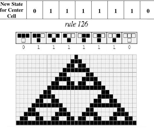
Rule Number: 126

Current

Pattern _{111 110 101 100 011 010 001 000}

New State for Center

Cell 0 1 1 1 1 1 1 0

Figure (f): Rule - 126

IX. CELLULAR AUTOMATION RULES: AT A GLANCE

Table (a): Cellular Automata Rules

X. THE CLASSIFICATION WITHIN ONE DIMENSIONAL CELLULAR AUTOMATA MODEL

Empirical studies strongly suggest that the qualitative properties of one-dimensional cellular automata are largely independent of such features of their construction as the number

CELLULAR AUTOMATION WITH BINARY STATES

NEIGHBORS (N)

(1+N) NO. OF

PATTERNS

NO. OF RULES

1-D

TWO ( L, R )

1+2=3 23= 8 (3 Bit Pattern)

28= 256 Rules

2-D

FOUR ( L, R, U, D )

1+4=5 25_{= 32}

(5 Bit Pattern)

232

Rules

2-D

EIGHT

( Boundary Cells )

1+8=9 29= 512 (9 Bit Pattern)

2512 Rules

3-D

TWENTY SIX ( Cells lies on all six surfaces )

1+26=27 227

www.ijsrp.org of possible values for each site, and the size of the

neighbourhood.

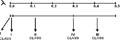
In order of complexity the four qualitative classes of behaviour have been identified by Wolform in one-dimensional cellular automata. While earlier studies in cellular automata tended to try to identify type of patterns for specific rules, Wolfram's Classification was the first attempt to classify the rules themselves. Starting from typical initial configurations, these are:

 Class-l Cellular Automata- It evolves to homogeneous final states. Class-l cellular automata evolve from almost all initial states to a unique final state, analogous to a fixed point. Nearly all initial patterns evolve quickly into a stable, homogeneous state. Any randomness in the initial pattern disappears.

 Class-2 Cellular Automata- It yields separated periodic structures. Class-2 cellular automata evolve to collections of periodic structures, analogous to limit cycles. The contraction of the set of configurations generated by a cellular automation is reflected in a decrease in its entropy or dimension. Starting from all possible initial configurations (corresponding to a set defined to have dimension one). Nearly all initial patterns evolve quickly into stable or oscillating structures. Some of the randomness in the initial pattern may filter out, but some remains. Local changes to the initial pattern tend to remain local. So for Class-2 type the stable or oscillating structures may be the eventual outcome, but the number of steps required to reach this state may be very large, even when the initial pattern is relatively simple. Local changes to the initial pattern may spread indefinitely. Wolfram's Class-2 can be partitioned into two subgroups:

(1) Stable (fixed) Rules

(2) Oscillating (periodic) Rules

 Class-3 Cellular Automata- It exhibits chaotic behaviour, and yield aperiodic patterns. Small changes in initial states usually lead to linearly increasing regions of change. Class-3 cellular automata yield sets of configurations with smaller, but positive, dimensions. These sets are directly analogous to the chaotic (or "strange") attractors found in some continuous dynamical systems. Nearly all initial patterns evolve in a pseudo-random or chaotic manner. Any stable structures that appear are quickly destroyed by the surrounding noise. Local changes to the initial pattern tend to spread indefinitely.

 Class-4 Cellular Automata- It exhibits complicated localized and propagating structures. It is conjectured that Class-4 cellular automata are generically capable of universal computation, so that they can implement arbitrary information-processing procedures. Nearly all initial patterns evolve into structures that interact in complex and

interesting ways, with the formation of local structures that are able to survive for long periods of time. Wolfram has conjectured that many, if not all Class-4 cellular automata are capable of universal computation. This has been proven for Rule-110 and Conway's Game of Life.

Wolfram, in A New Kind of Science and several papers dating from the mid-1980s, defined four classes into which cellular automata and several other simple computational models can be divided depending on their behaviour.

Figure (g): Wolform‟s Classes for Elementary Cellular Automation

Wolfram's Classification has been empirically matched to a clustering of the compressed lengths of the outputs of cellular automata. There have been several attempts to classify cellular automata in formally rigorous classes, inspired by the Wolfram's Classification. For instance, Culik and Yu proposed three well-defined classes (and a fourth one for the automata not matching any of these), which are sometimes called Culik-Yu Classes; membership in these proved to be undecidable.

These definitions are qualitative in nature and there is some room for interpretation. According to Wolfram, "…with almost any general classification scheme there are inevitably cases which get assigned to one class by one definition and another class by another definition. And so it is with cellular automata: there are occasionally rules...that show some features of one class and some of another."

Dynamical systems theory methods may be used to investigate the global properties of cellular automation. One considers the set of configurations generated after some time from any possible initial configuration. Most cellular automation mappings are irreversible (and not surjective), so that the set of configurations generated contracts with time.

XI. 1-D Vs 2-D CELLULAR AUTOMATA

Entropy or dimension gives only a coarse

www.ijsrp.org of a one-dimensional cellular automation can be shown to form a

regular language: the possible configurations thus correspond to possible paths through a finite graph. For most Class-3 and Class-4 cellular automata, the complexity of this graph grows rapidly with time, so that the limit set is presumably not a regular language. This paper reports evidence that certain global properties of two- dimensional cellular automata are very similar to those of one-dimensional cellular automata.

Many of the local phenomena found in two-dimensional cellular automata also have analogs in one dimension. However, there are a variety of phenomena that depend on the geometry of the two-dimensional lattice. Many of these phenomena involve complicated boundaries and interfaces, which have no direct analog in one dimension.

1D 2D-Square 2D-Hexagonal

Figure (h): Various arrangements of neighbor cells in 1-D and 2-D spaces

Many definitions are carried through directly from one dimension, but some results are rather different. In particular, the sets of configurations that can be generated after a finite number of time steps of cellular automation evolution are no longer described by regular languages, and may in fact be no recursive. As a consequence, several global properties that are decidable for one-dimensional cellular automata become undecidable in two dimensions.

XII. COMPLEXITY OF ALIFE SYSTEMS

“Life is a complex system: It is a dynamic system that can keep on changing and evolving over a great period of time without dying.”

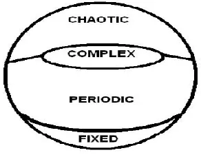
If the amount of information exchange in a system is varied from low to high, it gives “Fixed”, “Periodic”, and “Chaotic” systems in that order. Somewhere in between, a system exhibits “Complex” behaviour. Accordingly, each unit (cell) in a system dies, freezes, pulsates, or behaves in a very complex manner.

CHANGE EVOLUTION DEATH

FIXED NO NO NO

PERIODIC YES NO NO

CHAOTIC YES YES YES

COMPLEX YES YES NO

Table (b): Complexity of ALife Systems

Figure (i): Various models of Life

XIII. FUNDAMENTAL APPROACHES USED TO IMPLEMENT ARTIFICIAL LIFE SYSTEMS

 NEURAL NETWORKS

 EVOLUTIONARY ALGORITHMS

1. Genetic Programming

2. Evolutionary Programming

3. Classifier Systems

4. Lindenmeyer Systems

 CELLULAR AUTOMATA

XIV. TWENTY PROBLEMS IN CELLULAR AUTOMATION

1. What overall classification of CA can be given?

2. What are the exact relations between entropies and Lyapunov exponents for CA?

3. What is the analogue of geometry for the configuration space of a CA?

4. What statistical quantities characterize CA behaviour? 5. What invariants are there in CA evolution?

6. How does thermodynamics apply to CA? (broken time symmetry problem)

7. How is different behaviour distributed in the space of CA rules?

8. What are the scaling properties of CA?

9. What is the correspondence between CA and continuous

systems?

10. What is the correspondence between CA and stochastic

systems?

11. How are CA affected by noise and other perturbations?

12. Is regular language complexity generically

non-decreasing with time in 1-D CA? 13. What limit sets can CA produce?

14. What are the connections between the computational and statistical characteristics of CA?

15. How random are the sequences generated by CA?

16. How common are computational universality and

undesirability in CA?

www.ijsrp.org

18. How common is computational irreducibility in CA?

19. How common are computationally intractable problems

about CA?

20. What higher-level descriptions of information

processing in CA can be given?

XV. CONCLUSION

Cellular Automation & ALife thus are advanced innovative and interesting field of computer science. The above detailed description of activities is sufficient to show that the activities pursued under this label are aimed at replicating some of the very basic activities of living beings. The basic issues of Artificial Life and Artificial Intelligence pertain to the issues investigated. Whereas AI has traditionally concentrated on the complex functions of human beings, such as chess playing, text comprehension, medical diagnosis, and so on. ALife mainly

concentrates on basic natural behaviours, emphasizing

survivality in complex environments. According to Brook‟s, an examination of the evolution of life on earth reveals the most of the time was spent developing the basic intelligence. The elemental faculties evolved to enable mobility in a dynamic environment and sensing of the surroundings to a degree sufficient to achieve the necessary maintenance of life and reproduction.

The issues dealt with by AI appeared only very recently on the evolutionary scene and mostly in humans. This suggests that the problem-solving behaviour, language, expert knowledge, and reason are all rather simple once the essence of being and reacting is available. This idea is expressed in the title of one of the Brook‟s papers, „Elephants Don‟t Play Chess‟, suggesting that these animals are no more highly intelligent and able to survive and reproduce in a complex dynamic environment.

Celluar Automation is thus a powerful approach for studying the behaviour of Alife Systems by simply assuming the real environment, its objects, and activities (which are of course continuous in nature) as suppose to existing and happening in discrete manner. Most of the species and their behaviour have been simulated successfully via Cellular Automation. Alife Systems are basically complex in nature and their behaviour totally depends on the creativity and interest of the developer. Alife Systems are just “Machines with Life”.

On the other hand in context to the Cellular Automation, every cell is treated as a logical machine. As far as if we talk about the scope of developing such type of machines that possesses life, we must believe that these machines can do a lot of tasks of different domains with significant accuracy and effeciency. Artificial Life based Systems can even does those tasks that are hard and almost impossible for most of us. So from the implementation point of view, Cellular Automation is a milestone in the field of Artificial Life. But this is not the limit, because a lot of researches on real and artificial world have shown that human beings and nature also obeys the “Principles of the Cellular Automation”. The only thing that is being left is

that, upto how much extent we are able to explore the unexplored world via Cellular Automation.

REFERENCES

[1] Two-Dimensional Cellular Automata, Norman H. Packard l and Stephen Wolfram, 1985 Plenum Publishing Corporal ion

[2] Robert A. Wallace, Biology – The Science of Life, Harper Collins, 1996, The Fourth Ed.

[3] Joel L. Schiff, “Cellular Automata”: A discrete view of the world

[4] John H. Holland, Induction: Processes of Inference, Learning, and Discovery, The MIT Press, 1989

[5] John R. Koza, Genetic Programming II, The MIT Press, 1994

[6] John H. Holland, Adaptation In Natural & Artificial Systems, The MIT Press, 1992

[7] Ashwani Kumar, “An Overview of Abstract & Physicial Characteristics of Artificial Life Systems.”, International Journals of Scientific Research Publication, Dec. 2012

[8] H. Mohan and C. Patwardhan, “Alife Systems: An Overview”, Proceedings of the National Seminar- SASESC-2000, Allied Publishers Ltd. 2000

[9] http://www.cse.psu.edu/~datta/Present/alife.ppt [10] http://www.en.wikipedia.org/wiki/Cellular_automation [11] http://www.findthatpowerpoint.com

AUTHOR (S):

First Author: Ashwani Kumar ( M.E. / CS&E ) Assistant Professor, Department of Comp. Sc. & Engg. F.E.T. Agra College, Agra, (U.P.), India

Email: [email protected]