Different Methods for Partitioning the Phase Space of a
Dynamic System
Abir Hadriche, Nawel Jmail
Laboratory of Electronics and Information Technologies Sfax University, Sfax, Tunisia.
Ridha Elleuch
Laboratory of G´eoressouces, Mat´eriaux, Environnement. Physics Department
Faculty of Sciences of Sfax Sfax University, Sfax, Tunisia.
Laurent Pezard
Institut de Neurosciences des Syst`emes (UMR S 1106) Aix-Marseille University, INSERM, Marseille, France.
ABSTRACT
In symbolic dynamics, the definition of a symbolic sequence from a continuous times series depends on the use of an appropriate par-tition of the phase space. In fact, the best way is to estimate a gen-erating partition.
However, it is not possible to find generating partitions for most ex-perimental observations because such partitions do not exist when noise is present.
In this paper, different partition methods applied to stochastic and chaotic system will be compared in order to choose one which con-serves system entropy rate. This partition is called a Markov parti-tion.
General Terms:
Markov partition, symbolic dynamic
Keywords:
Markov partition, generating partition, symbolic sequence, entropy rate
1. INTRODUCTION
Symbolic dynamics approach allows to study a discrete dynamical system equivalent to the continuous dynamics of a physical system. This approach was pioneered by Hadamard in 1898 [12] who sug-gested the idea to split the state space into a finite number of parts, each part having a name (usually a number or letter of alphabet). All the points of the phase space are given the name of the part to which they belong.
Given a partition of the state space, associating to each pointxan infinite word describing its trajectory is a transformation from a complex application to a simple one. But the state space becomes more complex, it is now a set of infinite words which allows to un-derstand the structure of the dynamics.
The main issue of symbolic dynamics is to seek for a partition of the state space that describes the trajectories of points and verify
the constraint to represent the dynamics in a simple way. This sym-bolic method allows to overcome the limitations of analytical ap-proaches, while retaining some key properties in terms of the dy-namics.
This type of partition is called a Markov partition because of its connection to discrete time Markov processes.
In the dynamical systems literature, one typically search for a gen-erating partition which has strong theoretical settings. Neverthe-less, a generating partition is hardly determined on the basis of ex-perimental data [5].
Note further that every Markov partition is generating, but the con-verse is not necessarily true [5].
In this paper, different methods for partitioning the phase space of a dynamic system will be presented such as methods of vector quantification (self organizing maps [16] and K-means algorithm [20]) and methods of numerical approximation of dynamical systems (varcluster [1] and subdivision [7]).
These methods will be tested in chaotic and stochastic dynamic systems to extract the best partition associated to Markov process. This paper is organized as follows: the first section describes various phase space partition methods, these methods will be used in the following section to quantify discrete stochastic and chaotic systems in order to estimate their performance and select the best one.
2. METHODS
2.1 Different partition methods
In this paper, the phase space of each dynamical system is denoted E.
In this space, a simulation ofTsseconds leads to a sequence of row vectors~e(t) = (e1(t), . . . , eN(t))witht= 0, . . . , T−1withT =
Ts/∆tthe number of samples simulated by∆tintegration step. The partition ofEcorresponds to the definition of non-overlapping regionsmi so that
S
imi = E and
T
2.1.1 First method: K-means. This method of clustering was in-troduced by MacQueen [20] and its algorithm is developed by Har-tigan and Wong 1979 [14]. This method is the simplest one that can solve the problems of partitioning. Its seeks the easiest way to classify the data in some m numbers region in state space [6], [21]. The idea is to represent each group by its mean centroid calledc. The steps of this algorithm are:
—Choose randomlymgroups.
—Regroup centroids that are close enough. —Recalculate the positions of themnew centroids.
—Repeat last two steps until the minimization of measurement er-ror given by the sum of square erer-rors calculated between each point and each group centroid.
E=
m
X
j=1
X
i
kxji−cjk2
(1)
With kxji −cjk2 is the distance measured betweenxj i points included injthgroup withc
jcentroid.
2.1.2 Second method: Self organizing maps. Unlike the k-means method, the self-organizing maps (SOM) [16] allows a rapid un-supervised learning of individuals (the states of systems in phase space).
It relies on a neural network distributed uniformly in a space of2
or3dimensions. Each neuron is defined by a vector in the space of individuals, called weight vector. Individuals are presented succes-sively to the network.
For each individualxk withk ∈ {1, ..., T}, the nearest neuron (calledBest Matching Unit, BMU) and its vicinity in the network are modified so that together they are close to the individual. This algorithm takes place mainly in three phases:
—Initialization the weights of output neurons (small random val-ues).
—Presentation of an example of the base and determining the out-put neuron closest to the example (BMU).
Finally, we determine the Euclidean distance between the exam-ple and all the output neurons characterized by their weight. The neuroniis selected:
kwi−xkk ≤ kwj−xkk ∀j6=i (2)
Euclidean distance is used to calculate the activation of each out-put neuron as follows:
αj=
A B+Ckwj−xkk
(3)
Withxkis the input of the map,wiis the weight of the neuron andA,B, andCare any constants.
—Weights are adapted using:
wj(t+ 1) =wj(t) +α(t)v(j, i, t)(x−wj(t)) (4)
α(t) is learning rate andv(j, i, t)is neighbors function. Only the weights of neurons in the vicinity of the selected one are changed. Learning rateα(t) is a function that decreases over time:
α(t) = α0 1 +Kαt
(5)
The neighbors function v(j, i, t) is a Gaussian function that evolves such as :
v(j, i, t) = exp
−d
2(j, i)
2σ2(t)
(6)
This is repeated untilreaches a threshold.is defined as:
=
Pn
i=1kwki−xik
2
n (7)
for n iterations.
2.1.3 Third method: Subdivision. This partitioning method is in-troduced by Hohmann and Dellnitz [7] inspired by Ulam-Galerkin discretization process [22]. It was used for the quantification of ran-dom dynamical systems (stochastic oscillations of Van Der Pol) [15], and also of chaotic systems (logistic and H´enon applications) [8].
We start with a dynamic system given by the application f : R→RN, the algorithm considers the partition in the first place a rectangleQgiven by:
Q=R(c, r) :={x= (xi)∈RN:|xi−ci| ≤rifori= 1, . . . , N} (8) Withc= (ci),r=ri∈Rdand a space phase of the system given by:
AQ:=
\
n≥0
fn(Q) (9)
and ignoring any dynamic outside the rectangleQ.
The selection of regions is valid in the rejection of all empty rect-anglesQthat doesn’t contain an image off(xiin phase space).
2.1.4 Fourth method: Varcluster. This approach of partition of the state space is proposed by Allefeld et al. [1].
They defined the state space byNvariables1(x
1, x2, . . . , xN) =
x to be discretized, resulting in a set of compound microstates which forms the basis for further analysis.
This algorithm uses a recursive bi-partitioning approach: for a given set ofT data pointsM = {x(t)},t = 1. . . T, the direc-tion of maximal variance is determined, i.e a unit vectore,|e|= 1, such thatvarm(x(t).e) obtains its maximum value. Using the me-dianM ed of the data points’ positions along this direction as a threshold value, the set is divided into two subsets:
M1={x(t)|x(t).e≤M ed} (10)
M2={x(t)|x(t).e > M ed} (11)
The procedure is repeated for each of the resulting subsets. The number of repetition is the numberkof iteration to obtain a se-quence of2ksymbols.
2.1.5 Comparaison between different partition methods. To ex-tract the best partition methods to describe the dynamic system in phase space, we used this strategy:
—Divide the phase space intom = 2k regions using one of the partition methods explained above.
—Calculate transition matrix of the Markov chain:
The dynamics of Markov chain of order1is fully determined by the transition matrixτand stationary distributionπ. Then form
space regions, a matrix of[mxm]dimensions was established (similar to a transfer matrix in statistical physics), whose
tion elements are in general either real or complex weights.
τi,j=
(
τi∈R or C if the transitionmj→miis permitted,
0 else.
(12) Here, letM(k)be an homogeneous Markov chain for partition
k, its transition matrixτ(k) = τ(k)
ij withi, j ∈ {1. . .2 k}; so
the transition probability between states isτ(k) = (τ(k)
i,j) =
(Pr(m(k)(t) =j|m(k)(t−1) =i).
—Normalize this transition matrix:
This step is introduced by Gaveau and Shulman [9], [10], [11]. Letτ(k)be a stochastic matrix with2kdimensions obtained af-ter thekthiteration. To assume thatτ(k)is irreducible matrix so
[10] it has only one eigenvalue of unit norm to be calledλ0, and
order the other eigenvalues by decreasing modulus.
λ0is associated with a strictly positive eigenvector; the
remain-ing2k−1eigenvectors satisfyλ
0 ≡ 1>|λ1| ≥ |λ2|. . .,
cor-respond to right and left eigenvectors that are, respectively,vm andlm, with(m∈2k)regions, so:
τ(k)v
m=λmvm lmτ(k)=λmlm
lm was normalized by hlm|vbi = δmb, and v0 is naturally
normalized byP
iv0(i) = 1.
—Select an alphabet size of symbolic sequence
The choice of the alphabet size plays a crucial role in symbolic time series analysis.
For example, a small value ofkiteration may prove inadequate for capturing the characteristics of the system dynamic. On the other hand, a large value may lead to redundancy and waste of computational resources. The selection of optimal is an area of active research.
An entropy rate approach has been adopted for selecting the al-phabet size [23].
Leth(M(k))denote the entropy rate of the transition matrix for
iterationk[4].
h(M(k)) =−X
i,j
πi(k)τi,j(k)logτi,j(k) (13)
where theπ(k)andτ(k)are both maximum likelihood estimate
of, respectively, the stationary distribution and probability of transition andlogis taken as natural logarithm.
The value of entropy rateh(M(k))increases of iteration withk.
We choosek∗∈ {1, kmax}whereh(M(k))is maximal
(practi-callykmax≈10).
To further incrementk > k∗value, leads to the problem of finite size of symbolic sequence and then the value of entropy rate de-creases. This decrease is due to the finite sizeTof the symbolic sequence.
This effect was shown in our previous work [13] by partionning several time series of Lorenz system with different sizeT using subdivision method.
Also this effect is shown analytically in calculating the entropy rate of a given symbolic sequenceM(k)of sizeT obtained by
using the subdivision partition and the assumption of uniform
transition probabilities. Shannon’s entropyH(M(k))is written
as:
H(M(k)) =− X m∈M(k)
τ(k)(m) logτ(k)(m)
=−2kT
2klog
T 2k
=−Tlog
T 2k
=−T(logT−klog 2)
(14)
And the entropy rate ofM(k)is:
h(M(k)) = lim
k→∞
H(M(k))
k
= lim
k→∞
T
k(klog 2−logT)
= lim
k→∞
Tlog 2− TlogT
k
(15)
In addition, for a sequence of finite sizeTobtained by the parti-tion of subdivision, there will be a maximum ofkiterations such asT = 2kandk→(logT
log 2)and no∞, so (15) equation can be
written as:
h(M(k)) = lim
k→(loglog 2T)
Tlog 2−TlogT
k
= 0 (16)
And the rate of entropy converges to zero fork >> k∗ .
Now, different partitions process will be tested with various dynam-ical system in order to extract the best Markov partition.
3. RESULTS
Numerical simulations were used to check the validity of the ap-proach on systems with known properties. Multivariate indepen-dent and iindepen-dentically distributed Gaussian process and deterministic chaotic system were used to compare these different partition meth-ods.
3.1 White noise
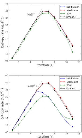
In this section two samples of white noise will be used, the first is a Gaussian noise following a normal distribution with given mean and variance and the second is a uniform noise. Two random systems of5dimensions withT = 30000points were generated. Presume that the white noise is a realization of a random process in which the power spectral density is the same for all frequencies, we can deduce that the theoretical value of the entropy rate is equal tolog(2k)with2kis the number of symbols of the sequence obtained after each iterationk.
Fig. 1. Entropy rate of the meso-scale Markov process (h(M(k))) of
white noise at each iteration (k) calculated in different partitions method. Top: Noise uniform. Bottom: Gaussian noise.
In the next section, these discretization methods will be applied on the phase space of a chaotic system (Lorenz attractor).
3.2 Lorenz chaotic system
The Lorenz system is a three dimensional dynamic system (topol-ogy and metric values are well studied in [19], [17], [18], [2] et [3]) defined by three nonlinear differential equations:
.
x=σ(y−x)
.
y=Rx−y−xz
.
z=−bz+xy
(17)
It is based on three control parameters: the number of Pradtlσ, a ratioRand a parameterbdimensional rolls. (For more details see [17]).
The asymptotic motion in the phase space of this system is related to a chaotic attractor representing an axial symmetry, which is adjusted by control parameters such asσ = 10, R = 28 and
b= 8/3.
Figure 2 depicts16regions of Lorenz attractor obtained after four steps of the subdivision procedure.
Figure 3 includes the values of the entropy rate calculated after a refinement of the partition of phase space.
[image:4.595.360.537.80.218.2]This figure shows the importance of this refinement that correctly describe the dynamics following a convergence of the theoretical value of the entropy rate (≈0.92for the Lorenz attractor computed
[image:4.595.340.520.281.419.2]Fig. 2. Lorenz attractor after four steps of the subdivision procedure. Each color corresponds to one of the 16 meso-states of the system defined by Ulam subdivision procedure.
Fig. 3. Entropy rate of the meso-scale Markov process (h(M(k))) of
Lorenz attractor at each iteration (k) calculated in different partitions method.
with a natural logarithm).
By subdivision process, it was able to reach this theoretical value afterk∗= 7
iterations and to obtain a discrete Markov process with
128states.
As for the case of multivariate random process, an observation of the finite-size effects appears fork > k∗.
4. DISCUSSION
Discretization of phase space of a dynamic system requires choos-ing the correct partition that preserves the dynamic properties of the system.
In this work, four partitions methods were compared among the most used such as: k-means, SOM, varcluster and subdivision. This work is a continuation or even a step to verify a discretization in our previous paper [13] made to transform the microscopic space of measuring brain activity in a mesoscopic space.
Indeed, during this task we compared only two different methods of partition such as subdivision and varcluster and we concluded that the subdivision allowed to obtain satisfactory results to parti-tioning chaotic and stochastic systems.
meth-ods of vector quantification such as k-means and SOM. These four methods were applied to partition the same systems. We concluded that the subdivision method indeed gives the best results.
In fact, this comparison was based on the estimation of the entropy rate of transition matrix of Markov chains. Adding another param-eter of comparison is one of the perspectives of this work. It should also be noted that the application to other dynamic sys-tems of these partition methods is needed to further verify that the subdivision process is among the best ways to discretize the phase space of dynamical systems.
5. REFERENCES
[1] C. Allefeld, H. Atmanspacher, and J. Wackermann. Mental states as macrostates emerging from brain electrical dynam-ics.Chaos, 19:015102, 2009.
[2] Erick.M Bollt. Review of chaos communication by feed-back control of symbolic dynamics.Bifurcation and Chaos, 13:269–285, 2003.
[3] J.P. Bouchaud and P. Doussal. Numerical study of a d-dimensional periodic Lorentz gas with universal properties. Statistical Physics, 41:225–248, 1985.
[4] G. Ciuperca and V. Girardin. On the estimation of the entropy rate of finite Markov chains.Proceedings of the International Symposium on Applied Stochastic Models and Data Analysis, 2005.
[5] J. P. Crutchfield and N. H. Packard. Symbolic dynamics of noisy chaos.Physica D, 7:201–223, 1983.
[6] Pelleg Dan and Moore Andrew. Accelerating exact K-means algorithms with geometric reasoning. In Surajit Chaudhuri and David Madigan, editors,Proceedings of the Fifth Inter-national Conference on Knowledge Discovery in Databases, pages 277–281. AAAI Press, aug 1999.
[7] M. Dellnitz and A. Hohmann. A subdivision algorithm for the computation of unstable manifolds and global attractors. Numerische Mathematik, 75:293–317, 1997.
[8] Michael Dellnitz and Oliver Junge. Set oriented numerical methods for dynamical systems, volume 2. Elsevier, 2002. [9] B. Gaveau and L.S. Shulman. Theory of nonequilibrium
first-order phase transitions for stochastic dynamics.Mathematical Physics, 39:1517–1533, 1997.
[10] B. Gaveau and L.S. Shulman. Dynamical distance: coarse grains, pattern recognition, and network analysis. Sciences Mathematiques, 129:631–642, 2005.
[11] B. Gaveau, L.S. Shulman, and L.J. Shulman. Imaging geome-try through dynamics: the observable representation.Physics A, 39:10307–10321, 2006.
[12] J Hadamard. Les surfaces `a courbures oppos´ees et leurs lignes g´eod´esiques.Biological Cybernetics, 43:59–69, 1898. [13] A. Hadriche, L. Pezard, J.P. Nandrino, H. Ghariani, A.
Ka-chouri, and K.V. Jirsa. Mapping the dynamic repertoire of the resting brain.NeuroImage Journal, 78:448–62, Septem-ber 2013.
[14] J. A. Hartigan and M. A. Wong. A k-means clustering algo-rithm.Applied Statistics, 28:100–108, 1979.
[15] H. Keller and G. Ochs.Numerical approximation of random attractors. Springer, 1999.
[16] T. Kohonen. Self-organized formation of topologically cor-rect feature maps.Proceedings of 5-th Berkeley Symposium on Mathematical Statistics and Probability, 1:281–297, 1982.
[17] Christophe Letellier. Caract´erisation topologique et recon-struction d’attracteurs ´etranges. PhD thesis, Universit´e de Paris, 1994.
[18] Christophe Letellier.syst`emes dynamiques complexes: de la caract´erisation topologique `a la mod´elisation. PhD thesis, 1998.
[19] E.N. Lorenz. Deterministic nonperiodic flow. The Atmo-spheric Sciences, 20:130–142, 1963.
[20] J.B MacQueen. Some methods for classification and analy-sis of multivariate observations. Proceedings of 5-th Berke-ley Symposium on Mathematical Statistics and Probability, 1:281–297, 1967.
[21] Mohd Shukor, Zamzarina, Md. Sap, and Mohd. Noor. Clus-tering technique in data mining: general and research perspec-tive.Teknologi Maklumat, 14:50–63, 2002.
[22] S. Ulam.A collection of mathematical problems.Interscience Publishers, New York, 1960.