Study and Overview on System Feedback Representations in Control Modeling with Artificial Neural Networks (ANN) Platform

Study and Overview on System Feedback

Representations in Control Modeling with

Artificial Neural Networks (ANN) Platform

ABSTRACT

Artificial Neural Network has become one of the most beneficial methods for efficiency improvement of control system engineering and its different aspects. A review study on block diagram representation with effective and satisfactory performance analysis via artificial neural network techniques is proposed in this paper. The implementation of any block diagram with artificial neural networks using MATLAB (R2008b) simulator and the neural modelof the training state and the performance obtained from the graphs is the basic outcome of this paper. A brief literature review on control theory approach with feedback block modeling and signal flow graphs along with the contribution of artificial neural networks in the field of control system is also studied in this paper.

KEYWORDS

Feedback Control Block, Signal Flow graphs(SFG), Artificial Neural Network (ANN), ANNMATLAB (R2008b) Codingand Elman network.

1.

INTRODUCTION

The field control systems is comparatively unique which has become more significant with the progression of technology as it involves an interconnection of the physical components toaccommodate a desired function, involving some kind of controlling activity in it. In control system block diagram is a pictorial embodiment of various practical systems in a very simple way, explaining the cause and effect associationsexisting between input and output of the system[1]. On the other hand, the goal of artificial intelligence is the development of standard models or appropriate algorithms that require machines to perform experimental tasks, at which humans are currently exceeding [2]. A neural network is a massively parallel delivered processor made up of simple processing units(neurons), which has a characteristic ability for storing experimental knowledge and making it available for use matching a normal human brain[3]. This paper deals with a study of the basic block diagram implemented by artificial neural network using MATLAB(R2008b) coding.The block diagram provides a functional explanation of the various elements that comprises of the model of an artificial neuron. The representation of the model is simplified by using

the concept of signal-flow graphs without dropping any of the functional details of the model. Signal-flow graphs with a distinct set of formulas are originally developed by Mason for linear networks. Signal-flow graphs do arrange a neat method for the sketch of the flow of signals in a neural network, which is discussed in this paper [4]. The aim of the paper is to help the researchers in implementing any block diagram representations (which can also be derived from transfer functions) using artificial neural networks in any field of research.

2.

CONTROL THEORY APPORACH

WITH BLOCK MODELLING AND SFG’S

Feedback control system generally involves many steps to design it in the proper way.

The typical outline towards control approach is as follows:

1. The system to be controlled is studied and types of sensors and actuators required to be used andwhere the componentsto be placed are determined.

2. The produced system to be controlled is then modeled.

3. Simplification of the model is done if necessary so that it is tractable.

4. The resulting model is analyzed in order to determine its features.

5. Performance specifications are then determined.

6. The type of controller is chosen to be used.

7. A controller is so designed so thatit meets the requirements, if possible; if not, the guidelines are modified or generalized according to the type of controller sought.

8. The resulting controlled system is then simulated, either on a computer or in a pilot plant.

9. Step 1 is repeated if necessary.

10. Hardware and software are then selected and implemented in the controller.

11. The controller is tuned on-line if necessary.

In consideration to model for a system four objectives are essential.

1. Real physical system: the oneis “out there.”

2. Ideal physical model: obtained by schematically decomposing the real physical system intoideal building

Sayanti Roy

B.tech Student, ECE Dept.

Greater Kolkata College of

Engg&Mgmt, 24 Pgs(S)

W.B., India

Zinkar Das

M.Tech Scholar, EIE Dept.

JIS College of Engineering

Kalyani, Nadia,

W.B., India

SubhamGhosh

Faculty, ECE Dept.

JIS College of Engineering

Kalyani, Nadia,

W.B., India

BiswarupNeogi,

PhD

Faculty, ECE Dept.

JIS College of Engineering

blocks which comprises the resistors, masses, beams, kilns, isotropic media, Newtonianfluids, electrons, and many more.

3. Ideal mathematical model: obtained by applying natural laws to the ideal physical model is mainly composed of nonlinear partial deferential equations, and many more.

4. Reduced mathematical model: derived from the ideal mathematical model by linearization, lumping, and many more; usually based on a rational transfer functions [5].

Control systems have a number of control components which can be represented in a block diagram form. The entire block diagram of a system can be easily drawn by connecting all the blocks according to the signal flow. It is also possible to evaluate the donation of each of the components towards the overall performance of the required control system. Block diagrams help in understanding the functional operation of the system much easily and quickly than examination of the actual control system physically. It is to be taken in account that a block diagram drawn for a particular system is not unique, i.e. there may be alternative ways of representation of that system in a block diagram form[6].

Plant and Controller R(s) E(S) C(s) Output Input +

+/- Actuating Signal (Error)

Feedback

Fig1:Feedback Control System

But the signal flow graphs (SFG‟s) are applicable only to linear time invariant systems. Signal in this system flows along the branches marked with the arrowheads associated with the branches[7]. The block diagram can be further simplified into signal flow graphs in order to obtain the transfer functions (transfer functions can be obtained from a block diagram involving a series of steps) easily.

G(s)

R(s) 1 C(s)

E(s)

-H(s)

Fig2: Feedback system signal flow graph [8]

3.

ARTIFICIAL NEURAL NETWORKS

BEHIND CONTROL BLOCK

MODELLING

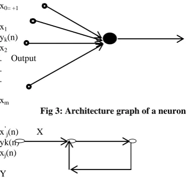
A neural network is a directed graph mainly expressed with nodes, with interconnecting synaptic and activation links. Block diagram provides a functional description of an individual network. The signal-flow graphs arrange a complete description of the signal flow in the network. Hence a signal-flow graph can be attained from an architectural graph describing the network formation. Feedback is said to exist in a dynamic system. Whenever the output of an element in the system influences a part of the input applied to that particular element, thereby giving rise to one or more closed pathsfor the transmission of signals,feedback is said to be generated around the system. Thus it plays a vital role in the study of a special class of neural networks known as the recurrent networks. Fig4. shows the signal-flow graph of a

single-loop feedback system, where the input signal xj(n),internal signal x‟j(n) and output signal yk(n) are functions

of discrete-time variable n. The system is assumed to be linear,consisting of a forward path and a feedback path that are characterized by the “operators” X and Y respectively. In particular, the output of the feedforward channel determines its own output through the feedback channel partly. From fig 3.2 the input-output relationships can be noted:

yk(n)=X[x‟j(n)] (3.1)

x0= +1

x1

yk(n)

x2

. Output .

.

[image:2.595.316.501.186.365.2]

xm

Fig 3: Architecture graph of a neuron

x‟j(n) X

yk(n) xj(n)

Y

Fig 4: Signal flow graph of a single loop feedback system

x‟j(n)= xj(n)+Y[yk(n)] (3.2)

where square brackets are included to emphasize that X and Y act as operators. Eliminating x‟j(n) between equations(3.1)and

(3.2),the value obtained is

yk(n)= [X/(1-XY)] xj(n) (3.3)

[X/(1-XY)] is referred as the closed-loop operatorof the system, and to XY as the open-loop operator. In general, the open-loop operator is non-commutative in that YX≠XY. Consider, the single-loop feedback system shown in Fig 5, for which X is a fixed weight; and Y is a unit delay operator z-1, whose output is delayed with respect to input by unit time. The closed-loop operator of the system is expressed as [X/ (1-XY)]= [w/ (1-wz-1)] =w (1-wz-1)-1

Using the binomial expansion for w(1-wz-1)-1, the closed loop operator of the system is written as

X/ (1-XY)=w ∞ 𝑤𝑙_𝑧−𝑙

𝑙=0 (3.4)

Hence, substituting Eq. (3.4) in (3.3), yk(n)=w 𝑤𝑙𝑧−𝑙

∞

𝑙=0 [xj(n)] (3.5)

Where again square brackets are used to emphasize the fact that z-1 is an operator .In particular from the definition of z-1

z-l[xj(n)]=xj(n-l) (3.6)

Where xj(n-l)is a sample of the input signal delayed by l time

units. Accordingly, the output signal yk(n)as is expressed as

an infinite weighted summation of present and past samples of the input signal xj(n),as shown by

yk(n)= ∞𝑙=0 𝑤𝑙+1xj(n-l) (3.7)

x‟j(n) w

G(s)

xj(n) yk(n)

[image:3.595.90.250.69.114.2]

z-1

Fig 5: Signal-flow graph of a first-order, infinite-duration impulse response (IIR) filter[9]

4.

SIMULATIONS AND MATLAB

CODING: BLOCK SET

REPRESENTATIONS WITH RESULT

ANALYSIS

4.1 Algorithm

Step 1: Initialize the values of the input (A) by rounding it to the random nearest integer value.

Step 2: Initialize the values of the target (B) with respect to the input function.

Step 3:.The hidden layers commonly have „tansig‟ transfer function (default for „newelm‟) and„logsig‟ is commonly the output layer transfer function.

Step 4: The input and the output sequence to be presented is again recalled to a network in cell array form.

Step 5: The function „train‟ is used to train an Elman network. Step 6: The output of the network is found with the function „sim‟.

Step 7: The output is convertedback to the concurrent form. Step 8: The difference between the target output and the simulated network output is calculated[10].

4.1.1

Flowchart approach

Fig 6: Flow chart approach of the algorithm

In this paper, from the block diagram representation the signal flow graph is obtained similar to Fig 5 which is later on implemented by neural networks in MATLAB (R2008b).

4.2

MATLAB Coding Approach Towards SFG

Incorporating With ANN

A= round (rand (1, 8)) %Randomize the values of the input B= [0 (A(1:end-1)+A(2:end) == 2)] %Compute the target values.

net = newelm(A,B,5,{'tansig','logsig'}) %Convert the sequence to cell array structure Aseq = con2seq (A)

Bseq = con2seq (B) %Train the network net = train(net,Aseq,Bseq)

%Compute the output of the network X = sim(net,Aseq)

y = seq2con(X) y{1,1}

diff1 = B - y {1, 1}

4.3

Result Analysis And Remarks on

Simulation Aspects

• A=

Columns 1 through 8 1 1 0 1 1 0 0 1

• B=

Columns 1 through 8 0 1 0 0 1 0 0 0 Random input values(A)are entered and the target(B) is set on the basis of the input. Here Bis defined to be 0, except when two 1's occur in A, in which case B is 1.The input and the output forms are then converted into cell array form.

The command “net” = “newelm (A, B,5,{'tansig','logsig'})” determines the number of hidden neurons (here 5)and „tansig‟neurons in its hidden (recurrent) layer, and „logsig‟ neurons in its output layer.

 X=

Columns 1 through 2 [0.5003] [0.9984] Columns 3 through 4 [0.5000] [0.5001] Columns 5 through 6 [0.9878] [0.5000] Columns 7 through 8 [0.5001] [0.5000]

 y{1,1} ans =

Columns 1 through 3 0.5003 0.9984 0.5000 Columns 4 through 6 0.5001 0.9878 0.5000 Columns 7 through 8 0.5001 0.5000

 diff1 =

Columns 1 through 3 -0.5003 0.0016 -0.5000 Columns 4 through 6 -0.5001 0.0122 -0.5000 Columns 7 through 8 -0.5001 -0.5000

After training, the network is simulated with the input Aand the difference between the target output is calculated and the simulated network output. As the difference obtained between the target and the simulated output of the trained network is very small it is determined that the network is trained correctly.

The otherinformation obtained from the program coding: Start

Enter the input values

Enter the target values

i/p& o/p values presented in a cell-array format

Declare the function to create Elman network

Train the network

Find the o/p of the function

Convert the o/p back in the concurrent form

Calculate the difference b/t the target and the network o/p

Target ≈simulated o/p

End process

[image:3.595.37.293.419.755.2]

•„numInputs‟: 1,„numLayers‟: 2:It is the number of input and layer sources, not the number of elements in an input vector.

„biasConnect‟:[1; 1],„input Connect‟:[1; 0],layer Connect‟:[1 0; 1 0],output Connect‟: [0 1]:The bias connection matrix is a 2-by-1 vector. The input connection matrix is 2-by-1, representing the presence of connections from the sources (the input) to two destinations.Similarly this 2-by-2 matrix represents the presence of a layer and the output connections are a 1-by-1 matrix, indicating that they connect to one destination (the external world) from two sources (the two layers).

• „numOutputs‟: 1:By defining output connection, it is specified that the network has one output. • „numInputDelays‟: 0,numLayerDelays‟: 1: It

represents the number of input and layer delays in the network.

• „biases‟: {2x1 cell} „inputs‟: {1x1 cell}

,

„layers‟: {2x1 cell},outputs‟: {1x2 cell}: The structure of the given matrix format is automatically updated with respect to the givenbias,input, layer and output commands.

• „input Weights‟: {2x1 cell}, layer Weights‟: {2x2 cell}: containing 1 input weight and 2 layer weights. Each input weight has as many columns as the size of the input multiplied by the number of its delay values.

• „adaptFcn‟: „trains‟: This sets „net.adaptParam‟ to „trains's‟ default parameters.

• „divideFcn‟: 'dividerand': This set the divide function to dividerand (divide training data randomly).

• „gradientFcn‟: 'calcgrad': The gradient function is set using „calcgrad‟ in order to calculate the gradient of the network. This gradient is actually an approximation, because the contributions of weights and biases to errors via the delayed recurrent connection are ignored and it is then used to update the weights with the chosen backpropagation training function. The function „traingdx‟ is recommended.

• „initFcn‟: „initlay‟: Set the initialization function to „initlay‟ so the network initializes itself according to the layer initialization functions already set to „initnw‟,(the Nguyen-Widrow initialization function) meeting the initialization requirement of the network.

• „performFcn‟:'mse',trainFcn‟: 'traingdx':The performance function is set to „mse‟ (mean squared error) and the training function to „traingdx‟ to meet the final requirement of the network.

• „plotFcns‟: „{'plotperform','plottrainstate'}‟: Plot functions areset to „plotperform‟ and „plottrainstate‟•„adaptParam‟:„.passes‟,

• „divideParam‟: „.trainRatio‟, „.valRatio‟, „.testRatio‟

• „gradientParam‟ :( none),

„initParam‟:(none),„performParam‟: (none)

• These parameters must be displayed in order to show the different parameters of the network. • •„trainParam‟:„.show‟,„.showWindow‟,

.showCommandLine‟, „.epochs‟,„.time‟,„.goal‟, „.max_fail‟, „.lr,.lr_inc‟,„.lr_dec‟, „.max_perf_inc‟, „.mc‟, „.min_grad‟

• The training parameters must be prepared to display the different values associated with the training of the network. Training launches the neural network training windowFig(6)

• „IW‟ :{ 2x1 cell}, „LW‟: {2x2 cell}, „b‟: {2x1 cell}: containing 1 input and2 layer weight matriceswith 2 bias vectors. These cell arrays contain weight matrices and bias vectors in the same positions that the connection properties contain 1's and the sub object properties contain structures.

• Other:„name‟: '' „userdata‟: (user information)

From the above outputs the pictorial representation of the neural network is also obtained which shows the

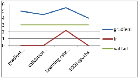
[image:4.595.314.540.438.564.2]

1) Algorithms including Training (Gradient Descent Backpropagation with Adaptive Learning rate), Performance (Mean Squared Error-mse) and Data Division (Random-Dividerand).

Table 1: Progress of the network

Progress Values Range

1. Epoch 1000 iterations 0-1000

2. Time 0:00:13 ---

3. Performance 0.188 0.437-0.000

4. Gradient 3.60e-.08 1.00-(1.00e-10)

5.Validation checks 0 0-6

2) Plot showing Performance (plotperform) and Training state (plottrainstate)

Fig7: The above figure shows the training state

Thus, it can be concluded that proper result is obtained after proper coding and the graphs obtained determines that the program has run successfully.Since the input values are randomly considered it can change each time with the coding and hence the results can vary accordingly. This coding is done in such a manner that it will help any user (even a beginner) universally to access the codes easily.

network are depicted at different points in time are similar or dissimilar.The resultsreported here suggest that these networks have appreciable representational potentialwith moresystematic analysis using better defined tasks which is clearly desirable [11].

For an Elman network to have the highest chance at learning a problem, it needs more hidden neurons in its hidden layer than are actually required for a solution by another method. Whereas a solution might be available with fewer neurons, the Elman network is less efficient to find the most appropriate weights for hidden neurons because the error gradient is approximated. Therefore, having a considerable number of neurons to begin with makes it more acceptable that the hidden neurons will start out dividing up the input space in different useful manners [12].

5.

TRADITIONAL MODELING

APPROACH TO ADVANCE ANN

DESIGN ACCESION: COMPARATIVE

STUDY

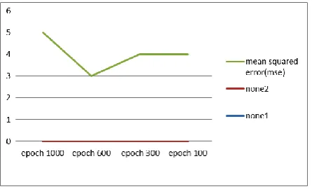
This study examines the performance of a control block with a combination of both feedforward/feedback represented with an ANN model. In the simulation process, demonstration of the clear superiority of the ANN design over the normal approach is determined. In this paper the feedback in a control system is discussed with and without ANN.Elman neural network with its sequential inputs are built and employed in the paper, with a result that the ANN model makes perform significantly better than the ordinary control block.

Fig 8: The above figure shows the performance of a trained neural network with the plot (‘mse’vs ‘epoch’)

[image:5.595.54.277.430.565.2]

showing the best training performance in epoch 205

Table 2: Comparative study of ANN with Traditional Control Block

SL No.

Transfer functions

ANN Design o/p

Control block o/p

Accuracy of ANN by difference

1. G(s)=(5/s2+3s+5) [3 3 5] [0 0 1] [-2 0 0] 2. G(s)=(1/s2+3s +s) [2 3 2] [0 0 1] [-1 0 -1] 3. G(s)=(3s/s2+3s+5) [3 3 5] [0 1 0] [-2 0 0] 4. G(s)=(s+3/s2+3s+5) [3 3 5] [0 .3 .6] [-2 0 0]

To strengthen practical experience in applying ANN-based control block modeling, a detailed procedure of the coding is

also documented

.

6. CONCLUSION

In this paper a way of implementation of a control block into artificial neural networks using MATLAB(R2008b).The prospect of this paper is to help the researchers to implement any transfer function into artificial neural network in different fields of study.The control system and artificial neural network collectively find huge application in the fields of neural computing,control of dynamical systems using artificial neural network,application of feedback and feedforward network etc.Hence for this it can become a very effective aspect globally for artificial neural networks and control system altogether.

7. ACKNOWLEDGEMENTS

Thanks to MATLAB(R2008b) who have contributed towards

development of this paper

.

8. REFERENCES

[1] U.A. Bakshi,V.UBakshi, „Principles of Control Systems‟, First Edition,pp-(4-1),T.Publications Pune, 2009

[2]Ricardo Perussi-e-Silva, ViniciusOliverio, Julio Cesar Rosa-e-Silva, Francisco Jose Candido-dos- Reis, Antonio Alberto Nogueira, OmeroBenedictoPoli-Neto,„The Importance of Computing Systems in Chronic Pelvic Pain Research,International Journal of Computer and Information Technology‟,Volume 02,pp-(258), 02, March 2013

[3]Woo Chaw Seng, MahsaChitsaz,„Handgrip Strength Evaluation UsingNeuro FuzzyApproach‟,Malaysian Journal of Computer Science, Vol. 23(3),pp-(167), 2010

[4]Simon Haykin, „Neural Networks and learning machines‟, Volume 10,pp.-(15),Prentice Hall, 2009.

[5] John Doyle, Bruce Francis, Allen Tannenbaum “Feedback Control Theory”,Macmillan Publishing Co., pp-01-02, 1990.

[6]S.K.Bhattacharya,Linear control systems:ForPTU,pp-(51-52),D.K(India)PvtLmt,Pearson Education,2011

[7] U.A. Bakshi, V.U Bakshi, „Automatic Control Systems‟, First Edition,pp- (6-2),T.Publications Pune,2009

[8]Norman S.Nise, „Control Systems Engineering‟,FourthEdition,pp-(258,267),John Wiley & Sons(Asia)Pte.Ltd,2004

[9] Simon Haykin, „Neural Networks:A Comprehensive Foundation‟, 2nd Edition,pp-(39-41),Pearson Education,2005

[10] Lishan Kang, XuesongYan,„Advances in Computation and Intelligence: Third International Symposium on Intelligence Computation and Applications‟,pp-(319), Springer –Verlag B H, 2008

[11]JeffreyL.Elman,„Finding Structure in Time,Cognitive Science‟, Vol. 14,pp-(24,25), 1990