POPULATION DYNAMICS PROBLEM
OUMAR TRAOREReceived 23 November 2005; Revised 8 August 2006; Accepted 11 October 2006
We establish a null controllability result for a nonlinear population dynamics model. In our model, the birth term is nonlocal and describes the recruitment process in newborn individuals population. Using a derivation of Leray-Schauder fixed point theorem and Carleman inequality for the adjoint system, we show that for all given initial density, there exists an internal control acting on a small open set of the domain and leading the population to extinction.
Copyright © 2006 Hindawi Publishing Corporation. All rights reserved.
1. Introduction
For a given positive real functionF, we consider in this paper the following nonlinear population dynamics model:
∂y ∂t +
∂y
∂a−Δy+μy=v1ω in (0,T)×(0,A)×Ω, y(t,a,σ)=0 on (0,T)×(0,A)×∂Ω,
y(0,a,x)=y0(a,x) in (0,T)×(0,A)×Ω,
y(t, 0,x)=F A
0 β(t,a,x)y(t,a,x)da
on (0,T)×Ω,
(1.1)
whereΩis a bounded open subset ofRN,N≥1 with a smooth boundary∂Ω,σ∈∂Ω, T is a positive real and ω an open subset such that ω⊂Ω. Here y(t,a,x) is the dis-tribution of individuals of ageaat timet and locationx ∈Ω, 1ω is the characteristic function of ω,A is the maximal live expectancy, Δthe Laplacian with respect to the spatial variable,β(t,a,x) andμ(t,a,x) denote, respectively, the natural fertility and the natural death rate of individuals of ageaat timetand location x. Thus, the formula A
0 β(t,a,x)y(t,a,x)dadenotes the distribution of newborn individuals at timetand loca-tionx. In an oviparus species it denotes the total eggs at timetand positionx. Therefore, the quantityF(0Aβ(t,a,x)y(t,a,x)da) is the distribution of eggs that hatches at timet and positionx.
Hindawi Publishing Corporation
International Journal of Mathematics and Mathematical Sciences Volume 2006, Article ID 49279, Pages1–20
System (1.1) describes the evolution of an internal controlled age and space structured population under inhospitable boundary conditions in the case that the flux of individu-als has the form−∇y(t,a,x).
The purpose of this paper is to prove a null controllability result for (1.1) at any time T. This means more precisely that there exists a controlv∈L2((0,T)×(0,A)×ω) such that the associated solution of (1.1) verifies
y(T,a,x)=0 a.e. in (0,A)×Ω. (1.2)
In our knowledge the first controllability result for an age and space structured popu-lation dynamics model was established by Ainseba and Langlais in [4]: they proved that a set of profiles is approximately reachable. In [2] a local exact controllability result was proved for a linear population dynamics. More precisely, in [2] the authors proved that if the initial distribution is small enough, one can find a control that leads the population to extinction. The method used there is different from ours. In fact in [2] the adjoint system was taken as a collection of parabolic equations along characteristic lines. This allowed the authors to use Carleman inequality for parabolic equation. Ainseba and Iannelli in [3] proved a null controllability result for a nonlinear population dynamics model. In [3] the natural rates depend on the total populationP=0Ay(t,a,x)da. The method in [3] used Kakutani fixed point theorem. Therefore, crucial assumptions were made: first, the natural rates were supposed to be globally Lipschitz with respect to the variableP, secondly in order to perform key estimates, the death rateμverified the following growth condition: 0≤μexp(0aμ(s)ds)≤ζwhereζis a positive constant.
In the case we study here, the above results cannot be applied. Indeed, since the birth process is not globally Lipschitz with respect to the variablePand, without the previous growth condition onμone cannot use the method of [3]. On the other hand, the nonlin-earity excludes the use of the result of [2]. In what follows, using a Carleman inequality for an adjoint system we establish a null controllability result for the nonlinear popula-tion dynamics models stated in (1.1) when the initial distribution is inL2((0,A)×Ω). Roughly, in our method we first study a null controllability result for a population in which the birth process is given by a fixed function. Afterwards, we prove the null con-trollability result for the system (1.1) by means of a derivation of Leray-Shauder theorem. The remainder of this paper is as follows: inSection 2, we state assumptions and we provide the main result. InSection 3we study a null controllability result for some asso-ciated model.Section 4is devoted to the proof of the main result.
2. Assumptions and main result
For the sequel we assume that the following assumptions hold:
H1 ⎧ ⎪ ⎪ ⎪ ⎪ ⎪ ⎪ ⎪ ⎨ ⎪ ⎪ ⎪ ⎪ ⎪ ⎪ ⎪ ⎩
μ(t,a,x)=μ0(a) +μ1(t,a,x) a.e. in (0,T)×(0,A)×Ω, μ≥0 a.e. in (0,T)×(0,A)×Ω,
μ1∈L∞
(0,T)×(0,A)×Ω; μ1(t,a,x)≥0 a.e. in (0,T)×(0,A)×Ω, μ0∈L1loc(0,A), lima→A
a
H2 ⎧ ⎪ ⎪ ⎪ ⎪ ⎪ ⎨ ⎪ ⎪ ⎪ ⎪ ⎪ ⎩
β∈C2[0,T]×[0,A]×Ω,
β(t,a,x)≥0 in [0,T]×[0,A]×Ω,
∃0< a0< a1< A such thatβ(t,a,x)=0 in [0,T]×
0,a0
a1,A×Ω.
(2.1)
H3Fdefined onRis a positive continuous function and there exist positive constantsC0 andC1such thatF(t)≤C0+C1|t|, for allt∈R.
Remark 2.1. Since μ and β are natural rates, the second assumptions of H1 and H2 are natural. The third assumption ofH2 is also natural, since it means that older and younger individuals are not fertile. The fourth assumption inH1is also a standard one, it means that all individual dies before the ageA. In [3] the model did not take explic-itly into account the death of newborns. Indeed the birth process there has the form y(t, 0,x)=0Aβ(t,a,x,P(t,x))y(t,a,x)dawhereP(t,x)=
A
0 y(t,a,x)da. We present here a quite different model. In fact our model addresses both supply and death of newborns. Moreover in the caseF(t)=ktwithka fixed positive constant, one obtains from (1.1) a linear population dynamics problem.
Assume now that the functionFis a globally Lipschitz one and verifiesF(0)=0. Then, one can rewriteF asF(t)=tΦ(t) for a.e.t∈R. Therefore, the fourth equation of (1.1) becomesy(t, 0,x)=0Aβy daΦ(
A
0 βy da). Hence, one obtains the system considered with Neumann boundary conditions in [8,10] where existence of solution was studied.
From now we setQ=(0,T)×(0,A)×Ω; q=(0,T)×(0,A)×ω;QA=(0,A)×Ω; QT=(0,T)×Ω;Σ=(0,T)×(0,A)×∂ΩandCβ= βC2(Q).
Forα≥0 we setSα(t,a)=exp(−αt+0aμ0(s)ds),Xα= {z∈L2(QA);Sα(t,a)z∈L2(QA)}, andYα= {v∈L2(q); Sα(t,a)v∈L2(q)}. It is obvious thatα1≥α2impliesXα1⊂Xα2and Yα1⊂Yα2.
In the sequel,νwill denote the unit outward normal vector to∂ΩandC(Ω,T,A,. . .) will denote positive constant that depends only onΩ,T,A,. . . .
We are now ready to state the main result of this paper.
Theorem 2.2. For anyγ >0 assumed to be small enough, there exists a controlv∈Y0such that the associated solution of (1.1) satisfies
y(T,a,x)=0 a.e. in (γ,A)×Ω (2.2)
for ally0∈X0.
Remark 2.3. In the proof, it will appear clearly that such a control depends essentially onγ.
Let us denote byλ0a positive constant which will be fixed later. We make the following standard changes:y=Sλ0(t,a)y,v=Sλ0(t,a)v,β=S−
1
it follows thatysolves the following system:
∂y ∂t +
∂y ∂a−Δy+
μ1+λ0
y=v1ω inQ,
y(t,a,σ)=0 onΣ,
y(0,a,x)=y0(a,x) inQA,
y(t, 0,x)=e−λ0tF
eλ0t A
0
β(t,a,x)y(t,a,x)da
inQT.
(2.3)
The null controllability problem ofTheorem 2.2is now reduced to findvinL2(q) such thatyverifies (2.2). In fact after the previous change we obtain a system involving bound-ed coefficients and this allows one to establish a global Carleman inequality. In the sequel for the sake of simplicity, we will consider only the previous system without hats and in addition we will writeμinstead ofμ1+λ0.
3. Null controllability for some linearized model
3.1. An observability inequality result. We recall here that there exists a functionΨ∈ C2(Ω) such thatΨ(x)=0, for allx∈∂Ω;Ψ(x)>0, for allx∈Ωand∇Ψ(x)=0, for all x∈Ω−ωwhereωis an open set such thatω⊂ω⊂Ω. (See [6] for the existence ofΨ.)
Let us consider the following system:
−∂w
∂t − ∂w
∂a−w+μw=f inQ, w(t,a,σ)=0 onΣ,
w(T,a,x)=g(a,x) inQA, w(t,A,x)=0 inQT.
(3.1)
Setting for all positive realλ,η(t,a,x)=(e2λΨ∞−eλΨ(x))/at(T−t) andϕ(t,a,x)=eλΨ(x)/ at(T−t) one can prove easily by adapting the method of [6] or [9] the following.
Proposition 3.1. There exist positive constantss1≥1 andλ1≥1 and there exists a pos-itive constantCsuch that for alls≥s1,λ≥λ1, and for all solution of (3.1), the following inequality holds:
Qe
−2sηs3ϕ3λ4w2dt da dx≤C
Qe
−2sηf2dt da dx+
qe
−2sηs3ϕ3λ4w2dt da dx
. (3.2)
Remark 3.2. The proof ofProposition 3.1is absolutely similar to those of global Carleman inequality for the linear heat equation proposed in [9] or in [6]. Roughly, for the proof of (3.2), one makes the change of variable:u=e−sηwin order to get from the definition of ηthe following:
u(0,a,x)=u(T,a,x)=u(t, 0,x)=0. (3.3)
Proof ofProposition 3.1. We suppose that the functionw∈C2(Q) and verifies (3.1) and we make the following change of variablesu=e−sηw. Then immediately it follows by using the definition ofηand (3.1) that
u(0,a,x)=u(T,a,x)=0 in (0,A)×Ω, (3.4)
u(t, 0,x)=u(t,A,x)=0 in (0,T)×Ω, (3.5)
u(t,a,σ)=0 in (0,T)×(0,A)×∂Ω. (3.6)
Notice that
∇η= −λϕ∇Ψ, (3.7)
∇ϕ=λϕ∇Ψ. (3.8)
Using once again the definitions ofηandϕ, we deduce that there exist positive constants denoted byCsuch that|∂η/∂a| ≤Cϕ2,|∂η/∂t| ≤Cϕ2,|∂2η/∂a∂t| ≤Cϕ3, and|∂η/∂a2| ≤ Cϕ3.
Similarly we get
∂ϕ∂a≤Cϕ2, ∂ϕ ∂t
≤Cϕ2, ∂ 2ϕ ∂a∂t
≤Cϕ3, ∂ϕ ∂a2
≤Cϕ3. (3.9)
We have
∂u ∂t +
∂u ∂a= −s
∂η
∂t + ∂η ∂a
u+e−sη ∂w
∂t + ∂w
∂a
. (3.10)
From (3.7) and (3.8) we get
Δu=sλΔΨϕu+sλ2|∇Ψ|2ϕu−s2λ2|∇Ψ|2ϕ2u+ 2sλϕ∇Ψ· ∇u+e−sηΔw. (3.11)
Therefore
−
∂u ∂t +
∂u ∂a
−Δu+μu
=e−sηf−sλ2uϕ|∇Ψ|2−2sλϕ∇Ψ· ∇u+s2λ2ϕ2|∇Ψ|2u+s∂η ∂t +
∂η ∂a
u−sλϕuΔΨ. (3.12)
This equation can be rewritten as
P1u+P2u=gs, (3.13)
where
P1u= −∂u ∂t −
∂u
∂a+ 2sλϕ∇Ψ· ∇u+ 2sλ
2uϕ|∇Ψ|2,
P2u= −Δu−s ∂η
∂t + ∂η ∂a
u−s2λ2ϕ2|∇Ψ|2u,
gs=e−sηf+sλ2uϕ|∇Ψ|2−μu−sλuϕΔΨ.
Taking the square of (3.13) and integrating the result overQyield
Q P1u2
dt da dx+
Q P2u2
dt da dx+ 2
QP2uP1u dt da dx=
Qg 2
sdt da dx. (3.15)
Let us computeK=QP2uP1u dt da dx. We obtain
K=
Q
−∂u
∂t − ∂u
∂a+ 2sλϕ∇Ψ· ∇u+ 2sλ
2uϕ|∇Ψ|2
−Δu−s ∂η
∂a+ ∂η
∂t
u
dt da dx
−
Q
−∂u
∂t − ∂u
∂a+ 2sλϕ∇Ψ· ∇u+ 2sλ
2uϕ|∇Ψ|2s2λ2ϕ2|∇Ψ|2u dt da dx.
(3.16)
This computation gives twelve terms denoted byIi,j,i=1,. . ., 4, j=1, 2, 3. We have by integration by parts
I1,1=
Q ∂u
∂tΔudt dadx=
Σ ∂u ∂t
∂u
∂νdt da dσ− 1 2
Q ∂ ∂t|∇u|
2dt da dx. (3.17)
Hence using (3.4) and (3.6) it follows that
I11=0,
I1,2=s
Q ∂u
∂t ∂η
∂a+ ∂η ∂a
u dt da dx. (3.18)
An integration by parts leads to
I1,2= −s 2
Q|u| 2 ∂
∂t ∂η
∂a+ ∂η ∂a
dt da dx,
I1,3=s2λ2
Q ∂u
∂tϕ
2u|∇Ψ|2dt da dx.
(3.19)
This gives
I1,3=s 2λ2
2
Q ∂|u|2
∂t ϕ
2|∇Ψ|2dt da dx. (3.20)
Keeping in mind (3.4), an integration by parts with respect to the variabletyields
I1,3= −s2λ2
Q|u| 2∂ϕ
∂tϕ|∇Ψ|
Similarly, one gets easily that
I21=0,
I2,2= − s 2
Q|u| 2 ∂ ∂a ∂η ∂a+ ∂η ∂a
dt da dx,
I2,3= −s2λ2
Qϕ|u| 2∂ϕ
∂a|∇Ψ|
2dt da dx.
(3.22)
Now, we are concerned by the termI3,j. We have
I3,1= −2sλ
Qϕ∇Ψ· ∇uΔudt dadx. (3.23)
Then we have by an integration by parts
I3,1= −2sλ
Σϕ∇Ψ· ∇u ∂u
∂νdt da dσ+ 2sλ
Q∇u· ∇(ϕ∇Ψ· ∇u)dt da dx. (3.24) From the definition ofΨand since (3.6) is fulfilled we see that for allσ∈∂Ωwe have
∇u(t,a,σ)=(∇u(t,a,σ)·ν(σ))ν(σ) and∇Ψ(σ)=(∇Ψ(σ)·ν(σ))ν(σ). Therefore it follows, using also (3.8), that
I3,1= −2sλ
Σϕ(∇Ψ·ν)|∇u·ν|
2dt da dσ+ 2sλ2
Q|∇u· ∇Ψ|
2ϕ dt da dx
+ 2sλΣNi,j=1
Qϕ ∂u ∂xi
∂2u ∂xi∂xj
∂Ψ
∂xjdt da dx+
Qϕ ∂u ∂xi
∂2Ψ ∂xi∂xj
∂u
∂xjdt da dx
.
(3.25)
We have
2sλΣN i,j=1
Qϕ ∂u ∂xi
∂2u ∂xi∂xj
∂Ψ ∂xj
dt da dx
=sλ
Σϕ(∇Ψ·n)|∇u·n|
2dt da dσ−sλ2
Q|∇u|
2|∇Ψ|2ϕ dt da dx
−sλ
Qϕ|∇u|
2ΔΨdt dadx.
(3.26)
Therefore
I3,1= −sλ
Σϕ(∇Ψ·n)|∇u·ν|
2dt da dσ+ 2sλ2
Q|∇u· ∇Ψ|
2ϕ dt da dx
−sλ2
Q|∇u|
2|∇Ψ|2ϕ dt da dx−sλ2
Q|∇u|
2|∇Ψ|2ϕ dt da dx
−sλ
Qϕ|∇u|
2ΔΨdt dadx+ 2sλΣN i,j=1
Qϕ ∂2Ψ ∂xi∂xj
∂u ∂xj
∂u
∂xidt da dx
I3,2= −2s2λ
Qϕ∇Ψ· ∇u ∂η
∂t + ∂η ∂a
u dt da dx.
Classical computations give
I3,2= −s2λ2
Qϕ|∇ψ|
2|u|2∂η ∂t +
∂η ∂a
dt da dx+s2λ
Qϕ|u|
2∇ ·∇Ψ∂η ∂t +
∂η ∂a
,
I3,3= −2s3λ3
Qϕ
3∇Ψ· ∇u|∇Ψ|2u dt da dx.
(3.28)
Equality (3.8) and an integration by part give
I3,3=3s3λ4
Qϕ
3u2|∇Ψ|4dt da dx+s3λ3
Qϕ
3|u|2∇ ·∇Ψ|∇Ψ|2dt da dx. (3.29)
Now we compute the termsI4,j
I4,1= −2sλ2
Qϕu|∇Ψ|
2Δudt dadx=2sλ2
Q∇
ϕu|∇Ψ|2· ∇u dt da dx. (3.30)
Therefore
I4,1=2sλ3
Qϕu∇Ψ· ∇u|∇Ψ|
2dt da dx+ 2sλ2
Qϕ|∇u|
2|∇Ψ|2∇u dt da dx
+ 2sλ2
Qϕu∇u· ∇
|∇Ψ|2dt da dx.
(3.31)
Directly, we have
I42= −2s2λ2
Qϕ|∇Ψ| 2
∂η
∂t + ∂η ∂a
|u|2dt da dx, (3.32)
I43= −2s3λ4
Qϕ
3|∇Ψ|4u2dt da dx. (3.33)
Grouping all the termsIi,jand using the boundeness of the derivatives ofϕandηone can write
2
QP1uP2u dt da dx=X1+X2−2sλ
Σϕ∇Ψ·ν|∇u·ν|
2dt da dσ
+ 4sλ2
Qϕ|∇u· ∇Ψ|
2dt da dx
+ 2sλ2
Qϕ|∇u|
2|∇Ψ|2dt da dx+ 2s3λ4
Qϕ
3u2|∇Ψ|4dt da dx, (3.34)
whereX1andX2verify
X1≤C
sλ+λ2 Qϕ|∇u|
2dt da dx,
X2≤C
s2λ4+s3λ3 Qϕ
3|u|2dt da dx.
Note thatνis the outward normal vector to∂Ω. So, using the fact thatΨ(x)>0 for all x∈ΩandΨ(σ)=0 for allσ∈∂Ωwe infer that∇Ψ·ν<0. Therefore, (3.34) yields
2
QP1uP2u dt da dx≥X1+X2+ 2sλ 2
Qϕ|∇u|
2|∇Ψ|2dt da dx
+ 2s3λ4
Qϕ
3u2|∇Ψ|4dt da dx.
(3.36)
Note also thatΨ∈C2(Ω) and|∇Ψ| =0 inΩ−ω. Consequently, there exists a positive constantδsuch that|∇Ψ|> δinΩ−ω. Therefore (3.36) gives
2
QP1uP2u dt da dx+ 2sλ 2δ2
qϕ|∇u|
2dt da dx+ 2s3λ4δ4
qϕ
3u2dt da dx
≥X1+X2+ 2sλ2δ2
Qϕ|∇u|
2dt da dx+ 2s3λ4δ4
Qϕ
3u2dt da dx,
(3.37)
whereq=(0,T)×(0,A)×ω. Furthermore, we have
Qg 2
sdt da dx≤
Qe
−2sηf2dt da dx+X
1+X2. (3.38)
Then, it follows from (3.15) and (3.37) that
Qe
−2sηf2dt da dx+X
1+X2+ 2s3λ4δ4
qϕ
3|u|2dt da dx+ 2sλ2δ2
qϕ|∇u|
2dt da dx
≥
Q P1u2
dt da dx+
Q P2u2
dt da dx+ 2sλ2δ2
Qϕ|∇u|
2dt da dx
+ 2s3λ4δ4
Qϕ
3|u|2dt da dx.
(3.39)
We can choosesandλsufficiently large so that
sλ2δ2
Qϕ|∇u|
2dt da dx+s3λ4δ4
Qϕ
3|u|2dt da dx≥X
1+X2. (3.40)
This means more precisely that there exists positive constantss1>1 andλ1>1 such that fors≥s1andλ≥λ1(3.39) yields
Qe
−2sηf2dt da dx+ 2s3λ4δ4
qϕ
3|u|2dt da dx+ 2sλ2δ2
qϕ|∇u|
2dt da dx
≥
Q P1u2
dt da dx+
Q P2u2
dt da dx+sλ2δ2
Qϕ|∇u|
2dt da dx
+s3λ4δ4
Qϕ
3|u|2dt da dx.
We want now to eliminate the term
2sλ2δ2
qϕ|∇u|
2dt da dx (3.42)
in (3.41). For this aim, we introduce a cut-offfunctionαsuch thatα∈C∞0(ω); 0≤α≤1; andα=1 onω.
MultiplyingP2ubyϕα2uand integrating the result overQleads to
Qϕα 2uP
2u dt da dx
= −s
Q ∂η
∂t + ∂η ∂a
u2ϕα2dt da dx−s2λ2
Qu
2ϕ3α2|Ψ|2dt da d−
QuΔuϕα
2dt da dx. (3.43)
Note that
QuΔuϕα
2dt da dx
= −
Q|∇u|
2ϕα2dt da dx−λ
Qu∇u· ∇Ψϕα
2dt da dx−2
Qu∇u· ∇αϕα dt da dx. (3.44)
Therefore
Qϕα 2uP
2u dt da dx= −s
Q ∂η
∂t + ∂η ∂a
u2ϕα2dt da dx
−s2λ2
Qu
2ϕ3α2|Ψ|2dt da dx+
Q|∇u|
2ϕα2dt da dx
+λ
Qu∇u· ∇Ψϕα
2dt da dx+ 2
Qu∇u· ∇αϕα dt da dx. (3.45)
This gives
Q|∇u|
2ϕα2dt da dx=
Qϕα 2uP
2u dt da dx+s
Q ∂η
∂t + ∂η ∂a
u2ϕα2dt da dx
+s2λ2
Qu
2ϕ3α2|Ψ|2dt da dx−λ
Qu∇u· ∇Ψϕα
2dt da dx
−2
Qu∇u· ∇αϕα dt da dx.
(3.46)
Note that
−λ
Qu∇u· ∇Ψϕα
2dt da dx≤Cλ2
Q|u|
2ϕα2dt da dx+1 2
Q|∇u|
whereC is a positive constant. Asϕ≤Cϕ3 withC a positive constant, using now the properties ofαandΨwe deduce
q|∇u|
2ϕα2dt da dx
≤C
Qϕα 2uP
2u dt da dx+Cs2λ2
Qu
2ϕ3α2dt da dx+C
Quϕ
1/2|∇u|ϕ1/2α dt da dx. (3.48)
Therefore we deduce from the previous estimate that
2sλ2δ2
q|∇u|
2ϕ dt da dx≤1 2
Q
P2u2dt da dx+Cs2λ2
qu
2ϕ3dt da dx, (3.49)
whereCis a positive constant.
Combining (3.41) and (3.49) we get
C
Qe
−2sηf2dt da dx+s3λ4
qϕ
3u2dt da dx
≥
Q P1u2
dt da dx+
Q P2u2
dt da dx+sλ2
Qϕ|∇u|
2dt da dx
+s3λ4
Qϕ
3u2dt da dx.
(3.50)
We want now to turn back to the variablew. Note thatu=e−sηw. Then, we have
Qϕ
3|u|2dt da dx=
Qe
−2sηϕ3|w|2dt da dx,
qϕ
3|u|2dt da dx=
qe
−2sηϕ3|w|2dt da dx.
(3.51)
Therefore one gets from (3.50)
s3λ4
Qϕ
3e−2sηw2dt da dx≤C
Qe
−2sηf2dt da dx+Cs3λ4
qe
−2sηϕ3w2dt da dx.
(3.52)
This ends the proof.
of (3.1) the following inequality holds:
Q e−2sη
sϕ
∂w∂t +∂w ∂a
2+|Δw|2dx da dt+
Qe
−2sηs3ϕ3λ4w2dt da dx
+
Qe
−2sηsλϕ|∇w|2dt da dx≤C
Qe
−2sηf2dt da dx+
qe
−2sηs3ϕ3λ4w2dt da dx
.
(3.53)
It is sufficient to use (3.50) and to turn back to the variablewby using the explicit expres-sion ofP1uandP2u.
(ii) In [1] the author tried to prove a Carleman inequality for the system (3.1) with βw(t, 0,x) instead of f. The problem there is more complex: after the change of vari-ableu=e−2sηwthe right term becomese−2sηw(t, 0,x) and cannot be written in terms of the variableu. Unfortunately, see [1, system (6) page 566], this term was ignored in the computations.
In the sequel we take f =0 in order to avoid this situation.
Our observability inequality is as follows.
Proposition 3.4. Assume that
f =0 (3.54)
and that there exists a realγ≥0 such that
g(a,x)=0 a.e. in (0,γ)×Ω. (3.55)
Then, there exists a positive constantCγsuch that the following inequality holds:
QAw
2(0,a,x)da dx+
QTw
2(t, 0,x)dt dx≤C γ
qw
2(t,a,x)dt da dx (3.56)
for all solutionwof (3.1).
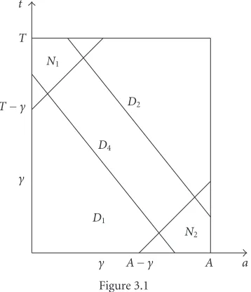
Letγbe small enough so thatγ≤min(T,A). We define now two subsets of (0,T)×
(0,A):
N1=
(t,a)∈(0,T)×(0,A); t≥a+T−γ,
N2=
(t,a)∈(0,T)×(0,A); t≤a+γ−A,
(3.57)
and we formulate a lemma which will be used in the proof ofProposition 3.4.
Lemma 3.5. If (3.54) and (3.55) hold, then all solutions of (3.1) verify
w(t,a,x)=0 a.e. inN1∪N2
Proof ofLemma 3.5. We will prove thatw=0 on almost every characteristic line inN1∪ N2.
Let (t0,a0)∈N1. Then we have t0=a0+T−γ+dwith 0≤d≤γ. Therefore,a0≤ γ−d.
LetS(d)= {(t0+s,a0+s), s∈(0,γ−d−a0)}be a characteristic line of (3.1). Setting z(s,x)=w(t0+s,a0+s,x) and μ(s,x)=μ(t0+s,a0+s,x) from (3.1), we deduce that z solves
−∂z
∂s− z+μz=0 in
0,γ−d−a0×Ω,
z(s,x)=0 on0,γ−d−a0
×∂Ω,
zγ−d−a0,x=w(T,γ−d,x)=g(γ−d,x) inΩ.
(3.59)
Then from (3.55) for almost alld∈(0,γ), standard results on heat equation imply that z=0. Thus, for almost alld∈(0,γ), w=0 onS(d). Therefore, w=0 inN1×Ω. The same argument and the fact thatw(t,A,x)=0 in (0,T)×Ωallow us to prove thatw=0
inN2×Ω.
Now, let us proveProposition 3.4.
Proof ofProposition 3.4. We set
D1=
(t,a)∈(0,T)×(0,A), t≤ −T−γ/2
A−γ/2a+T− γ 2
,
D2=
(t,a)∈(0,T)×(0,A), a≥ −A−γ/2
T−γ/2t+A−
γ(γ−2A) 2(2T−γ)
,
D3=(0,T)×(0,A)−
D1∪D2
,
D4=(t,a)∈D3; (t,a)∈/ N1∪N2, (cf.Figure 3.1).
(3.60)
Consider nowθ∈C0∞(R2) a cut-offfunction such that θ=1 on D1;θ=0 on D2. Settingw=θw, it follows thatwsolves
−∂w
∂t − ∂w
∂a −w+μw= − ∂θ
∂t + ∂θ ∂a
w inQ,
w(t,a,x)=0 onΣ,
w(T,a,x)=0 inQA,
w(t,A,x)=0 inQT.
(3.61)
Multiplying (3.61) bywand integrating overQyield after minor majoration T−γ/2
0
Ωw
2(t, 0,x)dx dt+ A−γ/2
0
Ωw
2(0,a,x)dx da≤ −2
Q ∂θ
∂t + ∂θ ∂a
γ A γ A a γ
T γ
T t
D1
N2
D4
D2
N1
Figure 3.1
UsingLemma 3.5and the definition ofθ, we deduce that (∂θ/∂t+∂θ/∂a)θw=0 almost every where outside of D4×Ω. Note that ηandϕare bounded on D4×Ωby strictly positive reals. Hence there exists a positive constantCγ>0 such that
−2
Q ∂θ
∂t + ∂θ ∂a
θw2dt da dx≤C γ
Qϕ
2e−2sηw2dt da dx. (3.63)
Therefore (3.62) yields
T−(γ/2)
0
Ωw
2(t, 0,x)dx dt+ A−(γ/2)
0
Ωw
2(0,a,x)dx da≤C γ
Qϕ
2e−2sηw2dt da dx, (3.64)
whereCγis a positive constant depending onγ. Using now (3.2), (3.58) and the fact that ϕ2e−2sη≤1 forλandssufficiently large we deduce (3.56). Remark 3.6. A careful calculation fors≥s1andλ≥λ1leads to the following estimate of Cγ:
Cγ≥C(T)γ2exp
C(Ψ,s,λ)
γ3AT
, (3.65)
[image:14.468.145.324.74.282.2]3.2. A null controllability result. In this section, for a given function b∈L2(Q T) we consider the following system:
∂y ∂t +
∂y
∂a−y+μy=v1ω inQ, y(t,a,σ)=0 onΣ,
y(0,a,x)=y0(a,x) inQA, y(t, 0,x)=b(t,x) inQT.
(3.66)
For all>0 we introduce the functional
J(v)=21
A
γ
Ωy
2(T,a,x)dx da+1 2
qv
2(t,a,x)dx da dt. (3.67)
It follows easily thatJ is continuous, convex, and coercive. Hence,J admits a unique
minimizervand we have
v(t,a,x)= −w(t,a,x)1ω(x) inQ, (3.68)
wherewis the solution of the following system:
−∂w
∂t − ∂w
∂a −Δw+μw=0 inQ, w(t,a,σ)=0 onΣ,
w(T,a,x)=1y(T,a,x)1(γ,A)(a) inQA,
w(t,A,x)=0 inQT,
(3.69)
andyis the solution of (3.66) associated tov.
Multiplying (3.69) byyand integrating onQgive
−1
A
γ
Ωy 2
(T,a,x)dx da+
A
0
Ωw(0,a,x)y0(a,x)dx da
+ T
0
Ωw(t, 0,x)b(t,x)dx dt+
qvwdt da dx=0.
(3.70)
Using (3.68) we obtain A
0
Ωw(0,a,x)y0(a,x)dx da+ T
0
Ωw(t, 0,x)b(t,x)dx dt
=1
A
γ
Ωy 2
(T,a,x)dx da+
qv 2
dt da dx.
On the other hand, Young inequality gives A
0
Ωw(0,a,x)y0(a,x)dx da+ T
0
Ωw(t, 0,x)b(t,x)dx dt
≤ 1
2Cγ A
0
Ωw 2
(0,a,x)dx da+
T
0
Ωw 2
(t, 0,x)dt dx
+ 2Cγ A
0
Ωy 2
0(a,x)dx da+ T
0
Ωb
2(t,x)dx dt.
(3.72)
ThereforeProposition 3.4and inequality (3.72) imply
1
A
γ
Ωy 2
(T,a,x)dx da+12
qv 2
dt da dx
≤2Cγ A
0
Ωy 2
0(a,x)dx da+ T
0
Ωb
2(t,x)dx dt
.
(3.73)
Consequently
v2
L2(q)≤4Cγ
b2
L2(QT)+y0 2 L2(QA)
,
Ωy 2
(T,a,x)dx da≤2Cγ
b2
L2(QT)+y0 2 L2(QA)
.
(3.74)
Then, one can extract subsequences also denoted byvandysuch thatv→vweakly in
L2(q) andy
→yweakly inL2((0,T)×(0,A),H01(Ω)).
Moreoveryis the unique solution of (3.66) and verifies (2.2). Notice also thatvverifies (2.2).
Therefore, we have proved the following null controllability result.
Proposition 3.7. For any given positive realγsmall enough, there exists a controlv∈L2(q) that verifies (3.74), such that the associated solutionyof (3.66) verifies (2.2).
Remark 3.8. (i) This result is quite similar to what was proved in [7] for a so-called “lin-earized crocco-type equation.” More precisely, it was proved in [7] that there exists a controlvacting on (x0,x1)×ω, with 0< x0< x1< Asuch that the corresponding solution of (3.66) withΩ⊂Rverifies
y(T,a,x)=0 inx0+δ,L
×Ω, (3.75)
where
L=
⎧ ⎨ ⎩
x1+T−δ if 0< T < A−x1+δ, A ifT > A−x1+δ.
(3.76)
See [7, page 710].
(ii) System (3.13) describes in fact the evolution of a controlled age and space struc-tured population in which the birth process is given by a function regardless of the dis-tribution of individuals of agea >0. That explains why it seems impossible to eradicate individuals of age close to 0.
4. Proof of the main result Forθ∈L2(Q
T), lettingb=e−λ0tF(eλ0tθ), we derive fromProposition 3.7that there exists a controlvthat verifies (3.74) so that the corresponding solution of (3.66) verifies (2.2). Then for allθ∈L2(Q
T) we define by Λ(θ) the nonempty set of all A
0 βy dawhere y verifies (2.2), solves (3.66) withv∈L2(q) that verifies (3.74). The problem is now reduced to find a fixed point forΛ. In order to apply a generalization of the Leray-Schauder fixed point theorem stated in [5], we define the setN= {θ∈L2(Q
T), (∃)ζ∈(0, 1),θ∈ζΛ(θ)}. Thus doing the existence of a fixed point is a obvious consequence of the following.
Proposition 4.1. (i)Λis a compact multivalued mapping ofL2(Q T). (ii) For allθ∈L2(Q
T),Λ(θ) is a nonempty closed convex subset ofL2(QT). (iii)Nis bounded inL2(Q
T).
(iv)Λis upper semicontinuous onL2(Q T).
Proof ofProposition 4.1. (i) We prove the compactness ofΛ. Let θ∈L2(Q
T) such that
θ ≤r, r >0. We have to prove that Λ(θ) is compact in L2(Q
T). Consider (ρn)n⊂ Λ(θ). From the definition of Λ, for alln there exists a pair (vn,yn)∈L2(q)×L2(Q) such thatρn=
A
0 βynda,vnverifies (3.74) andyn, the associated solution of (3.66) with b=e−λ0tF(eλ0tθ) verifies (2.2).
Using (3.74) we deduce that
vn2
L2(q)≤4Cγ
e−λ0tFeλ0tθ2
L2(QT)+y0 2 L2(QA)
. (4.1)
Then we get viaH3
vn2
L2(q)≤Cγ
C(F,Ω,T,r) +y0 2 L2(QA)
. (4.2)
Multiplying (3.66) withe−λ0tF(eλ0tθ) instead ofbbyy
nand integrating overQ, we obtain
∇yn2 L2(Q)+
λ0 2 yn
2 L2(Q)≤
2 λ0
vn2 L2(q)+
1 2y0
2 L2(QA)+
1 2e
−λ0tFeλ0tθ)2 L2(QT).
(4.3)
Therefore, forλ0≥2 we get
∇y2
L2(Q)+y2L2(Q)≤
Cγ+ 1
C(F,Ω,r,T) +y02L2(QA)
Moreover, usingH2we deduce thatρn= A
0 βyndasolves the system ∂ρn
∂t −Δρn+ A
0 βμynda=zn(t,x) inQT, ρ(t,x)=0 on (0,T)×∂Ω,
ρn(0,x)= A
0 β(0,a,x)y0(a,x)da inΩ,
(4.5)
wherezn(t,x)= A
0 βvnda1ω+ A
0 yn(∂β/∂t+∂β/∂a−β)da+ A
0 ∇yn∇β da. Notice that
zn2
L2(QT)≤3Cβ2A
vn 2
L2(q)+yn 2
L2(Q)+∇yn 2 L2(Q)
. (4.6)
This implies via (4.2) and (4.4) that zn2
L2(QT)≤
Cγ+ 1C(β,A)
C(F,Ω,r,T) +y0 2 L2(QA)
. (4.7)
Now let us multiply (4.5) byρn, we obtain after an integration by parts and minor changes that
∇ρn2 L2(QT)+
λ0 2 ρn
2 L2(QT)≤
2 λ0
zn2
L2(QA). (4.8)
Consequently,ρn is bounded inL2((0,T),H01(Ω)) and standard arguments allow us to see that∂ρn∂tis also bounded inL2((0,T),H0−1(Ω)). Hence, using Lions-Aubin lemma we conclude the proof of (i).
We address now the proof of (ii). First, it is obvious that for allθ∈L2(Q
T),Λ(θ) is a nonempty convex set. Let (ρn)n⊂ Λ(θ) such thatρn→ρinL2(QT). We have to prove thatρ∈Λ(θ). For allnthere exists vn that verifies (3.74) such thatρn=
A
0 βyndawhere yn is the corresponding solution of (3.66) witheλ0tF(eλtθ) instead ofb, and y
n verifies also (2.2). Then, from (4.2) and (4.4) we deduce that one can extract subsequences also denoted byvnandynconverging weakly tovand y, respectively, inL2(q) andL2((0,T)×(0,A),H1
0(Ω)). Standard device implies that0Aβy da=ρ. In addition, it follows thatyis the associated solution of (3.66) withb=e−λ0tF(eλ0tθ). In additionvverifies (3.74) and y verifies (2.2). Therefore, the definition ofΛyields thatρ∈Λ(θ).
Let us perform now the proof of (iii). Letθ∈N, then there existsζ∈(0, 1) such that (1/ζ)θ∈Λθ. As a consequence, there exists a pair (v,y)∈L2(q)×L2(Q) such thatθ= ζ0Aβy da,vverifies (3.74) andyis the associated solution of (3.66) withb=e−λ0tF(eλ0tθ). This implies on one hand that
θ2
L2(QT)≤C(β,A)y2L2(Q). (4.9) By (4.1) andH3we deduce
v2
L2(q)≤8Cγ
CC0,Ω,T+C12θ2L2(QT)+y02L2(QA)
and consequently, (4.3) yields
y2 L2(Q)≤
16 λ0
CT,Ω,C0
+y0 2 L2(QA)
+
16Cγ+ 1
C2 1 λ0
θ|2
L2(QT). (4.11)
Taking nowλ0>max(2, (16Cγ+ 1)C12) and combining (4.9) and (4.11) we get
θ2
L2(QT)≤C
A,T,Ω,F,γ,y0 2 L2(QA)
(4.12)
that achieves the proof of (iii).
It remains to check thatΛis upper semicontinuous onL2(Q
T). This is equivalent to prove that for any closed subsetGofL2(Q
T),Λ−1(G) is closed inL2(QT). Letθn∈Λ−1(G) such thatθnconverges towardsθinL2(QT). Then,θnis bounded and for allnthere ex-istsρn∈Gsuch thatρn∈Λ(θn). Therefore, from the definition ofΛthere exists a pair (vn,yn)∈L2(q)×L2(Q) such thatρ
n= A
0 βynda,vnverifies (3.74),ynthe corresponding solution of (3.66) withe−λ0tF(eλ0tθn) instead ofbverifies (2.2), so thatv
nverifies (4.2) andyn(4.4). Consequently (vn,yn) is bounded inL2(q)×L2(Q). Thus, there exists a sub-sequence still denoted by (vn,yn) that converges weakly to (v,y) inL2(q)×L2(Q). Since F is continuous, it follows thate−λ0tF(eλ0tθn) converges strongly towardse−λ0tF(eλ0tθ). Now, by standard device we see thatvverifies (3.74),ρ=0Aβy da,ysolves (3.66) with e−λ0tF(eλ0tθ) instead ofbandyverifies in addition (2.2). This implies obviously that
ρ∈Λ(θ). (4.13)
On the other hand, thanks to (4.8) and Lions-Aubin lemma once again, one can extract a subsequence also denoted byρnthat converges strongly towards the functionρinL2(QT). SinceGis closed we deduce thatρ∈G. Finally, from (4.13) we deduce thatθ∈Λ−1(G).
This completes the proof ofProposition 4.1.
Acknowledgments
This work was improved at the Universit´e de Versailles. The author is grateful to Professor J.-P. Puel for helpful suggestions.
References
[1] B. Ainseba, Exact and approximate controllability of the age and space population dynamics
struc-tured model, Journal of Mathematical Analysis and Applications 275 (2002), no. 2, 562–574.
[2] B. Ainseba and S. Anita, Internal exact controllability of the linear population dynamics with
dif-fusion, Electronic Journal of Differential Equations 2004 (2004), no. 112, 1–11.
[3] B. Ainseba and M. Iannelli, Exact controllability of a nonlinear population-dynamics problem, Differential and Integral Equations 16 (2003), no. 11, 1369–1384.
[4] B. Ainseba and M. Langlais, Sur un probl`eme de contrˆole d’une population structur´ee en ˆage et en
espace, Comptes Rendus de l’Acad´emie des Sciences. S´erie I. Math´ematique 323 (1996), no. 3,
269–274.
[6] A. V. Fursikov and O. Yu. Imanuvilov, Controllability of Evolution Equations, Lecture Notes Se-ries, vol. 34, Seoul National University Research Institute of Mathematics Global Analysis Re-search Center, Seoul, 1996.
[7] P. Martinez, J.-P. Raymond, and J. Vancostenoble, Regional null controllability of a linearized
Crocco-type equation, SIAM Journal on Control and Optimization 42 (2003), no. 2, 709–728.
[8] O. Nakoulima, A. Omrane, and J. Velin, A nonlinear problem for age-structured population
dy-namics with spatial diffusion, Topological Methods in Nonlinear Analysis 17 (2001), no. 2, 307–
319.
[9] J. P. Puel, Application of global Carleman inequalities to controllability and inverses problems, notes of courses, 2003.
[10] O. Traore and A. Ouedraogo, Sur un probl`eme de dynamique des populations, IMHOTEP. Journal Africain de M´athematiques Pures et Appliqu´ees 4 (2003), no. 1, 15–23.
Oumar Traore: D´epartement de Math´ematiques, Universit´e de Ouagadougou, Ouagadougou 03, BP 7021, Burkina Faso