Modeling Complex Adaptive Systems using Learning Fuzzy Cognitive Maps

Modeling Complex Adaptive Systems using

Learning Fuzzy Cognitive Maps

Ahmed Tlili

Mentouri University Constantine, Algeria

Salim Chikhi

Mentouri University Constantine, Algeria

ABSTRACT

This paper presents Learning Fuzzy Cognitive Maps (LFCM) as a new paradigm, or approach, for modeling complex adaptive systems (CAS). This technique is the fusion of the advances of the fuzzy logic, formal neural network, and reinforcement learning where they are suitable for modeling systems in artificial life domain of CAS.The FCM structure is similar to a recurrent artificial neural network. The reinforcement learning (RL) gives the explicative frame of entities like environment changing adaptation. A mathematical adaptation of the Q-learning algorithm is discussed and we present in this work an inspired pseudo-hybridization algorithm Q-learning, mainly used in non-linear dynamic systems RL, and the Hebb law for the inference calculus introduced by the cognitive maps. The prey and predator simulation model is shown.

General Terms

Artificial life, fuzzy systems, reinforcement learning.

Keywords

Complex adaptive system, fuzzy cognitive maps, reinforcement learning.

1.

INTRODUCTION

A Complex Adaptive System (CAS) is defined as a collection of entities or agents, merged in a dynamic environment, with simple rules of behavior and able to adapt to its environment by learning experiences. The overall adaptation to the environment appears through the local behavior of entities that is adaptive..

Found in nature, many biological and social systems are similar to the CAS: the immune system, bird flocks, the cell, insect colonies, brain, economic markets etc.... All these systems are characterized by their two key concepts, namely the emergence of global behavior, which is due to of the lack of centralized control and measuring self- organization adaptation to the environment by relative learning.

The multi-agent systems (MAS) and cellular automata (CA) are the only approaches, used by the community for modeling CAS. The MASs are criticized for their complexity, by against the CAs are also criticized for lack of environment. Recently, many studies have using FCMs [1][2], to model complex systems where CASs are a special case, and have given encouraging results [3] [4]. In this paper we present an approach for modeling CASs based on FCM formalism augmented by the concept of reinforcement learning algorithm inspired Q-Learning, and linear weight adaptation method based on hebbian learning algorithm [5] developed for neural

networks to achieve adaptation to new environmental conditions.

2.

THEORY ASPECTS

2.1

Fuzzy cognitive maps

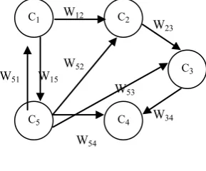
The term cognitive map (CM) appears for the first time in 1948's in article by E. Tolman [6] cognitive maps in rats and men to describe the abstract mental representation of space built by rats trained to navigate in the labyrinth. The term FCM (Fuzzy Cognitive Map) was introduced in 1986 by B. Kosko [2], to describe a simple extension of CMs by the combination of fuzzy logic and artificial neural networks. This robust combination given FCMs a structure similar to artificial recurrent neural networks (Artificial Recurrent Neural Network ARNN. FCMs (Figure 1) can describe the complex behavior of entities. They are represented as directed graphs whose nodes are concepts (classified into three types: sensory, motor and effectors) and the arcs represent causal relationships between these concepts. Each arc from one concept Ci to one concept Cj is associated with a weight wij reflecting a relationship of inhibition (wij <0) or excitation (wij > 0). Each concept is associated with a degree of activation, represent's the state at time t, and can be modified over time. The dynamics of an FCM can be summarized in one cycle (from t to t +1) by updating the activations vector.

Fig 1: An FCM as a graph

The following gives a formal description of an FCM [7]. K denotes one of the rings or , by δ one of the numbers 0 or 1, for V one of the sets {0, 1}, {-1.0, 1}, or [-δ,a]. Let

(n, t0) ∈ IN² and k ∈ *+. An FCM F is a sixfold

(C, A, W, A, fa, R):

• C = {C1, …, Cn} is the set of n concepts forming the nodes

of a graph.

• A ⊂ C × C is the set of arcs (Ci, Cj) oriented from Ci to Cj.

• W: C×C→K

C1 C2

C3

C5 C4

W12

W53

W54 W25

W34 W51

W23

(Ci, Cj) → Wijis a function of C×C to IR associating a weight Wijto a pair of concepts(Ci, Cj), with Wij = 0 if (Ci, Cj) ∉ A, or Wij equal to the weight of the edge if (Ci, Cj) ∈ A. Note that W(C × C) = (Wij) ∈ Kn × nis a matrix of Mn (IR).

• A:C→Vn

Ci→ai is a function that maps each concept Ci to the sequence of its activation degree at the moment t ∈ IN, ai (t) ∈ V is its degree of activation at the moment t. We Note a (t) = [(ai (t)) i ∈ [[1, n]] T the vector of activations at the moment t.

• fa ∈ (IR n) N is a sequence of vectors of forced activations such as for i ∈[1, n] and t ≥ t0 is the forced activation of the concept Ci at the moment t.

• (R) is a recurrence relationship on t ≥ t0 between ai (t +1), ai(t) and fai(t) for i ∈[1,n] indicating the dynamics of the map F.

(R) : ∀i ∈ [1, n], ∀t ≥ t0,

ai (t0) = 0

ai (t+1) = σ[gi(ƒ ai(t),∑j∈[1,n]Wij aj(t))]

ƒ (x) = 1/(1+e-x_{) ƒ (x) = 1 si x ≥k ƒ (x) = 1 si x≥k}

0 si x ≤k 0 si x = k

-1 si x≤k

Fig 2. Cognitive maps’ standardizing function.

The Mode represented by the function  is to reduce the value of concepts within the range of values taken as the area and can be either binary, ternary and sigmoid. The value of each concept is calculated with original formula proposed by Kosko [2]:

_{}_{}

Other alternatives involve taking into account the past history of concepts and jointly proposed the following equation:

_{}__

(2)

The Algorithm 1 shows the steps to follow for the calculation of the next input vector .

2.2.

Reinforcement Learning (RL)

The Markov Decision Processes (MDP) defines the formal framework of reinforcement learning [8]. More formally, an MDP process is defined by:

• S, a finite set of states. s Є S

• A, a finite set of actions in state s. a Є A(s)

• r, a reward function. r(s, a) Є R

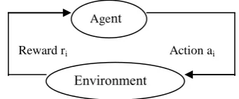
• P, the probability of transition from one state to another depending on the selected action P (s '| s, a) = Pa(s, s'). The problem is to find an optimal policy of actions that achieves the goal by maximizing the rewards, starting from any initial state. At each iteration, the agent being in the state chooses an action, according to these outputs the environment sends either award or a penalty to the agent shown by the following formula: ri = h (si, ai, si+1).

Fig 3 : Agent-environment Interaction in reienforcement learning

To find the total cost, which is represented by the formula Σ h(si,ai ,si+1), the costs are accumulated at each iteration of the system. In [9] the expected reward is weighted by the parameter γ and becomes Σ γ h (si,ai,si+1) with 0 ≤ γ ≤ 1. The RL is to find a policy or an optimal strategy π *, among the different π possible strategies in the selection of the action. Q-Learning algorithm [8] is to introduce a quality function Q represents a value for each state-action pair and Qπ _{(s, a) is to} strengthen estimate when starting from state s, executing action a by following a policy π: Qπ_{(s, a) = E Σγr}

i and Q*(s, a) is the optimal state-action pair by following policy π* if Q*(s, a) = max Qπ_{(s, a) and if we reach the Q*(s}

i, ai) for each pair state-action then we say that the agent can reach the goal starting from any initial state. Initially, the Q values are initialized most cases to 0 and the value of Q is updated by the equation:

Qk+1_(s

i,ai) = Qk (si,ai) + α[h(si,ai ,si+1) + γ arg max(Qk(si+1,a)) - Qn _(s

i,ai)] (2)

α is called learning parameter.

Algorithm 1: Calculation of the output vector

Step 1: Read the input vector _{and weight matrix W.}

Step 2: Calculate the output vector _

_{}_

Step 3: Apply the transfer function  to the output vector 

Step 4: verify the conditions of termination of the algorithm

0 1

-1 0 1

Sigmoid mode _{Binary mode} ternary mode

Agent

Environment

3.

THE ADAPTATION OF LFCM

The CASs [10] are distinguished from other systems by their dynamic improvements in current policy for each interaction with the environment. So this is a local building that does not require an assessment of the overall strategy. This observation leads us to overlook the value of the quality function Q in step (i+1). This translates mathematically by: Qn(si+1, a) = 0 and therefore equation (2) of the function Q becomes as follows:

Q (si, ai) = Q (si,ai) + α [ri - Q (si, ai)] (3) The following pseudo code provides an update of the value of Q function:

If r = 1 / / Award

Q(si, ai) = Q(si,ai) + α[1- Q(si,ai)] If r = 0 / / Penalty

Q(si,ai) = (1 - α) Q(si,ai)

In our approach, if the states are represented after fuzzyfication by the concepts inputs or sensory concepts, the output vector is represented by the set of output concepts or effectors concepts that represent actions to perform in the environment after defuzzyfication. The motors concepts are the decision-making mechanism.

The value of Q is designed to instruct the agent to consider optimally its historical past. If the agent is in a state already visited, with a Q value in the table of values, it will be directly exploited to move to the next state, otherwise it will explore the possible actions in this state according to their respective probabilities. The exploration of the actions is accompanied by an update of their probabilities according to the linear scheme [11]:

If r = 1 / / Award

P (si, ai) = P(si,ai) + β (1 - P(si,ai))

If r = 0 / / Penalty

P(si, ai) = (1-β) P(si,ai)

4.

THE PROPOSED APPROACH

Based on the theoretical aspects described above, the pseudo code of Algorithm 2 summarizes our approach.

Algorithm 2 : Pseudo code of the proposed appoach Step 1: Read the vectork _{and weight matrix W} Step 2: Calculate the output vector k_:

kkk _W

Step 3: Apply the transfer function  to the output vector k_

Step 4: Among the active concepts choose the one that has the highest value of the function Q, if not probability Step 5: calculate the new output vector (output concepts)  _k

Step 6: Depending on the response to the environment: If r = 1 / / Award

(Updating the probability Pij and the Q value) Q (s, a) = Q(s,a) + α [1 – Q(s,a)]

WCi,Cj) = WCi,Cj)

P(ai) = P(ai) + β [1 - P(ai)]

If r = o / / Penalty

(Updating the probability Pij, the weight of the connection and the value of Q)

Qk _(s

i, ai)) = (1- α) Qk (si, ai)

WCi,Cj) = WCi,Cj) +η [1 - WCi,Cj)]

P(ai) = (1-β) P(ai)

Step 7: If the termination conditions are realized Stop. Otherwise go to Step 2

5.

THE PREY AND PREDATOR MODEL

SIMULATION

It is assumed that the prey in a presence of a predator has only two actions to be taken for escape. Leak to the right (LR) and Leak to the left (LL). The use of probabilities of actions and values of the function Q provide a compromise between exploration and exploitation of actions. An FCM to represent this model in the theoretical framework of FCMs can be outlined as follows:

0 0 +1 0 0

0 0 +1 0 0

W = 0 0 0 +1 +1 0 0 0 0 0

0 0 0 0 0

Fig 4 : FCM's escape behavior of prey against its predator and W matrix link

Sensory Concepts-(Inputs Concepts)

+1 +1

Motor Concept

+1 +1

Effectors Concepts-(Outputs Concepts) Fear

PN

LL

PF

LR

C1 C2 C3 C4 C5 C1

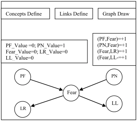
Fig 5: Main view of LFCM tools

Concepts C1, (PF) for the Predator Far, and C2, (PN) Predator Near, are the inputs sensory concepts. The concepts C4 (LR), Leak Right, and C5 (LL), Left Leak, are taken as effectors outputs concepts and concept C3 (Fear) is a concept motor. The FCM (Figure 3) has four edges and five concepts with links excitatory (+1) of 'NP' to 'Fear' and 'Fear' to 'LR' and 'LL', and linked inhibitor (-1) of 'PF' to ' fear'. Activation of sensory concepts NP and PF fuzzyfication is achieved by the distance to the predator, while the defuzzification gives to escape a recession velocity for this agent.

The concept is active if its value is 1, otherwise it is inactive (binary mode). It is given an initial activation vector A = (0 1 0 0 0). Table 1 show’s the values P(ai) of the probabilities of actions and values of the function Q updated at each iteration. Table 2 gives the output vector for all iterations in response to the environment.

Table 1. Action probabilitiesand Q-Function values

ai P(ai) Q(si, ai) value

LL

LR 0.5

0.5

(NP,LL)

(PF,LR) 0

0

Table 2. Output Vector

At iteration n ° 3 the prey is facing a situation where it has two possible actions, represented by the active concepts C4 and C5, but must choose one among them and this choice is guided either by the value of function Q, if the state is already visited, or by the value of the probability of the action if the first pass in this state.

6.

Related work

We have selected two axes to compare our approach with the approaches used by the different teams in the field of intelligent modeling of dynamic systems. The first concerns the graphical representation and the second axis concerns the mathematical description of the studied system.

1. The FCMs graphical representation can view the structure of the studied system in the form of concept (node) that represent a state, a propriety or other characteristic of the modeled system, connected by causal relationships that determine the nature of the action exerted on each other concepts which it is connected. This graphical representation can develop relatively simple and readable models something that is not found in the AMAS theory [12] and in the cellular automata field [13].

2. The FCMs mathematical foundations [4] can express the behavior of the investigated system in algebraic form. The future state of the system is derived by simply applying algebraic methods represented here by the multiplying the current state vector with the causal links matrix and the result of the operation gives a new state vector to be used as an input for the nest step.

7.

ACKNOWLEDGMENTS

The authors would like to thank reviewers and colleagues for their valuable comments and suggestions about originality in modeling field of the intelligent systems.

8.

CONCLUSION

The complexity and criticism raised by the community in the field of modeling CASs by MASs and CAs, led us to seek another approach, which is contained in same concepts inspired by the area of life. In psychology behavior is generally related to the concepts of emotions, perceptions and sensations. These key concepts of life can be supported by FCMs. CASs are therefore in the field of artificial life more than other areas of computing. The area of FCMs, despite the improvement made by different research teams in the world, remains an area dense, low-unified.

9.

REFERENCES

[1] Axelrod Robert (1976). Structure of decision. Princeton university press, Princeton, NewJersy.

[2] Kosko B., Fuzzy Cognitive Maps, International Journal Man-Machine Studies, 24:65-75, 1986.

[3] Maikel León1, Ciro Rodriguez1, María M. García1, Rafael Bello1, and Koen Vanhoof ‘Fuzzy Cognitive Maps For Modeling Complex Systems’. © Springer-Verlag 2010.

[4] Chrysostomos D. Stylios and Peter P.Groumpos. ‘Modeling Complex Systems Using Fuzzy Cognitive Maps. IEEE transactions on systems,Man and cybernetics. January 2004.

Inputs Output vector Iteration

(0 1 0 0 0) 0 1 0 0 0

0 1 1 0 0

0 1 1 1 1

0 1 1 1 0

1

2

3

4 Fear

PN

LL

PF

LR

Concepts Define Links Define Graph Draw

PF_Value =0; PN_Value=1 Fear_Value=0; LR_Value=0 LL_Value=0

[5] Elpiniki Papageorgiou and Peter Groumpos. ‘A Weight Adaptation Method for Fuzzy Cognitive Maps to a Process Control Problem’. Springer 2004.

[6] E. Tolman. Cognitive maps in rats and men. Psychological Review volume 55, 1948.

[7] C. Buche, P. Chevaillier, A. N´ed´elec, M. Parentho¨en and J. Tisseau ‘Fuzzy cognitive maps for the simulation of individual adaptive behaviors’ Wiley Online Library 2010.

[8] E.A. Jasmin. T.P. Imthias Ahamed. V.P. Jagathy Raj. ‘Reinforcement Learning approaches to Economic Dispatch problem’. Elsevier_ 2011.

[9] Richard S. Sutton and Andrew G. Barto. ‘Reinforcement Learning: An Introduction’. A Bradford Book The MIT Press Cambridge, Massachusetts London, England 2005.

[10]Linda Groff, Rima Shaffer. 'Complex Adaptive Systems and Futures Thinking: Theories, Applications, and Methods'. Special Issue Futures Research Quarterly • Summer 2008.

[11]“TSP Home page”, http://comopt.ifi.uni-heidelberg.d/software/TSPLIB/index.html.

[12]Davy Capera, Jean-Pierre George, Marie-Pierre Gleizes, Pierre Glize. 'The AMAS theory for complex problem solving based on self-organizing cooperative agents'. Proceedings of the Twelfth IEEE International Workshop on Enabling Technologies: Infrastructure for Collaborative Enterprises. IEEE 2003.

[13]

Hamid Beigy, Mohammad Reza, Meybodi

'Cellular Learning Automata With Multiple Learning Automata in Each Cell and Its Applications'. IEEE

transaction on systems, man, and cybernetics—Part B: Cybernetics, VOL. 40, NO. 1, Februrary 2010.

[14] Pradipta K Das, S C Mandhata, H S Behera and S N Patro. Article: An Improved Q-learning Algorithm for Path-Planning of a Mobile Robot. International Journal of Computer Applications 51(9):40-46, August 2012. Published by Foundation of Computer Science, New York, USA.

[15]AH Tan, YS Ong, A Tapanuj 'A hybrid agent architecture integrating desire, intention and reinforcement learning'. Expert Systems with Applications, 2011 - Elsevier

[16]H. Van Dyke Parunak A Mathematical Analysis of Collective Cognitive Convergence. AAMAS 2009 • 8th International Conference on Autonomous Agents and Multiagent Systems • 10–15 May, 2009 • Budapest, Hungary.

[17]Matthew E. Taylor , Peter Stone, 'Transfer Learning for Reinforcement Learning Domains: A Survey'. Journal of Machine Learning Research 10 (2009) 1633-1685. [18]Sevan G. Ficici, Avi Pfeffer, 'Modeling how Humans

Reason about Others with Partial Information'. Proc. of 7th Int. Conf. on Autonomous Agents and Multiagent Systems (AAMAS 2008), Padgham, Parkes, Müller and Parsons (eds.), May, 12-16.2008, Estoril, Portugal, pp. 315-322.