LOAD CURRENT CONTROL BASED ON LUENBERGER OBSERVER FOR THREE PHASE POWER CONVERTER SVPWM

COMPREHENSIVE COMPARISONS OF THREE

LOCALIZATION ALGORITHMS USED IN WSN

1

MA XIANGXUE, 2XING JIANPING, 2,3LIU YANG, 3WU HUA

1

School of Mechanical, Electrical & Information Engineering, Shandong University at Weihai

2

School of Information Science and Engineering, Shandong University

3

School of Information Science and Electric Engineering, Shandong Jiaotong University

*Corresponding Author

E-mail: [email protected], [email protected]

ABSTRACT

In this paper, we made comprehensive comparisons of three localization algorithms in wireless sensor network (WSN): A localization algorithm based on virtual central node (VCN), an improved 3D node localization algorithm based on virtual central node (IVCN) and an iterative calculation of secondary grid division (ICSGD) localization scheme. VCN and IVCN algorithms are both adapted to the wireless sensor network (WSN) that anchor nodes present an uniform distribution in three dimensional sensor spaces. During the localization process, by deducing a 3D special node, which is called the virtual central node, unknown nodes can compute their own positions automatically. Iterative calculation of secondary grid division (ICSGD) localization scheme could solve the inconsistency between calculation amount and location accuracy. The performance of the localization scheme was evaluated in a series of simulations performed using MATLAB. The simulation results demonstrated that the three schemes outperform in terms of higher location accuracy, and lower location amount.

Keywords: WSN, Localization Algorithms, ICSGD, VCN, IVCN

1. INTRODUCTION

Wireless sensor networks (WSNs) consist of sensor nodes capable of collecting environmental information from surrounding and communicating with each other via wireless transceivers. Typical sensor networks consist of a large number of densely deployed sensor nodes. Until now there has been an increase in the use of ad hoc wireless

sensor networks (WSNs) for monitoring

environmental information, such as intrusion detection, traffic management, space exploration, water quality monitoring, precision agriculture design and disaster rescue. Emerging applications will depend on automatic and accurate location of thousands of sensors. If the positions of sensor nodes can be located more accurately, the data transmission of the network will be more efficient.

Until now, WSN localization scheme has been widely researched, a large amount of which can be found in [1] and [2], but there is yet much work to do in the field. One typical way is to use global positioning system (GPS) to realize locating. However, each sensor node is limited on power

consumption and other costs. So GPS is not a feasible way for WSN node.

Some special localization algorithms for WSN have been proposed [3]. The general localization mechanisms proposed before can be mainly classified into range-based approaches and range free approaches. The former approaches determine the node position fully based on distance or angular information acquired using the Time of Arrival (TOA), Angle of Arrival (AOA), Time Difference of Arrival (TDOA), or Received Signal Strength Indicator (RSSI) techniques [4]. Rage-based algorithms have higher localization accuracy but require extra hardware on nodes to make them capable of measuring distances, which would inevitably require more construction costs and power consumption. Also, these measurements can be vulnerable to environmental issues, such as noise, temperature and humidity [5].

improved obviously and operates more stable than before and is robust to environments.

We have done a lot of work in node localization algorithm in WSN. The three algorithms, ICSGD, VCN and IVCN, are all proposed by our work. And simulation results prove that they have better performances.

The remaining paper is organized as follows: Section 2 describes ICSGD, VCN and IVCN algorithms in detail. Explicit algorithm realizing processes are presented. And performance simulations are made in MATLAB software and simulation results are given in Section 3. We make some conclusions in Section 4.

2. REALIZATION OF THE ALGORITHMS

In this scheme, nodes were divided into two categories: beacon node and unknown node. Beacon nodes could get their accurate position information with the help of GPS receivers, while unknown nodes had to calculate their position according to the position of beacon nodes. The beacon nodes could locate themselves accurately by GPS receivers, and they could control transmitting power. The system environment included a number of beacon nodes and unknown nodes. All nodes are randomly deployed in a three-dimensional cube. The localization scheme required some fundamental assumptions as follows.

All nodes were static. Once nodes were randomly deployed, the position of each node was fixed. Each beacon node was equipped with a GPS receiver or some other forms of localization device to get accurate position information. The signal was transmitted in an ideal model, and there was no loss during transmission process. Each node was equipped with omni-directional antenna, which could receive the signal of all directions.

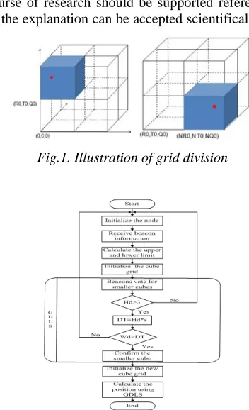
When an unknown node received the information of beacon nodes, it stored the information into its local information table, which was shown in Table 2. The table included sensor ID, beacon ID and beacon coordinates. After calculation, it also stored the upper limit of layer 1 and layer 2, lower limit of layer 1 and layer 2, first locating coordinates and second locating coordinates into its table which is shown in Figure 1.

Explain the research chronological, which includes research design, research procedure (in the form of algorithms, Pseudocode or other), how to test and data acquisition [3]. The description of the

course of research should be supported references, so the explanation can be accepted scientifically [6].

Fig.1. Illustration of grid division

Fig. 2. Flow of an unknown node localization

Each beacon node broadcast its beacon information in the whole network. At first, it increased its power level according to layer 1, after certain time, it increased power according to layer 2. When an unknown node received its beacon information, stored the information into local information table, and calculated the upper and lower limit of layer1 and layer2, which was shown in Fig.2. With the help of upper and lower limit of layer 1, it could calculate the first coordinates using GDLS. Then, it could calculate the second coordinates according to the upper and lower limit of layer 2 and the first coordinates using GDLS again.

In our proposed algorithm, all anchor nodes are supposed to present an uniform distribution in the special 3D sensing space. In this algorithm each sensor node estimates its position solely based on the information gathered directly from the anchor nodes. Since it does not depend on neighboring sensor node communication, it is independent of network connectivity and it is more suitable for all kinds of complicated applications.

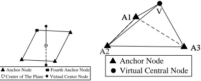
can be set manually. The data information includes anchor node ID, and coordinates of corresponding anchor nodes. Unknown nodes’ task is easy and energy efficient because they are only in charge of listening to these packages in the time slice T. Unknown nodes can memory how many packages have received from different anchors. Then they judge whether the time slice T is arrived. If so, the information can be recorded, or go on waiting. As we said in the last part, once the package enters the communication range unknown nodes can detect it immediately and record the information data contained in the corresponding packages. At last by the information provided in these packages, virtual central node is formed and can be computed. Finally unknown position can be derived using the virtual sensor node above. By using the center of the square, virtual central node can be computed through adding half of communication range on one of three ordinate directions. But there is a problem in this algorithm. As shown in Fig.3, after the fourth node is determined, we cannot make sure the virtual central node is on which side of the plane. It may be on the same side with unknown node which means low estimation error. However, if it is on the opposite side of the unknown node, it will produce a lot of localization error. During our localization algorithm, the position of virtual central node on which side is decided randomly and of course it is not a perfect solution which can induce lots of uncertainty. Of course how to solve this problem completely is also a research direction in the future to make higher and better localization accuracy.

Anchor Node Fourth Anchor Node Center of The Plane Virtual Center Node

A1

A3 V

A1

A3 A2

Anchor Node Virtual Central Node

Fig.3 Derivation of unknown node position

When the virtual central node is found out, unknown nodes can finish the localization process. As shown in Fig.2, three anchor nodes (A1, A2, and A3) and virtual central node V form a tetrahedron. Of course this tetrahedron is anomalous. The virtual central node could be either side of the plane determined by node A1, A2, and A3. Then we can use the similar way of Centroid algorithm. That is to say the center of the four special nodes is the estimated position of the unknown node. It is necessary to illustrate the feasibility of this method. As we know, virtual central node is important in

this algorithm. Based on this unknown node the center of a 3D graph could be computed.

The centroid of the four nodes (three anchors and virtual central node) with determined position is used as the estimated coordinates of unknown nodes.

3. SIMULATION RESULTS

In this section, we are going to study the performance of ICSGD and IVCN in MATLAB software.

Figure 4 showed the average location error of

GDLS and ICSGDLS in a cube of

500

m

it, it could be seen that the average location error decreased as the radio power range of beacon increased. The average location error of GDLS decreased from 0.4308R to 0.2146R as beacon power range increased from 200m to 400m. However, the average location error of ICSGDLS (25+5) decreased from 0.3573R to 0.0692R, and the average location error of ICSGDLS (10+10) decreased from 0.6480R to 0.1306R. Although the cycles of an unknown node in ICSGDLS (25+5) increase by 0.19%, the average location error decreases by 67.7%. The performance of ICSGDLS (10+10) was also better than that of GDLS at a much lower cost when the power range of beacon reached 400m. As shown in Figure 4, the average location error of GDLS could reach 0.2103R in a

cube of ₂₀3_m3 _{when the power range of beacon}

node was 16m. However, the average location error of ICSGDLS (25+5) could be reduced to 0.0808R.The average location error decreased by 61.6%.

Fig.4. Average location error of GDLS and ICSGDLS in a cube of

500

m

margin. In the second division, only the selected cube was divided. As a result, a higher accuracy could be acquired. Through this, the relationship between accuracy and amount of calculation could be dealt with very well. Simulation had shown the scheme had high accuracy, and the average location error of unknown nodes could reach 0.35m in a

cube of

500

m

communication between unknown nodes, communication spending could be reduced. Therefore, unknown nodes could make full use of energy they took. The localization of an unknown node was finished by itself, and didn’t rely on other unknown nodes. When some unknown nodes were damaged, the other nodes could still be located. Therefore, the scheme was robust.

In this part, comparisons of IVCN algorithm with classic two dimensional DV-Hop and Centroid are given.

Fig.5 Error comparisons of IVCN, VCN, DV-Hop and Centroid under different communications

We vary the number of deployed unknown sensors to get different node density and connectivity with R=15m, 20m, 25m, 30m, 35m, and 40m respectively. Here percentages of anchor nodes are altered from 5% to 50% and estimation error is recorded in each situation with other network settings the same. The six sub-graphs in Fig.6 describe the estimation error under different percentages of anchors of IVCN, VCN, DV-Hop, and Centroid with varied communication range R. All the four localization algorithms take advantage

of the distance estimation to anchors for estimating sensors’ positions in WSNs. There is no doubt that more accurate distance measurement leads to better position estimation. The four curves preserve approximate straight line. DV-Hop algorithm is the worst of the four no matter how the environmental parameters change. Its estimation error always stays at a high level. Centroid algorithm performs the best when communication range is no larger than 35m. From Fig.4, we can conclude that communication range is the main factor of IVCN, VCN, and Centroid which affect the localization accuracy.

Fig.6 Error comparisons of IVCN, VCN, and other two with different communication ranges. Once communication range R is set as 35m or larger than that, IVCN and VCN outperform Centroid become the best of all. IVCN is little better than VCN on the localization error especially R is set as 40m. This is due to the fact that the lager the communication range, the more information packages could be able to be received by unknown nodes, the more accurate the position estimation will be. IVCN constrain the possible position of unknown nodes into a smaller space which increases the localization accuracy of the whole algorithm.

error always stays at a high level. Centroid algorithm performs the best when communication range is no larger than 35m. From Fig.4 we can conclude that communication range is the main factor of IVCN, VCN, and Centroid which affect the localization accuracy.

4. CONCLUSIONS

In ICSGDLS scheme, forty beacon nodes and five hundred unknown sensor nodes were randomly deployed in a cube, which is divided into smaller cubes twice. The position information of unknown nodes could be got by iteratively calculating the centroid of smaller cubes. However, in IVCN algorithm, localization problem is solved by deducing a 3D special node that is called virtual central node (VCN) from three different anchor nodes and the deducing process is more simplified. The unknown position coordinates can be obtained by the whole four node position information finally. The simulation results prove the performance of our IVCN. Meanwhile, as computing coordinates once 3 distances are received, IVCN decreases the overload of the whole network. In the simulation graphs provided in Section 3, IVCN overcomes the defects of VCN. Also it retains the advantages of VCN. IVCN is not only the improvement of VCN but also extends the application fields of the algorithm. So it is suitable for the situation needs quick localization. Based on these properties we are thinking how to use it in mobile node localization using IVCN in mobile wireless sensor network environment. Through analysis we can find that VCN and IVCN algorithms are both two high efficient which used in 3D wireless sensor networks. They can both realize localization with high accuracy. But to some extent IVCN is better than VCN.

We found these algorithms cannot be suitable in mobile environment. If we use in mobile nodes, low localization accuracy can be proved. So we will do some research in mobile environment in the future.

REFRENCES:

[1] G. Mao, B. Fidan, and B. D. O. Anderson,

“Wireless sensor network localization techniques,” Computer Networks, vol. 51, pp. 2529-2553, 2007.

[2] S. Gezici, “A survey on wireless position

estimation,” Wireless Personal Communications, vol. 44, pp. 263-282, 2008.

[3] A. Savvides, H. Park, and M. Srivastava, “The

bits and flops of the N-hop multilateration primitive for node localization problems,” Proc. WSNA’02, Atlanta, USA, pp. 112-121, Sept. 2002.

[4] K. F. Ssu, C. H., Ou. and H.C. Jiau,

“Localization with mobile anchor points in wireless sensor networks,” IEEE Trans. Veh. Technol., vol. 54, no. 3, pp.1187-1197, 2005.

[5] T. S. Rappaport, J. H. Reed and B. D. Woerner,

“Position Location Using Wireless Communications on Highways of the Future,” IEEE Comm. Magazine, vol. 34, no. 10, pp. 33-42, Oct. 1996.

[6] J. Aspnes, T. Eren, D. Goldenberg, A.S. Morse,