Electrocavitation in nanochannels

Full text

(1)MASTER THESIS. ELECTROCAVITATION IN NANOCHANNELS. D.S. van Schoot. ELECTRICAL ENGINEERING BIOS EXAMINATION COMMITTEE. Prof. Dr. J.C.T. Eijkel Dr. Ir. N. Tas Dr. Ir. P. Vulto Prof. Dr. Ir. A. van den Berg. DOCUMENT NUMBER. BIOS - 2012-13. 5 OCTOBER 2012.

(2)

(3) Abstract Cavitation in water has been the subject of research for centuries. This thesis investigates a novel method for cavitation that was dubbed electrocavitation. It employs concepts of nanofluidics to create a platform to study cavitation that can be easily controlled and where cavitation can be reliably generated. It works by applying a voltage axially over a nanochannel where a conductivity step is present in the solution. This generates a tension in the solution which, at sufficiently low pressures, causes it to cavitate. The advantages of this setup over traditional methods of cavitation are that it is less cumbersome, more reliable and predictable and able to reach very high negative pressures. This thesis focusses both on the technical aspects of this method as well as the theoretical framework to interpret the cavitation experiments. First of all, an already existing setup is enhanced and upgraded to include electrical current measurements in the determination of cavitation experiment characteristics. These are the immediately employed in measurements. A theoretical framework is also provided to understand all the measurement results and make predictions about the measurements, including a part about the fundamentals of cavitation in general. With the help of the electrical current data a new set of measurements could be performed. One of the most important ones is a determination of the ζ-potential, an important quantity in nanofluidics in general and in electrocavitation in particular. This in turn is used to calculate the pressure everywhere in the channel during the electrocavitation experiment. It could then be proved that the position of cavitation coincides with the position of the front between the two solutions used for cavitation. The cavitation location moves over time and eventually disappears, suggesting the pressure at that moment is not low enough to make the solution cavitate. It is concluded that a reliable platform has been developed for cavitation experiments. It has potential to reach very low pressures and thereby tell new things about the behaviour of salty aqueous solutions. It can be further used to investigate for example the structure of water in salty solutions with use of the Hofmeister series.. iii.

(4)

(5) Preface This thesis marks the end of my studies in Electrical Engineering at the University of Twente. This has been an important and pleasant period of my life, in which I not only learned how to be an engineer, but also developed myself more broadly and built some very fond memories. I was never fascinated with die-hard electronics and engineering. Instead, at almost every instance I learned and discovered something new I asked myself: What is the bigger use of this? How does this benefit people or society? But also: How does this really work? Which forces are at play here? These questions motivated me to try to get the most out of every course I attended. However, even motivation is not always enough. Without the support of friends, family and teachers, it is hard to keep on the right track. In this preface, I would therefore like to thank everyone that supported me during my time at the university. First of all, I would like to thank professor Jan Eijkel for his endless enthusiasm and optimism, his active support for my personal plans and offering this research opportunity to me in which I got to sample a different living environment in the last stage of my engineering studies. I am thankful that I got to work with Kjeld, who has a lot of energy and was always ready to answer my questions and discuss with me in his own time. I think working on this more conceptual project would have been very hard if Niels had not been there. The discussions we had made me realise what things are really important, both in science and in life. I would like to thank Albert too for his interest in this research and making it all possible. I am very grateful to Paul at the Analytical Biosciences group in Leiden. He quickly introduced me to the group and made my last few months of studying a very pleasant time, inviting me to a congress in my first two weeks there. Discussions with him were always no-nonsense and to-thepoint yet at the same time very open, which I found quite refreshing and always gave me new energy afterwards. I enjoyed being surrounded by fellow students at both Leiden University and the BIOS-group. This applies especially to Marco, who somehow always managed to say the right things when I needed that little bit of extra motivation. Someone who helped me out many times on the technical side is Raphaël. The times I visited him when something trivial or nontrivial broke down are countless, though he was always happy to see me and tried to help me as soon as he could. I would have never found the energy to undertake this project without the encouragement of my friends. They were always frank in their interest for my endeavours and helped me with some of the problems I encountered. My parents gave me good support as well, and they made all of this possible in the first place. I want to thank them for that. Special thanks go to Fiona. I would like to thank you for believing in me and supporting me every day throughout my project. You really motivate me to get the best out of myself and follow my passions. I had a great time, and I will certainly miss the research environment where one is free to investigate if fundamental ideas and concepts will work. Daniël van Schoot, 5 October 2012 v.

(6)

(7) Contents Chapter 1: Introduction ........................................................................................................................... 1 1.1. Cavitation in water: an overview...................................................................................... 1. 1.2. Electrocavitation in nanochannels ................................................................................... 3. 1.3. Problem definition and research outline ......................................................................... 4. 1.4. Thesis outline.................................................................................................................... 5. Chapter 2: Electrocavitaton: bottom-up ................................................................................................. 7 2.1. Manipulation of fluid by a pressure difference ................................................................ 7. 2.2. Flow caused by electrokinetic effects .............................................................................. 8. 2.3. A channel with a conductivity step, a rough approach .................................................. 11. 2.4. A channel with a conductivity step, a more exact approach ........................................ 12. 2.5. The electrical current and its properties ........................................................................ 15. 2.6. Putting everything together: electrocavitation .............................................................. 16. Chapter 3: Methodology ....................................................................................................................... 19 3.1. The nanochannels and their fabrication ........................................................................ 19. 3.2. The setup to perform electrocavitation ......................................................................... 20. 3.3. The used solutions and their preparation ...................................................................... 23. 3.4. Measurements performed using the setup ................................................................... 24. Chapter 4: Experimental results ............................................................................................................ 27 4.1. Current measurements before and after improvements .............................................. 27. 4.2. EOF measurements to determine the ζ-potential.......................................................... 28. 4.3. Electrocavitation experiments ....................................................................................... 30. 4.4. Hofmeister series experiments ...................................................................................... 37. Chapter 5: Conclusions .......................................................................................................................... 39 5.1. Research aim and findings.............................................................................................. 39. 5.2. Limitations and discussion.............................................................................................. 40. 5.3. Contribution of this thesis .............................................................................................. 40. 5.4. Recommendations for future research .......................................................................... 41. References ............................................................................................................................................. 43 Appendix A: Preparation protocol......................................................................................................... 45. vii.

(8)

(9) Chapter 1: Introduction 1.1. Cavitation in water: an overview. Any liquid can be turned into a vapour by stretching it. By pulling the liquid, it will stretch out and its inner pressure will lower. Eventually, it will return to its equilibrium state by the nucleation of vapour bubbles. This phenomenon is called cavitation. Cavitation in water occurs at many places in nature such as in trees, disrupting their liquid column and stopping the ascending flow of sap (this is called xylem emboly [1]). The sound that can be heard when we crack the joints in our hand is caused by cavitation. The fluid between two joints stretches up to a point where it cannot stretch further. A bubble arises and bursts, producing the characteristic sound [2]. An application of cavitation can be found in ink jet printers where it is used to produce microbubbles which are in turn used to eject a drop of ink out of a nozzle. Cavitation in water can also cause damage to the propeller blades of ships [3]. Besides having all these effects, cavitation gives us information about the fundamental behaviour of water, namely its thermodynamic properties and limits. The main reason why liquids under tension (negative pressure) are interesting to study is that their behaviour is dominated by intermolecular attractive forces rather than by short-range repulsive (steric) forces [4]. Particularly for water this gives information about the hydrogen bond network between different water molecules. Predictably, there has already been much attention given to the case of water. The first experimental observation of negative pressure was made in 1662 by Christiaan Huygens, using the weight of water itself to generate the pull [5]. His experiment was presented to Royal Society of England and repeated on water and mercury by physicists Hooke and Boyle [3]. Reynolds reached a negative pressure of -0.3 MPa (or -3 bar) using this technique. Research into actual cavitation of water has been carried out since the 1840s using the Berthelot method, named after its inventor Marcellin Berthelot [6]: a vessel is filled with a liquid, sealed and then heated up. It is then cooled down again and the liquid will stick to the wall while the pressure decreases. For low enough temperatures, the pressure will be negative and the liquid will cavitate [3]. Depending on the material of the vessel, pressures of -16 MPa [7] and -18.5 MPa [8] can be reached. There are two types of nucleation and thereby cavitation: homogeneous and heterogeneous. Homogeneous cavitation takes place in a bulk liquid and the transition to vapour takes place due to thermal fluctuations of the system. Heterogeneous cavitation is usually triggered by impurities or walls that function as nucleation sites. In a liquid that is under tension, nucleation of the liquid into its vapour phase is energetically favourable, since a bubble will experience a pulling force. However, this nucleation process is hampered by the energy cost of forming a liquid-vapour interface. The balance between these energies results in an effective energy barrier which has to be overcome for the bubble to grow spontaneously. Theory predicts a minimum pressure that can be attained before the water will inevitably cavitates, depending on the temperature and the used volume and reaction time. At room temperature this ranges from about -140 MPa to -200 MPa [9].. 1.

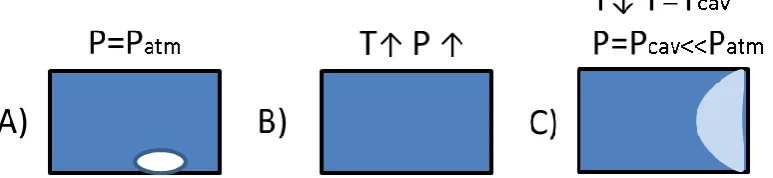
(10) 2. Chapter 1: Introduction. Albeit the minimum pressure before cavitation can be very low, most techniques produce disappointing results in the range of -20 MPa to -30 MPa. They include the aforementioned Berthelot method as well as a method called centrifugation, first used by Reynolds around 1880 [10]. In the method, water is rotated in a tube at high speed. A negative pressure arises because of the centrifugal force. The lowest pressure obtained using this method is -27.7 MPa [11]. Another method involves creating shock waves using fibers and lasers. The maximum negative pressure there is claimed at -27 MPa [12]. Acoustic cavitation is a different technique where a high amplitude sound wave is focused in the bulk liquid. Negative pressures arrive during the negative swing of the acoustic wave. Pressures down to -24 MPa have been achieved using this technique [9]. None of these methods comes close to theoretical limits. However, one method, first performed in 1991, obtains pressures down to -140 MPa [4, 13]. The principle is the same as in the Berthelot method. Water trapped in small inclusions in quartz crystals can be found in nature or synthetically produced. The water is then heated until there are no more bubbles and is subsequently cooled down until it cavitates. A reason why this method works better than the others is that water adhesion on quartz walls is stronger than in the other methods, leading to a higher tension (lower pressure) before the water cavitates [4]. More recently, the experiment has been repeated with synthetically created inclusions with water and different salts dissolved in the water. The lowest pressure recorded here is -146 MPa using CaCl2 dissolved in water [14]. A schematic overview of cavitation using this technique and the Berthelot method is shown in Figure 1.1. A criticism to the inclusion techniques is that they use a so-called equation of state extrapolation to derive the pressure which may not be entirely in correspondence with the real pressure present since this equation is derived for positive pressures only [9].. Figure 1.1: Schematic overview of cavitation of water (dark blue) using thermal fluctuations (Berthelot method and quartz inclusions method). The closed vessel or inclusion may contain a bubble (A). Subsequently, the temperature is risen until the bubble disappears because of rising pressure (B). Next, the temperature is brought down upon which the liquid gets stressed and experiences tension until the pressure gets so low that the liquid cavitates (C) and goes partly into its vapour phase (light blue in (C)).. A common disadvantage of all methods is that they are rather cumbersome and involve big and expensive equipment. The methods are also rather unreliable and unpredictable as they rely on hard to control thermal methods and fluctuations. Since there is much interest in cavitation and its origins from the field of the physics of fluids, it would be good if there were a platform for cavitation studies and negative pressures that can be easily controlled and where cavitation can be reliably generated. Such a method has recently been discovered. It uses principles of nanofluidics and was christened electrocavitation. An overview of all techniques, their pressure limits and main characteristics is given in Table 1.1..

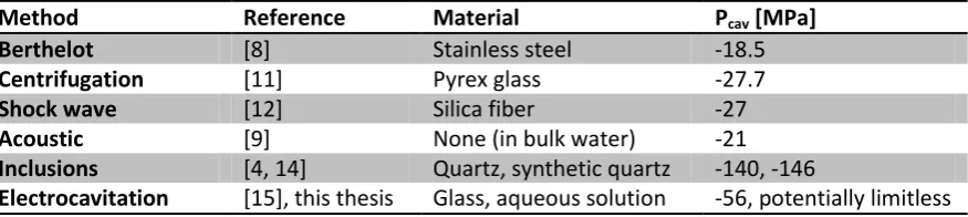
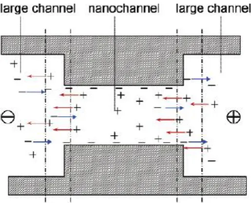
(11) 1.2: Electrocavitation in nanochannels. 3. Table 1.1: A comparison between different cavitation methods. Only the most negative values for each method have been selected. The mentioned material is that of the container, vessel or inclusion the water is in.. Method Berthelot Centrifugation Shock wave Acoustic Inclusions Electrocavitation. 1.2. Reference [8] [11] [12] [9] [4, 14] [15], this thesis. Material Stainless steel Pyrex glass Silica fiber None (in bulk water) Quartz, synthetic quartz Glass, aqueous solution. Pcav [MPa] -18.5 -27.7 -27 -21 -140, -146 -56, potentially limitless. Electrocavitation in nanochannels. A wholly different way from the above to generate cavitation is to apply electric fields over a nanochannel filled with a liquid that contains a conductivity gradient [15]. The conductivity gradient consists of two adjacent fluids with a relatively high conductivity difference. When an electrical field is applied in the lateral direction of the channel, the larger part of it will be over the lower conductivity fluid. This generates a stronger electroosmotic flow (EOF) in this part of the channel. To compensate for this EOF and retain mass conservation, a pressure gradient arises causing liquid to flow against the direction of the EOF in the low-conductivity liquid and along with it in the high-conductivity liquid. This is shown schematically in Figure 1.2. Using an approximation, the negative pressure was calculated to be about -52 MPa (-520 bar) when 500V is applied, with potential pressures theoretically limitless. This new experimental method was dubbed ‘electrocavitation’ when it was first seen in 2011 [15]. This thesis will be about the exploitation and technical refinement of this technique.. Figure 1.2: Schematic overview of electrocavitation. A nanochannel contains two adjacent fluids with a conductivity step and a sharp front. By applying an electric field over the channel an EOF arises from positive to negative potential (indicated by the arrows). The larger proportion of the field will fall over the low conductivity fluid, thus leading to a larger EOF there. The volume flow across the channel however has to be equal (because of mass conservation), this causes a pressure gradient as indicated at the bottom, with the minimum pressure at the front between the two liquids. This in turn generates pressure-driven flow against the EOF on the right and with the EOF on the left [15]..

(12) 4. Chapter 1: Introduction. Zeta-potential gradients leading to pressure gradients had been witnessed and discussed before in microchannels by Herr et al. (in 2000 [16]). They were however more interested in the effect on the efficiency of stacking (that is raising concentrations of samples) and more generally capillary electrophoresis (CE). Fu et al. also considered systems with zeta-potential gradients and looked more explicitly into the pressure gradient. They found the minimum where the zetapotential makes a step. This phenomenon is comparable to the effect of the conductivity step in the liquid i.e. the front between the two liquids [17]. They also found this effect is amplified when the electrical double layers overlap, though this is unlikely in a microchannel. Their main concern is the impact on the efficiency of CE rather than the effect itself. The group of Santiago explicitly considered microchannel pressure gradients generated by conductivity gradients in 2007 [18]. In this case pressures are also limited by the microchannel environment. When using electrocavitation, where the channels are miniaturized further to the nanoscale, the pressure gradient is enhanced since the pressure depends inversely on the height of the channel squared. Moreover, cavitation is observed under these circumstances, emptying the channel. The channel is refilled by capillary action when the electric field is turned off [15]. Since the electrocavitation technique involves preparing water with salts to make solutions of different conductivity, this technique is different from the other cavitation methods where an as pure as possible water sample is used [3]. The cavitation could still be homogeneous but since most of the channel is at strongly negative pressures, breakup may not necessarily occur at the point of lowest pressure. Heterogeneities at the surface (impurities) can also change the position of cavitation and the critical pressure required, similar to what can happen in the Berthelot method. Because the method is based on a nanofluidic electrokinetic principle, it offers more options in terms of variation of experimental parameters such as the height of the channel, the conductivity of the fluids and the applied field. Additionally, as will be shown in this thesis, this method offers great flexibility and reliability in generating cavitation. Furthermore, as different salts can be used, their influence on the intermolecular bonds between water molecules (hydrogen bonds) can be measured. This offers great potential for this setup as a means to study the behaviour of water in aqueous solutions more extensively. Finally it tells us something about the fundamental limits in nanofluidics such as the fundamental limit on the applicable field strength in systems with conductivity gradients. This is relevant to any technique involving conductivity gradients such as isotachophoresis, electroextraction and field-amplified sample stacking, which are all amply used in lab on a chip environments [15].. 1.3. Problem definition and research outline. The research carried out in this thesis project will be on electrocavitation of water in nanofluidic channels. The setup for this research is located at Leiden University at the Department of Analytical Biosciences and was created and maintained by K. Janssen [15]. This project will build on existing results and methods to further study these phenomena and generate further results. The aim is to develop knowledge about this fundamental behaviour of water and its structure. There are four main targets to achieve during this research. Currently, the setup can detect the occurrence of electrocavitation optically, giving information on its movement and location in the channel. From this, the local negative pressure in the channel can be derived. The electrical current through the channel could in addition also provide extremely valuable information on the location of the high/low-conductivity front and the.

(13) 1.4: Thesis outline. 5. magnitude of the electroosmotic flow. However, at the moment the current measurement contains too much noise and is thereby unreliable. The first goal is to go through the whole setup to find the sources of the noise and instability and to eliminate them. Reproduction and confirmation of previous measurements will be tried in order to enhance the reliability of the results with newly available data from the electrical current measurements. The results can also be used to confirm the underlying theory about the involved physics. Additions to the model can also be made, including the effect of diffusion of the interface and concentration polarization at the ends of the channel, among others. While the importance of a sound underlying theory is acknowledged, this thesis does not intend to substantially enhance the existing theory. At this moment the maximum voltage used is 1000V. Theory predicts that the negative pressure will be higher when a higher voltage is applied (in a linear relationship) over the same channel. In results obtained previously by Janssen, a sequence of experiments finds increasingly lower cavitation pressures, and finally no cavitation can be observed at the highest applied potential. The third target therefore is to apply higher voltages and find the corresponding lowest cavitation pressure. The found negative pressure will represent the measured threshold of this method, and can then be compared to other methods. Another aspect is the theoretical explanation of the observed results. This will involve describing the type of nucleation that occurs, i.e. homogeneous or heterogeneous, why it occurs and why the pressure gets lower after each consecutive experiment. Finally, the salts used in the experiments can be replaced by different ones. The aim is to measure how different salts will influence the observed cavitation pressure. By using salts that disrupt the bonding behaviour of water (chaotropes) or enhance it (kosmotropes), the knowledge in the field of cavitation and water structure can be expanded.. 1.4. Thesis outline. Chapter 2 addresses the general theory of nanofluidics and more specifically its electrical aspects. This will then be applied to electrocavitation to describe its characteristics and possibilities. Chapter 3 starts with an elaborate analysis of the measurement setup. Enhancements made to the setup will be motivated as well as various measurement protocols that have been used. Chapter 4 targets the results of all the measurement, the performance of the setup and makes a comparison to conventional methods. Finally, conclusions are drawn and recommendations are given for future work in chapter 5..

(14) 6. Chapter 1: Introduction.

(15) Chapter 2: Electrocavitaton: bottom-up In the remainder of this report the terminology and knowledge of nanofluidics and its applications will be used to describe and interpret electrocavitation. The goal of this chapter is therefore to give an overview of the relevant scientific theory and building blocks in order to come up with a system that can be used to perform electrocavitation.. 2.1. Manipulation of fluid by a pressure difference. Fluidic channels fabricated using microtechnology are called microchannels when their dimensions are in the micrometer range. They are generally called nanochannels when one of their dimensions is smaller than 100 nanometer. Usually these channels are rectangular, i.e. a relatively small height and width and long length. The materials used are usually optically transparent, such as glass or PDMS, a plastic polymer. Nanochannels and their theory will function as the main ingredients to assembly a platform for electrocavitation. One to way to fill a channel with a liquid is by capillary action. This happens when a liquid is introduced at one of the channel ends. Because of surface properties (it can for example be hydrophilic) the channel starts to fill with the liquid. This can be compared to when a small straw is put in a beaker of water; the liquid starts to crawl up the straw, though not very far since gravity holds it down. The velocity in meter per second at which the channel fills is given by Washburn’s equation (for a rectangular channel with height h): ( ). √. Various properties of the channel and the liquid come back in this equation: h is the height of the channel in meters, which is assumed much smaller than the width of the channel (this is generally true for nanochannels), γlg is the surface tension of the liquid/gas (air) interface in Newton per meter, Θ is the contact angle, which is the angle the tangent to the surface makes with the solid surface, η is the viscosity (for water this is 1.001mPa⋅ s at T=300K) and t the time in seconds. An important aspect is that the filling speed decreases with the square root of time. This property can be used to check whether channels have been fabricated correctly by observing them with a microscope while letting them fill up with capillary action. Once the channel is filled, there are several ways the liquid can be manipulated and a flow can be induced. The two most important ways are by applying a pressure, resulting in pressure driven flow (PDF), or by using elektrokinetics, producing an electroosmotic flow (EOF). Both can be derived from solving the Navier-Stokes equations with specific conditions. Applying a pressure difference over the channel can generate a PDF. The resulting flow has a parabolic profile and is also called Poiseuille flow. The average flow velocity in meters per second in the rectangular channel with the width much greater than the height is given by the following equation:. 7.

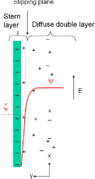
(16) 8. Chapter 2: Electrocavitaton: bottom-up. The pressure applied over the channel is ΔP (in Pascal) and L depicts the length of the channel (in meters). Since the magnitude of the velocity depends on the height of the channel squared and only linearly on the applied pressure, PDF in a nanochannel will be much lower than in a microchannel, with comparable applied pressures. Atmospheric pressure (from the environment) does not influence flow in the channel since it is the same at both channel ends. However, the equation can work both ways meaning that when a flow is present (for example an EOF in a closed channel), it results in a pressure gradient within the channel. This does usually not apply to open channels.. 2.2. Flow caused by electrokinetic effects. When a liquid is present in the form of a saline aqueous solution, it contains cations and anions that spread themselves homogeneously through the solution since any excess of either one will attract the other. However, wall materials such as glass (also known as silica, SiO2) are generally negatively charged because of dissociation of surface groups. In the case of glass walls surface SiOH groups will dissociate protons, creating negatively charged SiO groups. This negative surface charge means that counterions (in this case cations) in the liquid will be attracted to the walls, causing a local excess there. The first layer of counterions is usually held immobile at the surface: this layer is called the Stern layer. This monolayer is not enough to totally screen the negative surface charge so another, thicker, layer of counterions is formed. The ions in this layer are still attracted to the surface though less strongly than the immobile ions, making them able to diffuse away. This layer is called the diffuse layer. Together with the Stern layer they screen the surface charge and are called the (electric) double layer. The bulk of the solution has no excess charge and the potential is generally taken as zero Volts. The walls have a negative charge, so are at negative potential. Through the double layer the potential increases from negative to zero in the bulk. When an electrical field is applied parallel to the surface, all excess ions will feel a body force though only the ones in the diffuse layer can move. The liquid then starts moving along the so-called slipping plane between the Stern and diffuse layer. The potential at the slipping plane is called the zeta(ζ)-potential. All of this is shown schematically in Figure 2.1. Once the liquid in the double layer moves as a result of the exerted body force (by the applied electrical field), it drags the rest of the liquid along by viscous coupling. Viscous coupling means that moving layers of liquid exert a force on the neighbouring non-moving layers until these other layers are all moving with the same velocity. This results in a plug-shaped flow profile. Figure 2.2 gives a representation of what happens. The velocity of the EOF is proportional to the applied field (in Volt per meter) and the electroosmotic mobility, μEOF, which in turn is proportional to the ζ-potential, permittivity and inversely proportional to the viscosity:. This equation is also known as the Helmholtz-Smoluchowski equation. The permittivity (ϵ =ϵr ⋅ ϵ0, relative permittivity (79.1) times permittivity in vacuum, 8.85⋅10-12 Farrads per meter) and viscosity of the solution are more or less constant for aqueous solutions at 7.0⋅ 1010 Farads per meter and 1.001 mPa⋅ s, respectively at a temperature of 300 Kelvin. The applied voltage,.

(17) 2.2: Flow caused by electrokinetic effects. 9. however, can be altered (with ease). This is also possible for the ζ-potential, which depends on the ionic strength of the solution used and the surface potential.. Figure 2.1: The double layer. A negative wall charge leads to excess (positive) counterions close to the wall. These will form a monolayer along the wall (the Stern layer) and a more diffuse layer behind that (diffuse layer). Together they form the double layer. The plane between the Stern and diffuse layer is called the slipping plane and the negative potential there is referred to as the zeta(ζ)-potential. When an electrical field is applied parallel to the wall, the mobile excess ions in the diffuse layer start to move (here against the field). As cited from [19].. Figure 2.2: As a result of the body force exerted by the axial applied electrical field, the excess ions in the double layer start to move. Viscous coupling then drags the rest of the liquid along, resulting in an EOF. The flow profile is the same as the potential profile and thereby plug shaped (except in the double layer). The liquid moves from positive to negative potential. As cited from [19]..

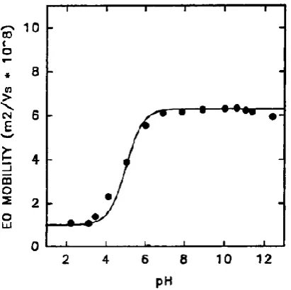
(18) 10. Chapter 2: Electrocavitaton: bottom-up. In case the walls are from glass or quartz, the dissociation of glass surface groups is characterised by the following reaction:. Silicon hydroxide dissociates into silicon oxide ions and protons influence how long and to what extent this process continues. Therefore the surface charge and thereby ζ-potential are dependent on the pH of the solution. In Figure 2.3 the relationship between pH of the solution and the electroosmotic mobility, μEOF, is given from empiric research. From this data the ζpotential can be calculated to be about -85mV at a pH larger than 7.. Figure 2.3: The electroosmotic mobility (μEOF) of glass as a function of pH of the solution. For a pH > 7 this is -8 2 approximately 6⋅ 10 m /Vs. The ζ-potential of this solution is then about -85mV [19].. The thickness of the double layer is typically between 1 and 100 nanometers. For small nanochannels this can pose a problem as double layers from two facing walls can overlap. The typical thickness of the diffuse double layer is also called the Debye length and can be calculated by using the following formula. The number is a result of various constants for aqueous solutions.. √ This is the diffuse double layer thickness in nanometers. I is the ionic strength in Molar or mol per liter. The ionic strength is a measure for the concentration of ions in a solution. It is weighed for the charge number of each ion. For a monovalent saline solution (e.g. NaCl) of 10mM, the Debye length is 3.04nm..

(19) 2.3: A channel with a conductivity step, a rough approach. 2.3. A channel with a conductivity step, a rough approach. In the previous section some of the standards and tools have been described that are used in micro- and nanofluidics. Now it is time to use this knowledge to understand electrocavitation. Consider Figure 2.4. Here a channel is depicted that consists of two solutions: one with a relatively high conductivity and one with a relatively low conductivity. An electrical field is axially applied over the channel. This causes an EOF from the positive to the negative pole as explained in the previous section. However, since a larger part of the electric field will fall over the fluid with the lower conductivity as it has a higher resistance (El>Eh), the resulting EOF velocities will not be equal. The difference in EOF speeds induces a pressure difference and thereby a PDF, to assure equal volume flow in the entire channel. Outside the channel the atmospheric pressure also exerts a force on both ends of the channel, but since they are equal they do not induce a PDF. Now, assuming that volume and charge have to be conserved (it cannot disappear within the channel), the PDF and EOF combined in the low conductivity region must be equal to the PDF and EOF combined in the high conductivity region. In an equation:. Figure 2.4: A channel with two solutions with different conductivities (Kl and Kh). By applying a voltage an EOF with different speed arises in the two solutions. To assure an equal volume flow along the entire channel length, a PDF is generated as indicated. When the front is exactly in the middle, the two PDF flows are equal but in opposite direction. Electric fields and other parameters are indicated.. Two assumptions can be made, simplifying the equations. The first is to assume that the conductivity of one of the solutions is much higher than the other. The EOF velocity in the high conductivity solution can then be neglected. Secondly, when assuming that the front is halfway in the channel, the two PDFs have to balance each other and are therefore equal (but opposite in direction). With these two assumptions it is a simple exercise to calculate the resulting pressure difference at the front when a voltage is applied axially over the channel: and. 11.

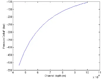
(20) 12. Chapter 2: Electrocavitaton: bottom-up. The resulting pressure is negative in this situation but depends on the polarity of the applied voltage and at which side the high or low conductivity fluid is. The expression for ΔP can function as a crude approximation for the minimum resulting pressure in the system because of the applied electrical voltage (V). It is proportional to the ζ-potential, applied voltage and the permittivity of the solutions and inversely proportional to the height of the channel squared. This has been made visible in Figure 2.5 that plots the channel height versus the resulting pressure with the voltage kept constant at 500V and the ζ-potential assumed to be -50mV. This gives a quick estimation of the possibilities of this technique: for a nanochannel of 45 nanometers high with an applied voltage of 3kV and a ζ-potential of -50mV this pressure can reach up to -311MPa or -3110bar, easily beating the world record set by the quartz inclusions method [20].. Figure 2.5: Possible pressures in bar versus channel depth in nanometers, showing a quadratic relationship. This plot has been generated using the crude approximation for the pressure difference and assuming an applied voltage of 500V and a ζ-potential of -50mV.. 2.4. A channel with a conductivity step, a more exact approach. The previous section provides an easy-to-use and insightful formula for the pressure difference that depends on the channel and solution properties. However, the assumptions made are too crude to expect an accurate representation of reality. Especially the assumption that one of the conductivities is much higher than the other does not hold in practice, where the difference is usually only a few factors instead of orders of magnitude. Keeping the front (X) in the centre is not realistic either. In order to get a more precise result, it is best to start again at the beginning but now fill in the exact formulae..

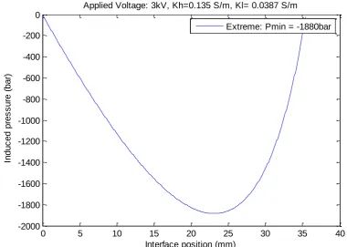
(21) 2.4: A channel with a conductivity step, a more exact approach. (. ) (. 13. ). Now the result is already more precise [20]. In order to solve the equation explicitly, the conduction current through the channel can be calculated by seeing the two different solutions as a series resistance.. Here, Kl and Kh are the conductivities of the low conductive and high conductive solutions, respectively and w is the width of the channel. Now the electrical fields over each part of the channel can be computed.. (. ). (. ). These equations are plugged into the equation for the actual pressure. (. ). ( (. ) ). This is a much more precise formula for the pressure difference. This equation gives the pressure difference for a given channel, its characteristics, the solution characteristics and the position of the front. Plots of this function can now be made to see where the minimum pressure occurs, as done in Figure 2.6 below. What is remarkable, besides the very low pressure reached in this example, is that the minimal pressure is not reached in the middle of the channel. This is because the electric fields over the channel parts are non-linear and non-symmetric. The next step is to calculate this exact position and pressure. For this the derivative of the pressure difference with respect to X should be calculated and equated to zero to find that minimum. (. ). (. √. ). √ (. ).

(22) 14. Chapter 2: Electrocavitaton: bottom-up. Applied Voltage: 3kV, Kh=0.135 S/m, Kl= 0.0387 S/m 0 Extreme: Pmin = -1880bar -200. Induced pressure (bar). -400 -600 -800 -1000 -1200 -1400 -1600 -1800 -2000. 0. 5. 10. 15 20 25 Interface position (mm). 30. 35. 40. Figure 2.6: The pressure difference as a function of the interface position. This has been plotted with a height of 45nm, a length of 35mm, an applied voltage of 3kV, assuming two equal ζ-potentials at -50mV and a ratio of conductivities of about 1:3. The lowest pressure reached in such a setup could be -1880bar or -188MPa.. It is easy to verify that this function is correct by making the assumption again that the difference in conductivity is very high (i.e. a = 0). The equation then reverts back to the first solution for the pressure difference. The formula becomes a little simpler by assuming that the two ζ-potentials are equal. This can only be assumed if the ionic strengths are in the same order of magnitude and the mobility cannot be too different. An experimental optical check can be performed, that is to see if the EOF in one direction (at a certain low voltage) is the same as the EOF in the other direction (at the same but reversed voltage). Another important assumption is that the front between the two conductivities is ‘sharp’. This may not be true since diffusion can make the front more spread out. Every particle in water diffuses a certain distance x over time. √ Where D is the diffusion coefficient of the specific species in water, t the time in seconds and x the distance by the species. The diffusion coefficient of atoms in water is about 2⋅10-9 m2/s, so in one minute species diffuse about 0.5mm. This does not seem very far in a channel of for example 35mm. Moreover, a process called isotachophoresis (ITP) makes sure the front stays sharp when the two solutions have different mobilities. This self-sharpening effect in ITP is due to a difference in mobility of ions. When an electrical field is applied, certain ions will move faster than others. When an ion comes in the zone of the other, it will experience a different field there (either higher or lower) and will move back to its own zone, retaining a sharp boundary..

(23) 2.5: The electrical current and its properties. 2.5. 15. The electrical current and its properties. The electrical (conduction) current measured doing experiments gives plenty information about what is happening in the channel. This has already been briefly mentioned in previous sections. Essentially, the channel can be seen as a series resistor, leading to a formula of the current as described in the previous section. The current can now be used to monitor varies properties of the channel while applying voltages. When an EOF is induced by the application of a voltage over the channel, the current can be seen rising in case the channel gets more and more filled with high conductivity solution. Reversely, it can be seen falling when the channel is more and more filled with low conductivity solution. From this the actual EOF speed can be determined: when the channel is full of either low or high conductivity fluid when the voltage is turned on, an EOF will start filling the channel with the opposite conductivity solution (when the right polarity voltage is applied). During this process the current will rise or lower and eventually stabilise. The time it takes from turning on the voltage to stabilization of the current can be used to calculate the EOF velocity. Since the channel length is known, the velocity is simply the channel length divided by the aforementioned time. The curve of the current between the start and the end situation may or may not be linear, depending on solution concentrations and ζ-potentials [21]. A problem that may arise when voltages are applied for longer time periods (i.e. several minutes) is concentration polarization. Accumulation and depletion at the channel ends cause the current to effectively be lower over time. This process is explained in Figure 2.7. This can be best prevented by flushing the reservoirs around the nanochannel periodically and as often as possible so the solution is always fresh and has the least chance of forming accumulation and depletion zones. Furthermore, applied voltages should be kept low so the currents are not too high.. Figure 2.7: Concentration polarisation. A current is sent from right to left. Inside the nanochannels mainly positive ions conduct the current and in the larger channels, the current is transported by equal amounts of positive and negative ions. At the left-hand exit of the nanochannel therefore more positive ions arrive than are carried away. Since negative ions arrive from the larger channel but cannot enter the nanochannel, also their concentration increases where the microchannel meets the left-hand exit. Both positive and negative ions therefore accumulate on the left-hand side of the nanochannel. On the right-hand side of the nanochannel the reverse process occurs: a depletion zone is formed. Cited from [19]..

(24) 16. Chapter 2: Electrocavitaton: bottom-up. Another important contribution in the electrical current is surface conduction, that is conduction in the diffuse double layer and the Stern layer. Contrary to what is normally assumed, the Stern layer does not seem to be entirely immobile. According to Lyklema et al., the ion mobility of this layer can reach up to 89% of the corresponding bulk value, depending on concentrations and pH, among other things [22]. Conduction in the Stern layer is called anomalous surface conduction. Stein et al. quantify this further, saying the electrical conduction of a nanochannel saturates at a sufficiently low concentration (typically smaller than 10mM), indicating a large role for surface conduction at those low concentrations [23]. This can show up in the electrical current when the channel is drained from fluid and only fluid at the walls and corners of the channel is left. All of this would mean the current would not drop to near zero but retain a specific value. Lastly, we have to consider that the actual electrodes in the solution interact with the fluid. Depending on their material, they can produce H2 or O2 gas when potentials are applied. When the electrodes are small enough, this should pose no problem since the generated quantities of the gasses are so low they will directly dissolve in the solution (though they could then diffuse to other places). Additionally, the interface between electrode and solution also forms a double layer, with its own capacitance, which may take a certain time to charge up when a voltage is applied. However, this can also work the other way around: a small distortion from the system can influence the potential and thereby the current measured at one of the electrode. This would result in measuring errors. Such effects indeed will occur with a polarizable electrode such as a gold electrode and it can be resolved by choosing a non-polarisable electrode such as a silver/silver chloride electrode. Furthermore, inappropriate shielding may cause charges in the solutions to move when a charged object comes nearby. This can be anything from radiation to a human being standing close to the fluid. When charges move, they effectively form an electrical current and therefore interfere with the measurement, which may cause (significant) noise. This is called capacitive charging and can be prevented by shielding of all the fluid by a conductor connected to ground.. 2.6. Putting everything together: electrocavitation. In previous sections the behaviour of a fluid in a channel with a conductivity step is considered. The main result is that a large negative pressure arises when a voltage is correctly applied. Yet a liquid under such a negative pressure is metastable; in time it will change spontaneously to its two-phase system: liquid plus vapour. The pressure will then rise to the equilibrium vapour pressure. The spontaneous formation of vapour in a stressed liquid is called cavitation and this process is also reversible. The investigation into this phenomenon starts at the basic theory of nucleation. At first, homogeneous cavitation in a bulk liquid is considered, meaning heterogeneous cavitation triggered by walls or impurities is not taken into account. The reversible formation of a cavity of a certain volume V requires energy equal to P⋅V where P is the pressure of the liquid. When the liquid is under tension, the energy P⋅V is negative. Formation of a liquid-vapour interface bounding the bubble requires energy equal to σlv⋅A where σlv is the liquid-vapour interface or surface tension and A is the area of the interface. The energy needed to fill the bubble reversibly with vapour of pressure Pv is negative and equal to –Pr⋅V, with V being its volume. The total energy associated with the reversible formation of a spherical vapour bubble with radius r can now be derived [24]..

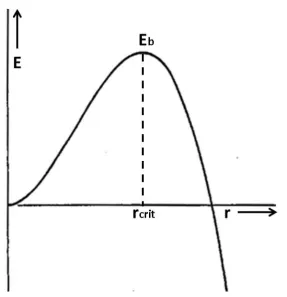
(25) 2.6: Putting everything together: electrocavitation. 17. (. ). In liquids under very high negative pressures, Pr is negligible compared to P and the equation simplifies to:. The energy E is plotted versus r in Figure 2.8 for a negative value of P.. Figure 2.8: The energy of a bubble forming under tension versus its radius. Bubbles with a radius smaller than rcrit will need free energy for further growth; those with a larger radius grow freely. The turning point resembles a barrier. When the pressure gets lower still, both rcrit and Eb will become smaller since they both inversely depend on the pressure. At one point they get so small the liquid becomes metastable and will cavitate at the slightest thermal fluctuation [24].. The curve has a maximum at Eb=16πσlv/3P2 for bubbles with radius rcrit=-2σlv/P. This energy acts as a de facto energy barrier that has to be overcome for the bubble to grow spontaneously. Bubbles with radii less than rcrit require free energy for further growth, while those with radii larger than rcrit grow freely with decreasing free energy. Since bubbles only grow one atom at a time (that is, not all at once), it is evident that bubbles with radii smaller than rcrit will usually disappear without reaching the critical radius [24]. Going back to the nanochannels with a very low pressure, the energy barrier and critical radius will become so low that the liquid in the channel becomes metastable. Any thermal fluctuation can then cause cavitation. When this occurs it can be noticed in two ways. The first is optical, where bubble formation in the channel is visible. The second is by looking at the electrical.

(26) 18. Chapter 2: Electrocavitaton: bottom-up. current. Since the channel can be seen as a series resistor, the highest resistance determines the current. In case of cavitation this means the highest resistance is at the location of cavitation, where the channel contains no more fluid, except the Stern layer at the walls that causes surface conduction. This would show in the value of the current dropping dramatically after a cavitation event. Because this platform is a novel method to generate cavitation, it is dubbed electrocavitation. Note that the cavitation in the nanochannel can also be heterogeneous. This could be caused by surfactant molecules, which reduce the energy cost associated with the creation of a liquidvapour interface or impurities in the solution that change the local structure of the water [9]. In relation to Figure 2.8 this means that that both the energy barrier and critical radius will be lower. Pre-existing bubbles stuck at the surface of the channel can also function as cavitation nuclei. The electrocavitation platform described in the previous sections can also be used to investigate specific species and their behaviour in water. Different species in the solution alter the structure in water, by influencing its bonding and H-bridges. A documented example is the Hofmeister series consisting of saline ions, as shown in Figure 2.9. The hypothesis is that so-called kosmotropes from the left end of the spectrum enhance the H-bond network of water and that chaotropes disorder it. They were originally used to classify the degree of solvability of proteins in a saline solution. It must be noted, however, that this theory is controversial in the scientific community, although it is generally accepted that salts have a disordering effect on the Hbonding network [25]. Electrocavitation may be able to provide further evidence of its validity.. Figure 2.9: Hofmeister series. Combinations of anions and cations on the left are said to enhance the bonding structure of water whereas the ions on the right are said to disrupt it. In electrocavitation this would mean that solutions of kosmotropes would cavitate less quickly than solutions of chaotropes [25]..

(27) Chapter 3: Methodology Before presenting the results the way they are achieved and retrieved has to be made clear. This chapter gives an overview of all the used equipment, devices and solutions. It also presents a framework in which the measurements are performed, including a schematic overview of what happens so outcomes can be better interpreted.. 3.1. The nanochannels and their fabrication. First of all, the nanochannels used in all experiments have to be created. This is done in the cleanroom of the University of Twente. A mask with the channels was designed by Janssen in CleWin [20], as shown in Figure 3.1. It is then used in the cleanroom to create the channels in a 4-inch borofloat glass wafer using lithography. A special photoresistive substance is put on the wafer and spread out. The wafer is then put in a device where it is exposed to light with a specific wavelength through the mask. The photoresistive substance on the part that has been exposed will react and the other part will not. The wafer is then put in a bath to ‘develop’ where all the exposed photoresist will dissolve and disappear. This of course depends on the kind of photoresist and the mask; it could well be the other way around. Finally, the wafer is put in a bath of hydrofluoric acid (HF) for a few minutes to etch away glass only at the parts where the wafer has been exposed to the light (or the other way around in other cases). This creates the channels. The wafer is then cleaned. Along with a dummy wafer it is sent to Leiden University where at the mechanical workshop holes are supersonically drilled in the wafer for the inlets that are connected to the nanochannel. Lastly, the wafers are sent back to the University of Twente where they are subjected to a bonding and annealing step. The exact height of the channel is determined by the use of a Dektak 8 mechanical surface profiler (Veeco Instruments Inc. Plainview, USA). Each wafer contains 19 single channel chips, of which six are 20µm wide, seven are 10µm wide and six are 5µm wide. All channels have rulers and a unique identifier. To obtain the results for this thesis, only the 10μm wide channels are utilised. The height is equal over the whole wafer and varies around 50nm. The length should be 35mm everywhere though because of misalignment of the drilling it may be longer or shorter. This is checked optically through a microscope. The characteristics of all the chips used for this thesis are given in Table 3.1. Table 3.1: The specifics of each wafer and chip used for the experiments.. Wafer number 1 2 2 2. Chip number 10.5 10.2 10.4 10.5. Channel height [nm] 45 53 53 53. 19. Channel length [mm] 35.58 35.45 35.60 35.60.

(28) 20. Chapter 3: Methodology. Figure 3.1: Wafer layout for 19 single channel chips, of which six are 5µm wide, seven are 10µm wide and six are 20µm wide. All have rulers and a unique identifier [20].. 3.2. The setup to perform electrocavitation. To actually measure and influence electrocavitation, the nanochannels have to be placed in a setup where they can be optically monitored, a potential applied, the electrical current measured and new liquids pumped through. The setup is pictured in Figure 3.2. The main apparatus is an Olympus BX51WI microscope with which bright field and fluorescence imaging is performed. The microscope is equipped with a long pass filter cube (488nm excitation, 518nm emission) and a 610 times magnification lens, numerical aperture 0.25 (Olympus Corporation, Tokyo, Japan). Images and movies can be recorded during experiments using a Hamamatsu Orca-ER CCD camera and included HoKaWa software (HAMAMATSU Photonics K.K., Japan) for reference and checking purposes. A custom-built chip interface provides tubing inlets from the top and below, aligned with the chip’s access holes. A more detailed cross section of this interface can be found in Figure 3.3. The table with the platform can be moved to optically check out various sections of the wafer and nanochannels. This is used to determine the precise length of the nanochannel by looking at the exact beginning and end of the channel. It is also used to.

(29) 3.2: The setup to perform electrocavitation. 21. note the exact position of cavitation, if it takes place. The liquids are pumped through the holes of the wafer by the syringe pump shown in the picture; a Standard Infusion Only Pump 22 With Standard Syringe Holder (Harvard Apparatus, USA). This pump can also be controlled through the measurement PC to which the camera is also connected. The voltage source, which is used to apply voltages of up to 3kV over the channel is a HSV488 6000D power supply (LabSmith inc., Livermore, USA) and is controlled by a LabView script. This same script is used to start and stop measurements. Data is gathered by the ground electrode, which is connected to a current-tovoltage (IV) converter and then to a DAC-PCI card at the PC. This IV converter converts the current into a voltage and amplifies it by a factor 108 for the PCI-card. A specific voltage source provides the IV converter circuit with the necessary voltages (+2.5V and -2.5V). The PCI-card has an input range of about -2.2V to +2.2V, which translates to a current between -22nA and 22nA. Digital (pre)processing and analysis of the data is performed using Matlab (MathWorks Inc., Natick, USA). The syringes, tubing and waste containers are extensively shielded and connected to ground.. Figure 3.2: Picture of the setup. The syringes can be seen loaded in the pump below. The wafer with the nanochannels is loaded onto the platform. The microscope and camera can be used to inspect the channels and wafer optically. Figure 3.3 contains a close-up cross section of the platform enclosed by the red rectangle..

(30) 22. Chapter 3: Methodology. Specific enhancements have been made to the setup during this project. First of all, the gold electrodes have been replaced by silver/silver chloride electrodes (see Figure 3.3 and chapter 2.5). This makes the setup more electrochemically stable and thereby also the measured electrical current. Secondly, the syringes were shielded more extensively than before and the outlet tubing and waste container were also shielded. The influence of these modifications on measurement stability was immediately visible. Before, holding an electrically charged item, e.g. a hand, close to the tubing would directly influence the measured current because of charge build-up at the wall of the tubing. Since the electrical current I=dQ/dt, where Q is charge, influencing the charge at a position close to the current measurement electrode directly results in a different current. This is shown schematically in Figure 3.4. Finally, the voltage source turned out to be very noisy so a 50Hz low-pass filter was put directly behind it, greatly reducing the (high frequency) noise from the source, which also showed up in the measured electrical current. This filter introduces a delay in the response in the order of tenths of seconds. However, the events in the cavitation experiments are in the order of seconds so this is considered not to be a problem. During the adjustments made to the setup, certain fluidic leaks started to show up and had to be closed. The overall result is a more electrically and fluidically stable system.. Figure 3.3: Cross section of the platform containing the wafer. The wafer can be aligned such that one chip with one nanochannel can be selected, as is the case on the picture. The drilled holes are then aligned with the teflon tubing through which new liquid can be pumped in the direction indicated by the blue arrows. The liquid can make its way into the nanochannel by either capillary filling or by applying a voltage between the High Voltage (HV) connector (on the right) and ground (on the left), causing an EOF. These two connectors are connected to the power source by a coax-cable. The nanochannels can be optically viewed from above as indicated by the arrow. Elastic O-rings are manually placed into the setup to prevent any leakage. The bottom two are placed first, followed by the wafer and then the top layer with another two O-rings is screwed on top. Silver/silver chloride electrodes have replaced the gold HV and ground electrodes. The ends of the electrode, that actually stick into the solution, are chloridised (picture adapted from [20])..

(31) 3.3: The used solutions and their preparation. 23. Figure 3.4: Holding an electrically charged object (e.g. an electrostatically charged hand) in the vicinity of nonshielded tubing filled with a salty solutions attracts the oppositely charged ions in that solution to the walls of the tubing. This net movement of charge induces an electrical current I n in the solution, which is measured by the current amplifier in superposition with the conduction current I c from the experiments in the nanochannel. This gives a drift on the measured electrical current.. Prior to cavitation experiments, the setup is cleaned with ethanol. The O-rings are kept in a 5050 water/ethanol solution to keep them clean. The whole setup is flushed with deionised water before other liquids are introduced. Channels are optically checked for any defects or particles. After a day of doing experiments, the channels are flushed with water and the wafer is placed in an oven overnight .The oven program consists of 8 hours ramping up to 400°C, 2 hours at 400°C and two hours of ramping down to room temperature. All the channels are now cleared of liquid, improving reproducibility between measurements.. 3.3. The used solutions and their preparation. Now that there is a setup to perform electrocavitation and current measurements, it needs to be provided with solutions to be able to perform electrocavitation. Solutions used are given in Table 3.2. Table 3.2: The solutions used in the experiments. Note that not all these solutions are used for electrocavitation. Some of them are only used to determine the EOF velocity and thereby the ζ-potential in a channel.. Salt used NaHepes NaCl. NaNO3 Na3C3H5O(COO)3(citrate). Concentration [mM] 5 9 10 100 10 100 10 100. Ionic strength [mM] 5 9 10 100 10 100 6 600. Approximate conductivity [mS/cm] 0.39 1.35 1.35 12.29 1.13 11.65 3.03 20.78.

(32) 24. Chapter 3: Methodology. One thing that comes to mind when looking at the used salts is that they all use sodium (Na+) as a counterion. This is chosen deliberately for the whole double layer to consist of Na+-ions only and no other ions so it is more uniform and more likely to have a constant ζ-potential over the whole length of the channel. When the ζ-potential is lower than about -25mV, which is likely, it depends proportionally on the square root of the ionic strength in Molar, that are also given in Table 3.2. Each solution is prepared by solving the necessary amount of salt in 250ml water, taken from a milliQ apparatus. The solutions are then titrated with sodium hydroxide (NaOH) until they reach a pH of 9.5. The reason for this specific pH is that the ζ-potential in a glass nanochannel for this pH value is more negative and stable than for a lower pH (see chapter 2.2 for more details). The solution is constantly monitored by a Hanna HI 4521 pH meter (HANNA instruments Inc. Woonsocket, USA) and stirred during the titration process. The quantities used to get the pH on 9.5 are logged in order to quickly spot irregularities. When the pH of 9.5 is reached, the exact value is noted and the conductivity measured. Sometimes fluorescein is added to the Hepes solution to provide a visual aid for reference and checking purposes. None of the actual cavitation experiments, however, were carried out with fluorescein present. The fluorescein, if used, is always added with a concentration of 0.1mM. After preparation, part of the solution is put in a 30mL vial and degassed using a vacuum pump. A syringe is filled with the solution from the vial so it is then ready to use. A more detailed description of the whole solution preparation and all settings used can be found in Apppendix A. The main reason to not use a buffer to set the pH is that this changes the ions present in the solution and could thereby easily influence the cavitation process, as this directly influences conductivity but also the double layer. A side-effect of not using a buffer, is that the pH is very sensitive to dissolving CO2, which happens constantly when the solution is exposed to air and causes lowering of the pH. CO2 also severely hampers the self-sharpening effect of the front. This also means the solution has to be fresh and quickly used in experiments after it has been prepared. By storing the solution under nitrogen gas this can be partly circumvented, as there should be no CO2 present then to react with the solution. The solution can then still be used after a few days, making experiments a bit more practical. This practice is therefore applied in the experiments carried out for this thesis.. 3.4. Measurements performed using the setup. After describing the channels, setup and used solutions all ingredients are there to perform the electrocavitation measurements. First of all, the setup has to be checked on whether it is functioning correctly. Ideally to achieve this, a specific range of voltages will be applied resulting in a linearly responding electrical current. This is achieved by plugging a resistor into the holes where the fluid normally is. Normal resistors cannot be used since they are not resistant to the high voltages used in the electrocavitation experiments. Therefore special high resistance, high voltage resistors from Hymeg are used (Hymeg Corporation, Addison, USA). They are available in 1GΩ, 10GΩ and 100GΩ. Since the first two give a current above the resolution of the measurement card when voltages above a few hundred Volts are applied, the last one is used. This way, the influence of adjustments and improvements of the setup can be quickly seen by comparing current measurements on the resistor before and after the enhancements. Voltages.

(33) 3.4: Measurements performed using the setup. 25. are applied in a step-wise fashion of about one minute each. The increments between steps are between 100V and 1000V. The polarity is also regularly reversed. To determine the ζ-potential, which is needed to calculate the local negative pressure, the EOF velocity needs to be determined (see chapter 2.2). By applying a relatively low voltage (under 500V), the low conductivity solution will be replaced by the high conductivity solution upon which the electrical current increases or reversely the high conductivity solution will be replaced by the low conductivity solution resulting in a lower current. If the voltage is applied long enough (a few minutes) the entire channel will be filled with one or the other and the current will stabilise. The time this takes can be determined from the electrical current measurements. The EOF velocity is then equal to the channel length divided by this time. The ζ-potential can then be derived directly from the applied field and measured velocity (see equation in chapter 2.2). To check whether the two ζ-potentials in high and low conductivity solution are similar, the polarity can be reversed and the EOF velocity in the other direction can then be measured. The linearity of the current between start and end depends on the conductivity difference as described by Mugele et al. [21]. The species used in these measurements are generally the same as in the cavitation experiments and the measurements are repeated for each channel used. A schematic overview of these measurements is shown in Figure 3.5 part C and D. Marking the Hepes solution with fluorescein can also make it easier to check whether the EOF velocity is constant. The cavitation experiments, then, are performed as shown in Figure 3.5 part C, D and E. First the channel is filled entirely by EOF with low conductivity solution by applying 500V over the channel for 60 or 90 seconds (part C). The voltage is then lowered to 0V for 20 seconds and liquid is pumped through the holes on the side, refreshing the solutions at the entrances of the nanochannel. The pump rate is 30μL/minute for 10 seconds. The voltage is now reversed to 1000V, -2000V or -3000V for 60 seconds. The high conductivity solution will now move into the channel by EOF (part D). The pressure can now become so low that the solution cavitates (part E). Besides optically, this can also be determined electrically since the current will decrease dramatically after a cavitation event. The cavitation time can be taken directly from the current measurements. The position is determined optically as usually one of the solution fronts remains intact and in place, though it has to be verified whether the cavitation position coincides with the front position. This can be done by making a theoretical plot of the front position vs. time, based on the measured ζ-potential, plotting the measured cavitation positions and times into this plot and check whether they coincide with the theoretical position of the front. The voltage is then turned off again for 20 seconds and the channel starts to fill by capillary action while new fluid is pumped through the holes on the sides. The cycle is then repeated by setting the voltage to 500V again for 60 or 90 seconds. Each experiment consists of four cycles..

(34) 26. Chapter 3: Methodology. Figure 3.5: Schematic overview of electrocavitation experiments. A) the channel starts empty. B) low conductivity (green) fluid is introduced at well B and starts to fill the nanochannel by capillary action. C) both wells are flushed at 0V with fresh solution to remove contamination (bubbles from filling or from previous experiments and concentration polarization). Next, 500V is applied for 60 or 90 seconds, to ensure the whole channel is filled with low conductivity solution and that bubbles are removed. D) both wells are flushed again at 0V. This time -1000V, 2000V or -3000V is applied for 60 seconds. High conductivity solution (blue) starts replacing the low conductivity solution by EOF. E) cavitation may take place. If it does, the position is determined optically and the time from the electrical current measurements. The cycle then starts at C) again. Each experiment consists of four cycles.. The solutions used in cavitation experiments are NaHepes 5mM (low conductivity) and NaCl 10mM (high conductivity), NaCl 10mM and 100mM, NaNO3 10mM and 100mM and Na3C3H5O(COO)3 10mM and 100mM. When a cavitation event occurs, the view from the microscope is as in Figure 3.6.. Figure 3.6: A cavitation event. In this case the low conductivity fluid is drained to the right. The difference between the two shots is one frame of 0.2s. The front remains intact at 13.72mm. The front may not be the same as the cavitation position; this has to be verified by checking the theoretical position of the front vs. the cavitation position and time..

(35) Chapter 4: Experimental results This chapter delivers and discusses results based on the theory and methodology of the previous chapters. The improvements made to the setup are examined, EOF measurements are performed to determine the ζ-potential and electrocavitation measurements are presented and discussed in relation to the achieved minimum pressure. Finally, an investigation into using salts from the Hofmeister series is carried out.. 4.1. Current measurements before and after improvements. First of all the results of the improvements to the setup made during this project are presented. Step-wise increments of the voltage have been applied over a 100GΩ resistor. The results are shown in Figure 4.1. The measurements before adjustments are on the left, those after adjustments on the right. The reduction of the noise is the most obvious difference, especially at negative voltages. This gives the measured current a higher accuracy. The peaks in the signal have also disappeared. It must however be noted that the signal still contains some noise, specifically at negative voltages. The improvement is most likely caused by the 50Hz filter, which blocks a lot of noise coming from the power source. The additional shielding and change of electrode material will not have much of an effect on these kind of measurements, since no fluids are involved. The effect of the 50Hz filter can be found back in the current response, which takes longer to reach its maximum.. Figure 4.1: Electrical current measurements performed on a 100GΩ resistor before (on the left) and after (on the right) improvements of the setup were made. The noise after the improvements is significantly less than before; there is however still some noise at negative voltages.. Additionally, electrocavitation experiments are performed before and after the adjustments, leading to a drastic change, see Figure 4.2. Again, the noise decreases drastically. Moreover, whereas the left signal is almost useless in determining the exact cavitation time due to the erratic drift obscuring other signals (see section 4.3), the right picture is clearer and more stable. This is most likely due to the replacement of the electrodes by non-polarisable electrodes and the additional shielding, which takes all the random frequency drift out of the signal. This is a. 27.

(36) 28. Chapter 4: Experimental results. significant achievement as it greatly enhances the results because the cavitation time can now be determined much more precisely.. Figure 4.2: Electrocavitation experiments of four cycles performed before (on the left) and after (on the right) improvements to the setup were made. Note the reduction of noise and the lack of a random drifting current.. 4.2. EOF measurements to determine the ζ-potential. Now that it is verified that the setup produces reliable electrical current measurements, actual measurements on electrocavitation can start. Before that, though, the ζ-potential for each used channel has to be determined in order to interpret electrocavitation measurements and calculate the minimum pressure. This is done for every channel used for electrocavitation experiments, immediately prior to experiments. The ζ-potential is assumed to be constant in the whole channel. As described in chapter 3, these measurements are performed by applying a low enough voltage (usually 200V or -200V) so the solution does not cavitate and the high conductivity solution is replaced by the low conductivity solution or vice versa. An example is shown in Figure 4.3. Here, the higher conductivity NaCl 10mM solution is replaced by the lower conductivity 9mM NaCl solution. The current stabilises when the replacement of one by the other is completed, in this case the replacement of 10mM solution by 9mM solution. The exact length of the channel divided by the time this takes is then the EOF velocity. The ζ-potential can be derived directly from this velocity using the formula for EOF velocity from section 2.2. The main disadvantage of using these lower voltages is that the signal becomes more susceptible to noise, also visible in this example. This makes it harder to determine the exact time and thereby the ζ-potential which can then no longer be determined precisely. EOF-measurements with NaCl 10mM and Hepes 5mM solution are also conducted. However, in those measurements it is usually less clear when the current stabilises at the lower or higher level, making it even harder to determine the replacement time and related ζ-potential. Still, values for the replacement time were found to be similar with those found in the other experiments (where 10mM NaCl is replaced by 9mM NaCl). The value of the ζ-potential was found to be around -60mV with values up to -65mV and down to -55mV. This is lower than expected since for solutions of about 10mM at pH 9.5, a ζ-potential of about -85mV is predicted by theory (see section 2.2)..

No results found